Critical Assessment of Wave-Particle Complementarity
via Derivation from Quantum Mechanics

Fedor Herbut

Abstract After introducing sketchily Bohr’s wave-particle complementarity principle in his own words, a derivation of an extended form of the principle from standard quantum mechanics is performed. Reality-content evaluation of each step is given. The derived theory is applied to simple examples and the extended entities are illustrated in a thought experiment. Assessment of the approach of Bohr and of this article is taken up again with a rather negative conclusion as far as reflecting reality is concerned. The paper ends with quotations of selected incisive opinions on Bohr’s dogmatic attitude and with some comments by the present author.

Keywords Copenhagen interpretation, quantum-mechanical insight in experiments, search of quantum-mechanical reality

1 Introduction

Recent investigation [1], [2], [3], has shown that the relative-reality-of-wave-function point of view gives good insight in some intricate experi-

 

F. Herbut (mail)
Serbian Academy of Sciences and Arts, Knez Mihajlova 35, 11000 Belgrade, Serbia
e-mail: fedorh@infosky.net and from USA etc. fedorh@mi.sanu.ac.yu

ments. This may come as a surprise in view of the well-known fact that for a very long time Bohr and Copenhagen reigned the field. One of the leading ideas was Bohr’s wave-particle complementarity (or duality) principle. This investigation is aimed at a critical derivation of it, or rather of its natural extension, from quantum mechanics, and at an appraisal from the point of view of the reality-of-state approach. A precise criterion will emerge distinguishing Bohr’s case from the extension.

To begin with, one should remember the often quoted commentary of Einstein [4]:

Quote EINSTEIN: ”… Bohr’s principle of complementarity, the sharp formulation of which, moreover, I have been unable to achieve despite much effort which I have expended on it.” (Emphasis by F. H.)

Complementarity, in contrast to indeterminacy, seems to have remained unsettled between Einstein and Bohr.

There were other disquieting events concerning complementarity. As early as in 1951 a no lesser physicist than Max Born expressed doubts in one of his books [5]:

Quote BORN: ”The conceptions ”particles” and ”waves” have no such complementary character (he means Bohr’s ’mutual exclusion’ of the corresponding experiments, F. H.), as in many cases both are needed …”

Further, there is the paradox (with respect to Bohr’s wave-particle complementarity principle) of Ghose and Home [6] in a real experiment. This important work, and some other thought experiments [7], [8] indicate that Bohr’s intuitive complementarity principle was too narrowly conceived. It may be that in Bohr’s time one did not think of sophisticated experiments; the simple ones seemed quite baffling.

It is well known that the formal structure of quantum mechanics has had unparalleled success in predicting probabilities of measurement results in microscopic phenomena. Not one prediction of the former was proved false in the latter.

In an attempt to derive a sharp form of wave-particle duality, we will deal with experiments in which an observable with a purely discrete spectrum is exactly measured. In other words, experiments with positive-operator-valued measures (POVM) and inexact (or unsharp) measurements are outside the scope of this study.

We start by a glance at Bohr’s idea of the duality in question.

2 On Bohr’s Wave-Particle Complementarity Principle

I’ll present what I think is the most important part of Bohr’s complementarity principle in four quotes of Bohr’s own words. In the first [9], Bohr explains what the problem is in the example of the well-known Mach-Zehnder interferometer [10] (cf the upper part of the Figure in subsection 9.1).

Quote BOHR1: ”The extent to which renunciation of the visualization of atomic phenomena is imposed upon us by the impossibility of their subdivision is strikingly illustrated by the following example to which Einstein very early called attention and often has reverted. If a semi-reflecting mirror is placed in the way of a photon, having two possibilities for its direction of propagation, the photon may either be recorded on one, and only one, of two photographic plates situated at great distances in the two directions in question, or else we may, by replacing the plates by mirrors, observe effects exhibiting an interference between the two reflected wave-trains. In any attempt at a pictorial representation of the behavior of the photon we would, thus, meet with the difficulty: to be obliged to say on the one hand, that the photon always chooses one of the two ways and, on the other hand, that it behaves as if it had passed both ways.” (Emphasis by F. H.)

In the next quote [11] Bohr expounds his answer to the ”difficulty”, in terms of his famous principle of complementarity:

Quote BOHR2: ”Information regarding the behavior of an atomic object obtained under definite experimental conditions may, however, according to a terminology often used in atomic physics, be adequately characterized as complementary to any information about the same object obtained by some other experimental arrangement excluding the fulfillment of the first conditions. Although such kinds of information cannot be combined into a single picture by means of ordinary concepts (i. e., by assuming that the descriptive terms in the complementary descriptions refer to ”the same object”), they represent indeed equally essential aspects of any knowledge on the object in question which can be obtained from this domain.” (Emphasis by F. H.)

Another quote [12] sums up complementarity in a less bulky way:

Quote BOHR3: ”…evidence obtained under different experimental conditions cannot be comprehended within a single picture, but must be regarded as complementary in the sense that only the totality of the phenomena exhausts the possible information about the objects.”

In application to the Mach-Zehnder ’difficulty’ (see Quote BOHR1), the complementarity principle treats the which-path and the interference versions (described in Quote BOHR1) as two complementary experiments. Hence, the ’visualizations’ or ’pictorial representations’ in them cannot be combined. In such a manner Bohr solves the mentioned mind-boggling perplexity. This is so even in Wheeler’s well-known delayed-choice version [13], in which the choice between ’which-path’ or ’interference’ is made after the photon has passed the semi-reflecting mirror. This is clear from the immediate continuation of quote BOHR1:

Quote BOHR4: ”It is just arguments of this kind which recall the impossibility of subdividing quantum phenomena and reveal the ambiguity in ascribing customary physical attributes to atomic objects.” (Emphasis by F. H.)

In my understanding, by ’subdivisions’ (cf also quote BOHR1) Bohr means both spatial and temporal ones.

3 Introduction into Visualization Theory

As well known, Bohr applied classical physics to the behavior of the macroscopic measuring agency that measures some observable  $A\enspace$ at the final moment  $t_{f}\enspace$ of some experiment. But he did more than that. He pushed description in terms of classical physics also into an answer to the question ’What happens in the experiment?’. As we saw in Quotes BOHR2 and BOHR3, he called this ’visualization’ or ’pictorial representation’. One wonders why he did go so far with classical description. Perhaps, we can find an answer in the following quote [14].

Quote BOHR5: ”The language of Newton and Maxwell will remain the language of physicists for all time” (Emphasis by F. H.)

For a thorough discussion of this point see Schlosshauer [15].

Reichenbach has pointed out that three-valued logic is more in the spirit of quantum mechanics than the standard two-valued one [16]. But we do think in terms of two-valued logic. Perhaps for this reason, three-valued logic did not find much application in quantum mechanics or its philosophy. It seems to me that Bohr believed that the situation is similar with physics. According to him, apparently, we cannot help viewing the world around us in terms of classical physics. This is one of the reasons, perhaps why Bohr strived to pervade quantum mechanics with classical physics as much as possible.

Some prerequisites for a theory are now going to be presented. They are meant to be the basis of a derived sharp form of the complementarity principle.

Let us consider a quantum experiment. It begins, at an initial moment  $t_{i},\enspace$ with a prepared spatial ensemble of quantum systems, or with a single individual system from the, experimentally and theoretically identical, time ensemble. Both the ensemble and each individual system in it are described by some density operator  $\rho(t_{i})\enspace$ (mostly by the special case of a state vector or wave function - as often said). The elements of the ensemble are assumed to be non-interacting with each other and with the environment. Thus, due to dynamical isolation, one has evolution with a unitary operator  $U(t_{f}-t_{i},t_{i})\enspace$ in the Schrödinger picture. Throughout this paper, we shall omit the moment when the operator is applied. It will be understood that it is at the earlier of the two moments defining the time interval of evolution. Thus,

$$\rho(t_{f})=U(t_{f}-t_{i})\rho(t_{i})U(t_{f}-t_{i})^{{\dagger}},$$

where the dagger denotes adjoining (and, in this case, adjoint equals inverse).

As it has been stated, it is assumed that we have exact measurement of an ordinary, complete or incomplete, observable with a purely discrete spectrum at the final moment  $t_{f}\enspace$. Let  $A\enspace$ be the Hermitian operator representing it in the formalism, and let its spectral form be

$$A=\sum_{n}a_{n}P_{n},\quad n\not=n^{\prime}\enskip\Rightarrow\enskip a_{n}\not=a_{n^{\prime}}.$$

(The index or quantum number  $n\enspace$ enumerates the distinct eigenvalues  $a_{n}\enspace$ and eigen-projectors  $P_{n}.\enspace$ ) The accompanying spectral decomposition of the identity is

$$\sum_{n}P_{n}=I,$$

where  $I\enspace$ denotes the identity operator. Relation (2b) is also called the relation of completeness and also the closure property. The sum in (2b) has at most a countable infinity of orthogonal projector terms.

In many experiments, the completeness relation (2b) makes the spectral form (2a) superfluous, i. e., one talks in terms of eigen-events  $P_{n}\enspace$ without eigenvalues  $a_{n}$.

As it is well known, the measuring apparatus detects a result  $a_{n}\enspace$ (cf (2a)) or, more generally put, the occurrence of an eigen-event  $P_{n}\enspace$, in the state  $\rho(t_{f})\enspace$ for each individual system. As to the ensemble, the observed relative frequency of the result is close to the predicted probability value, given by the so-called trace formula (the up-to-date equivalent of Born’s rule)

$$p_{n}={\rm tr}\Big{(}P_{n}\rho(t_{f})\Big{)}.$$

(One should obtain equality in the limes of an imagined infinitely large ensemble.)

We give now a formal definition of the retrospective observables  $A^{r}(t)\enspace$,  $t_{i}\leq t<t_{f}\enspace$, the Hermitian-operator representatives of which have the spectral forms:

$$A^{r}(t)\equiv\sum_{n}a_{n}P_{n}^{r}(t),\quad n\not=n^{\prime}\enskip\Rightarrow\enskip a_{n}\not=a_{n^{\prime}},$$

with the definition of retrospectivity at the moment  $t\enspace$:

$$\forall n:\quad P_{n}^{r}(t)\equiv U^{{\dagger}}(t_{f}-t)P_{n}U(t_{f}-t).$$

(It may be sometimes suitable to allow the eigenvalues of  $A^{r}(t),\enspace$ if they have a physical meaning, not to be necessarily equal to those of  $A\enspace$ because it is the projectors that count.) Naturally, (2b) implies the completeness relation

$$\sum_{n}P_{n}^{r}(t)=I.$$

Besides the actually measured observable  $A\enspace$ and its formal images  $A^{r}(t)\enspace$, which are ’back-evolved’ to a moment  $t\enspace$, let also new observables  $B(t)\enspace$, ’jokers’ for the time being, be introduced. They will play a natural role in completing the forthcoming derivation.

Let also the observables  $B(t)\enspace$ be defined in spectral form

$$B(t)=\sum_{k}b_{k}Q_{k}(t),\quad k\not=k^{\prime}\enskip\Rightarrow\enskip b_{k}\not=b_{k^{\prime}},$$

with the completeness relation

$$\sum_{k}Q_{k}(t)=I$$

for the eigen-projectors. We consider  $B(t)\enspace$ as given at the initial or some intermediate moment  $t$.

It will also be useful to formally evolve  $B\enspace$ to the final moment  $t_{f}\enspace$ when the actual measurement of  $A\enspace$ takes place. One has

$$B^{f}\equiv U(t_{f}-t)B(t)U(t_{f}-t)^{{\dagger}},$$

$$\forall k:\quad Q_{k}^{f}=U(t_{f}-t)Q_{k}(t)U(t_{f}-t)^{{\dagger}}$$

(cf the convention adopted above (1)).

One should remember that it is the Schrödinger picture that is being made use of. The evolution (or ’back evolution’) of an observable are auxiliary concepts (nothing to do with the Heisenberg dynamical picture).

4 Blindness to Coherence in Measurement

Let us return to the actually measured observable  $A\enspace$ in the final state  $\rho(t_{f})\enspace$, and let us define the coherence-deprived mixture

$$\rho(t_{f})_{M}\equiv\sum_{n}p_{n}\rho(t_{f})_{M}^{n}$$

corresponding to  $A\enspace$, where the (statistical) weights are the probabilities  $p_{n}\enspace$ given by (3), and

$$\forall n,p_{n}>0:\quad\rho(t_{f})_{M}^{n}\equiv P_{n}\rho(t_{f})P_{n}\Big{/}p_{n}$$

are the constituent states of which the mixture consists (concerning  $n\enspace$, cf (2a)). One should note that if  $p_{n}=0,\enspace$ then, as it is usually understood, the entire corresponding term in (7a) is zero - in spite of the fact that the corresponding density operator (7b) is not defined. (This will not be mentioned again for other formal mixtures below.)

In each state defined by (7b) the observable  $A\enspace$ has the definite corresponding value  $a_{n}\enspace$. This is so because  ${\rm tr}\Big{(}P_{n}\rho(t_{f})_{M}^{n}\Big{)}={\rm tr}\Big{(}\rho(t_{f})_{M}^{n}\Big{)}=1\enspace$.

It is possible coherence that makes a difference between a given state  $\rho(t_{f})\enspace$ and the corresponding mixture (7a). It is important to be aware that ’coherence’ is a relative concept that applies to a state in relation to an observable (for more details see [17]). In this case we have possible coherence in  $\rho(t_{f})\enspace$ in relation to  $A\enspace$.

In view of the fact that one can always write  $\rho=\sum_{k}\sum_{k^{\prime}}Q_{k}\rho Q_{k^{\prime}}\enspace$ (cf the completeness relation (5b)), one can, in general, define coherence as follows.

Definition 1. A state  $\rho\enspace$ is coherent with respect to an observable  $B\enspace$ if  $\sum_{k\not=k^{\prime}}Q_{k}\rho Q_{k^{\prime}}\not=0\enspace$ (cf (5a)), or, equivalently, if  $\exists k\not=k^{\prime}:\enskip Q_{k}\rho Q_{k^{\prime}}\not=0$.

In (7a) the state is by ’brute force’ deprived of all possible coherence among the distinct values of  $A\enspace$ in  $\rho(t_{f})=\sum_{n,n^{\prime}}P_{n}\rho(t_{f})P_{n^{\prime}}\enspace$. (As to a measure for the amount of coherence, see [17].) This is why Bell calls (7a) the ’butchered’ version of  $\rho(t_{f})\enspace$ [18].

It is a crucial fact that, in spite of the ’butchering’, one obtains the same individual-system results and the same relative frequencies when  $A\enspace$ is measured in  $\rho(t_{f})\enspace$ or in  $\rho(t_{f})_{M}\enspace$ (cf (7a)). Thus, the measuring apparatus cannot distinguish the final state  $\rho(t_{f})\enspace$ from the corresponding ’butchered’ mixture (7a) in the given experiment , i. e., it is blind to the possible coherence in  $\rho(t_{f})$.

Next, let us define the mixture corresponding to the initial or intermediate state  $\rho(t)\equiv U(t-t_{i})\rho(t_{i})U(t-t_{i})^{{\dagger}}\enspace$,  $t_{i}\leq t<t_{f}\enspace$, and the corresponding retrospective observable  $A^{r}(t)\enspace$ (cf (4a) and (4b)). But first let us establish (by inserting the evolution operator) that the initial or intermediate and the final probabilities are equal:

$$\forall n:\quad{\rm tr}\Big{(}P_{n}^{r}(t)\rho(t)\Big{)}={\rm tr}\Big{[}\Big{(}U(t_{f}-t)^{{\dagger}}P_{n}U(t_{f}-t)\Big{)}\Big{(}U(t_{f}-t)^{{\dagger}}\rho(t_{f})U(t_{f}-t)\Big{)}\Big{]}=$$

$${\rm tr}\Big{(}P_{n}\rho(t_{f})\Big{)}=p_{n}$$

(cf (1), (3) and (6a)).

The ’butchered’ mixture that we want to write down is:

$$\rho(t)_{M}\equiv\sum_{n}p_{n}\rho(t)_{M}^{n},$$

where

$$\forall n,p_{n}>0:\quad\rho(t)_{M}^{n}\equiv P_{n}^{r}(t)\rho(t)P_{n}^{r}(t)\Big{/}p_{n}$$

(cf (4b)).

The unitary evolution by  $U(t_{f}-t)\enspace$ takes the initial or intermediate mixture (8a) into the final mixture (7a). Therefore, in the given experiment the state  $\rho(t)\enspace$ and the corresponding ’butchered’ mixture  $\rho(t)_{M}\enspace$ in relation to  $A^{r}(t),\enspace$ cannot be distinguished neither on the individual-system level, nor as ensembles.

5 The ’Simplest Which-Result’ Visualization Theory

The retrospective observable  $A^{r}(t)\enspace$ (cf (4a)) is, in general, just a mathematical construction. But in some experiments it has a physical meaning. Then we have the ’simplest which-result’ visualization. It is slightly more general than the case of Bohr’s particle-like visualization (see below).

The visualization at issue consists of two drastic imagined steps of changes.

(i) Whereas the true initial or intermediate state  $\rho(t),\enspace$ which, in general, contains coherence in relation to  $A^{r}(t)\enspace$, describes both a laboratory ensemble and each individual system in it, in the visualization it is the ’butchered’ mixture  $\rho(t)_{M}\enspace$ (cf (8a)) without the possible coherence that describes the ensemble.

(ii) Resorting to the so-called ’ignorance-interpretation’ of a mixture used in classical physics, the individual system is described by one of the constituent states  $\rho(t)_{M}^{n}\enspace$ in the mixture (cf (8b)).

In visualization, the ensemble state  $\rho(t)_{M}\enspace$, given by (8a), is a mixture of the individual-system states states given by (8b).

It is important to keep in mind that the state (8b) has the definite property  $a_{n}\enspace$ of the retrospective observable  $A^{r}(t)\enspace$ (cf (4a-c)), or, equivalently, that the eigen-event  $P_{n}^{r}(t)\enspace$ of  $A^{r}(t)\enspace$ occurs in it.

The ’simplest which-result’ visualization, which is being expounded, is based on the following relations, which are easily seen to follow from the definitions (4a) and (4b):

$$A^{r}(t)\equiv U(t-t_{i})A^{r}(t_{i})U(t-t_{i})^{{\dagger}}=\sum_{n}a_{n}U(t-t_{i})P_{n}^{r}(t_{i})U(t-t_{i})^{{\dagger}}=\sum_{n}a_{n}P^{r}(t)$$

(cf (4a) and (4b)), and

$$\forall n,\enskip p_{n}>0:\quad\rho(t)_{M}^{n}=U(t-t_{i})\rho(t_{i})_{M}^{n}U(t-t_{i})^{{\dagger}}=$$

$$U(t-t_{i})\Big{(}P_{n}^{r}(t_{i})\rho(t_{i})P_{n}^{r}(t_{i})\Big{/}p_{n}\Big{)}U(t-t_{i})^{{\dagger}}=$$

$$\Big{(}U(t-t_{i})P_{n}^{r}(t_{i})U(t-t_{i})^{{\dagger}}\Big{)}\Big{(}U(t-t_{i})\rho(t_{i})U(t-t_{i})^{{\dagger}}\Big{/}p_{n}\Big{)}\Big{(}U(t-t_{i})P_{n}^{r}(t_{i})U(t-t_{i})^{{\dagger}}\Big{)}=$$

$$P_{n}^{r}(t)\rho(t)P_{n}^{r}(t)\Big{/}p_{n},$$

where  $t_{i}\leq t\leq t_{f}\enspace$, and  $A^{r}(t_{f})=A\enspace$. Thus, the individual system is at each instant  $t\enspace$ imagined to be in a state  $\rho(t)_{M}^{n}\enspace$, which has the definite value  $a_{n}\enspace$ of  $A^{r}(t)\enspace$.

In most cases  $A\enspace$ and all its ’back-evolved’ forms  $A^{r}(t)\enspace$ are localization observables. Then, one speaks of ’which way’ instead of ’which result’, and one imagines that the system behaves as a particle moving along a trajectory (particle-like behavior). If, in addition, the initial observable  $A^{r}(t_{i})\enspace$ has the physical meaning of localization, i. e., if the quantum-mechanical ’trajectory’ begins at the initial moment, then one has Bohr’s particle-like behavior in the famous wave-particle duality relevant for a large number of experiments.

6 A More Practical Criterion

Remark 1 It is easy to see that in the ’simplest which-result’ case that we consider,  $A^{r}(t_{i})\enspace$ satisfies the assumptions of premeasurement ([19] and [20]):  $A^{r}(t_{i})\enspace$ appears to be the measured observable,  $A\enspace$ the ’pointer observable’, and the macroscopic (classically described) measuring agency appears to play the role of objectification (or ’reading’ the result).

It is not always easy to evaluate the action of the formal back-evolving operator  $U(t_{f}-t)^{{\dagger}}\enspace$ on the measured observable  $A\enspace$. Hence a more practical criterion is desirable.

We resort to the ’joker’ observable  $B\enspace$ (cf (5a)), and make use of it having in mind that ’simplest which-result’ visualization consists in the fact that there exists an observable  $B\enspace$ with physical meaning and the equality  $B=A^{r}(t)\enspace$ holds true.

Theorem 1 A necessary and sufficient condition for a ’which-result’ visualization: If an observable  $B(t)\enspace$,  $t_{i}\leq t<t_{f}\enspace$, has physical meaning and, having in mind the quantum numbers of  $B(t)\enspace$ and  $A\enspace$ (cf (5a) and (2a) respectively), there exists a bijection (a one-to-one ’onto’ map)  $k\rightarrow n=n(k)\enspace$ such that for each value of the index  $k,\enspace$ whenever a state  $\rho(t)\enspace$ has the property  $b_{k},\enspace$ or, equivalently, the event  $Q_{k}\enspace$ occurs in  $\rho(t),\enspace$ then the final state  $\rho(t_{f})\enspace$ gives the result  $a_{n(k)}\enspace$ in the measurement of  $A\enspace$ with certainty, i. e.,

$${\rm tr}\Big{(}\rho(t)Q_{k}(t)\Big{)}=1\quad\Rightarrow\quad{\rm tr}\Big{(}\rho(t_{f})P_{n(k)}\Big{)}=1.$$

If the condition is valid, then  $B(t)=A^{r}(t)\enspace$, and one has ’which-result’ visualization.

Proof is given in Appendix A.

Remark 2 Theorem 1 implies that the retrospective observable  $A^{r}(t)\enspace$, and no other observable (up to the eigenvalues  $a_{n}\enspace$, which are irrelevant), has the required property. The property itself can be experimentally demonstrated (see the examples below) by showing that any initial state with any definite value  $b_{k}\enspace$ of a given observable  $B\enspace$ with a physical meaning necessarily ends up in a state with the definite value  $a_{n(k)}\enspace$ of the actually measured observable  $A.\enspace$ If the ’which-result’ experiment is understood as measurement of  $A^{r}(t_{i})\enspace$ via the ’pointer observable’  $A\enspace$ (cf Remark 1), then the theorem says that the latter measures precisely one observable (up to arbitrary eigenvalues).

Incidentally, I have discussed backward ’projection’ in time of an actually measured observable in two previous articles in contexts different from the present one [20], [21].

7 Completion of the ’Interference’ or ’Which-Result’ Visualization

Remark 3 To develop a full visualization theory, one needs to answer two questions:

(i) Can one have a ’which-result’ experiment without one of the retrospective observables  $A^{r}(t)\enspace$ being physically meaningful?

(ii) If one does not have a ’which-result’ experiment, does one ipso facto have a wave-like or ’interference’ pictorial representation?

To answer the two questions in Remark 3, we turn to the other alternative in Bohr’s wave-particle complementarity principle: to the wave.

Classical waves are essentially different from quantum-mechanical wave-like behavior, which is universal and contained in the very time evolution (1) of any quantum-mechanical state  $\rho(t_{i}).\enspace$ Let us take as a simple example diffraction of a photon through one hole. (This case puzzled Einstein in Solvey 1927 [22].)

On passing the hole, the evolution of the photon can be understood in a simplified, coarse-grained way as consisting of a diverging coherent bundle of component probability amplitudes constituting a half-sphere. When the photon is located, one of the components is realized, and all the others just disappear, become mysteriously extinguished. (This is the collapse version of quantum-mechanical insight.)

Locating a photon in a dot out of a half-sphere is only quantitatively (not qualitatively) different from the case of the Mach-Zehnder which-way device. (In the latter only one component is extinguished.)

Returning to classical wave-like behavior, here we have components that are real in the classical sense. Their reality is detectable: all components simultaneously influence the result of measurement (or measurements). This idea leads us to the basic Definition 3 below, which distinguishes ’which-result’ experiments from ’interference’ ones.

Coherence (see Definition 1) is usually detected as interference. Let  $B\enspace$ (cf (5a)) be an observable that has physical meaning at some moment  $t,\enskip t_{i}\leq t\leq t_{f}\enspace$ in the experiment.

Definition 2 A state  $\rho(t)\enspace$ exhibits interference in relation to an observable  $B\enspace$ in the measurement of an observable  $A\enspace$ (cf (2a)) if for at least one eigenvalue  $a_{n}\enspace$ of  $A\enspace$ the state  $\rho(t)\enspace$ predicts a different probability than the ’butchered’ mixture corresponding to  $B\enspace$:

$$\rho(t)_{M,B}\equiv\sum_{k}p_{k}\rho(t)_{M,B}^{k}\enskip,$$

where the statistical weights are

$$\forall k:\quad p_{k}\equiv{\rm tr}(Q_{k}\rho(t))$$

(cf (5a)), and the definite-result states of  $B\enspace$ are

$$\forall k,p_{k}>0:\quad\rho(t)_{M,B}^{k}\equiv Q_{k}\rho(t)Q_{k}\Big{/}p_{k}.$$

In Definition 2 ”predicts” is short for ”the corresponding time-evolved state  $\rho(t_{f})\enspace$ predicts”. Thus, on the one hand we have  ${\rm tr}\Big{(}\rho(t_{f})P_{n}\Big{)}\enspace$ (cf (2a)) with  $\rho(t_{f})=U(t_{f}-t))\rho(t)U(t_{f}-t))^{{\dagger}}\enspace$. On the other hand, we have  ${\rm tr}\Big{[}\Big{(}U(t_{f}-t))\rho(t)_{M,B}U(t_{f}-t))^{{\dagger}}\Big{)}P_{n}\Big{]}\enspace$. Interference has set in if these two probabilities differ for at least one value of  $n$.

Definition 3 A) We say that an observable  $B\enspace$ (cf (5a)) with a physical meaning at some moment  $t,\enskip t_{i}\leq t\leq t_{f}\enspace$, is a ’which-result’ observable in the given experiment that ends in the measurement of  $A,\enspace$ and the experiment is a ’which-result’ one in relation to  $B\enspace$, if the final state  $\rho(t_{f})\enspace$ exhibits no interference in comparison with the corresponding mixture  $U(t_{f}-t)\rho(t)_{M,B}U(t_{f}-t)^{{\dagger}}\enspace$ (cf Definition 2)).

B) We say that an observable  $B\enspace$ with a physical meaning at a moment  $t\enspace$ is an ’interference’ one, and the experiment is an ’interference’ one in relation to  $B\enspace$ if there exists at least one physically meaningful initial state  $\rho(t_{i})\enspace$ that shows interference with respect to  $B\enspace$ in the measurement of  $A\enspace$. (Needless to say that this  $\rho(t_{i})\enspace$ then must a fortiori contain coherence with respect to  $B\enspace$.)

The first question in Remark 3 is now going to be answered by deriving a necessary and sufficient condition for ’which-result’ visualization. The condition will simultaneously answer also the second question in the affirmative.

Theorem 2 ’Interference’ or ’which-result’ visualization Let  $B(t)\enspace$ be a physically meaningful observable at some moment  $t,\enskip t_{i}\leq t<t_{f}\enspace$ in the given experiment.

A) The observable  $B(t)\enspace$ is a ’which-result’ one and the experiment is of the same kind in relation to  $B\enspace$ if and only if its evolved form  $B^{f}\equiv B(t_{f})\enspace$ (cf (6a)) and  $A\enspace$ are compatible, i. e., they commute as operators

$$\Big{[}B^{f},A\Big{]}=0.$$

In more detail, any initial state  $\rho(t_{i})\enspace$ and the corresponding ’butchered’ state  $\rho(t_{i})_{M,B}\enspace$ (cf (11a-c)) predict the same probability for every value  $a_{n}\enspace$ of the actually measured observable  $A\enspace$ if and only if (12) is valid.

B) If  $B(t)\enspace$ is not a ’which-result’ observable, then ipso facto  $B(t)\enspace$ and the experiment in relation to it are ’interference’ ones. More precisely, in this case there exists, in principle, a physically meaningful initial state  $\rho(t_{i})\enspace$ such that it ’predicts’ at least for one result  $P_{n}\enspace$ of  $A\enspace$ a different probability than the corresponding ’butchered’ mixture  $\rho(t)_{M,B}\enspace$ .

Proof is given in Appendix B.

Remark 4 One should note the relative character of a ’which-result’ or ’interference’ experiment. But one can say, in the spirit of Bohr’s wave-particle complementarity principle, if there exists at least one physically meaningful observable  $B\enspace$ at some instant  $t\enspace$,  $t_{i}\leq t\leq t_{f}\enspace$ in relation to which the experiment is a ’which-result one’, then the experiment can be viewed as such in an absolute sense.

Remark 5 A physically meaningful observable  $B\enspace$ that is not the back-evolved measured observable  $A\enspace$ is most useful when to each eigenvalue  $a_{n}\enspace$ of  $A\enspace$ corresponds one eigenvalue  $b_{k}\enspace$ of  $B\enspace$ (more precisely, each range of  $P_{n}\enspace$, cf (2a), is part of one range of some  $Q_{k}^{f}\enspace$, cf (12)). But one and the same  $b_{k}\enspace$ should corresponds to more than one  $a_{n}\enspace$, or else  $B\enspace$ is as good as  $A\enspace$ itself (then the  $Q_{k}\enspace$ and  $P_{n}\enspace$ coincide), and  $B\enspace$ is actually the back-evolved  $A$.

Remark 6 If a physically meaningful observable  $B\enspace$ has more than two eigenvalues, then it has nontrivial functions as new observables. Then, it may happen that the experiment has a different character (’interference’ or ’which-result’ one) for  $B\enspace$ and for one of its functions.

Remark 7 One should notice that, by definition, we have the ’interference’ alternative if there exists at least one initial state  $\rho(t_{i}),\enspace$ possessing coherence with respect to the considered physically meaningful observable  $B,\enspace$ that is detectable as interference (see Definition 3). If  $B\enspace$ is an ’interference’ observable, there still may be initial states for which the ’which-result’ visualization is applicable.

One can see this, e. g., in some quantum erasure experiments. See the beautiful real (random delayed-choice) experiment in [23]. The photon entering the Young two-slit experiment (the ’second’ one) has another photon (the ’first’ one) correlated to it moving in the opposite direction. By suitable measurements on the latter, the ensemble of all ’second’ photons is broken up into two subensembles (improper mixture of two states), one giving an ’interference’ experiment, and the other being a ’which-way’ one.

8 Simple Examples of Visualizations

The visualization theory presented in sections 3-7 is now going to be illustrated on four simple and well-known examples, all belonging to the binary case, i. e., to the case when the measured observable  $A\enspace$ has only two values.

8.1 Mach-Zehnder

Imagining the propagation of the photon through the Mach-Zehnder interfering device [10] (cf the upper part of the Figure in subsection 9.1), it traverses the first and the second beam splitter (’semi-reflecting mirrors’ in quote BOHR1).

To understand the two complementary experiments to be described, one should have in mind that the first beam splitter can be in place, can be removed, and can be replaced by a totally-reflecting mirror in the same position. When it is in place, besides being at the standard angle  $45^{0},\enspace$ it can be at any angle  $0\leq\theta\leq 180^{0}\enspace$. Thus, it plays the role of a preparator. The photon leaves the preparator at the initial instant  $t_{i}$.

If the second beam splitter is removed, we have the Mach-Zehnder which-way device, and in it one of the two experiments, which we call the which-way one - a special case of a which-result experiment. If the second beam splitter is in place, we have the Mach-Zehnder interference device, and in it the complementary experiment, which we call the interference experiment. At the final instant  $t_{f},\enspace$ the photon leaves the place of the second beam splitter (or the beam splitter itself if it is in place) to enter one of the detectors. Detection at one or the other of the detectors means occurrence of the eigen-events  $P_{1}\enspace$ or  $P_{2}\enspace$ of the measured localization observable  $A\enspace$ (cf (2a)). (The eigenvalues  $a_{n}\enspace$ are arbitrary and irrelevant. The results are, this time, expressed in terms of the localization eigen-events  $P_{i},\enskip i=1,2.\enspace$)

In the which-way experiment the eigen-events  $Q_{1}\equiv Q_{h}\enspace$ (horizontal propagation) and  $Q_{2}\equiv Q_{v}\enspace$ (vertical propagation) of the physically meaningful observable  $B\enspace$ (cf (5a)), which occur in the preparator, this time coincide with those of the retrospective observable  $A^{r}(t_{i})\enspace$ (cf (4a)) mutatis mutandis.

Namely, the event  $Q_{h}\enspace$ takes place if the first beam splitter is removed and the photon propagates horizontally. The event  $Q_{v}\enspace$ occurs if the first beam splitter is replaced by an equally positioned mirror. Then the photon is reflected and it propagates vertically. Since, by definition of the experiment, the second beam splitter is removed, it is obvious that the condition of Theorem 1 is satisfied.

Therefore, if the first beam splitter is in place at some mentioned angle, and we have a coherent initial state

$$\mid~{}\!\!\!{\phi,t_{i}}~{}\!\!\rangle\equiv\alpha\mid~{}\!\!\!{\phi}~{}\!\!\rangle_{h}+\beta\mid~{}\!\!\!{\phi}~{}\!\!\rangle_{v},$$

where  $\mid~{}\!\!\!{\phi}~{}\!\!\rangle_{h}\enspace$ is a pure state propagating horizontally, and  $\mid~{}\!\!\!{\phi}~{}\!\!\rangle_{v}\enspace$ is one propagating vertically, and

$$|\alpha|^{2}+|\beta|^{2}=1,\quad\alpha\not=0\not=\beta,$$

then the experiment cannot distinguish it from the (incoherent) mixture

$$|\alpha|^{2}\mid~{}\!\!\!{\phi}~{}\!\!\rangle_{h}\langle~{}\!\!{\phi}~{}\!\!\!\mid_{h}+|\beta|^{2}\mid~{}\!\!\!{\phi}~{}\!\!\rangle_{v}\langle~{}\!\!{\phi}~{}\!\!\!\mid_{v}.$$

This implies the which-way visualization.

Simply put: in spite of the first beam splitter being in place (under some angle), and coherence existing in the initial state, the photon appears to have left the first beam splitter either horizontally or vertically (not both at the same time). This is a ’pictorial representation’ (to use Bohr’s term, cf quote BOHR1) along classical space-time lines.

We are dealing here perhaps with the most simple case of Bohr’s particle-like behavior.

Incidentally, one sometimes uses the expression ”the photon has which-path information”. I think, this is thoroughly misleading because it suggests that ’going one path’ for a single photon is a real event in nature. But it isn’t.

In the ’interference’ experiment the second beam splitter is in place. The actually measured observable  $A\enspace$ and the physically meaningful observable  $B,\enspace$ or rather its eigen-events  $Q_{h},Q_{v}\enspace$ (in the preparator) are defined as in the described complementary ’which-way’ experiment. But this time, as easily seen, the condition of Theorem 1 is not satisfied, and the retrospective observable  $A^{r}(t_{i})\enspace$ is not equal to B. The former observable has no physical meaning.

Resorting to Theorem 2, it is not easy to see if  $B^{f}\enspace$ and  $A\enspace$ commute or not. It is easier to utilize the very definition of ’interference’ experiments (cf Definition 2). Thus, it is obvious that  $Q_{h}\enspace$ and  $Q_{v}\enspace$ contribute coherently to the two detection rates and one has interference.

In this case there is no visualization or classical space-time picture in terms of a one-way motion. One does speak, instead, of the photon taking both paths simultaneously in spite of the coherent initial state (13a), but this is only putting in words the quantum-mechanical evolution (cf (1)).

It is important and satisfying to know that both single-photon Mach-Zehnder experiments discussed are no longer in the realm of thought experiments; they have become real experiments performed in a convincing way in the laboratory [24].

8.2 Two Slits

To apply the visualization theory from sections 3-7 to this case, we take the more sophisticated Wheeler’s delayed-choice version [25]. The photon that has passed the slits goes through lenses that make the separate one-slit paths cross at, what we call, the ’close distance’, and afterwards diverge, so that at a ’farther distance’ there is no possibility of interference. If one puts detectors at suitable places there, at the ’farther distance’, they detect precisely the photon from one or the other of the slits. We add to this independently movable shutters on the slits for our purposes. Thus, the which-way experiment is defined.

The measured observable  $A\enspace$ is the detection of localization at the ’farther distance’. The physically meaningful observable  $B\enspace$ is, as easily seen, ’going through the one or through the other slit’. The condition of Theorem 1 is, obviously, satisfied,  $B=A^{r}(t_{i})\enspace$, and we have which-way visualization, in particular, Bohr’s particle-like behavior.

In the interference experiment the photons never reach the detectors from the preceding complementary experiment because a second screen with detectors (or a film plate) is raised at the ’close distance’, where interference takes place. The actually measured observable  $A\enspace$ is again localization, and the physically meaningful observable  $B\enspace$ is the same as in the above complementary experiment. The retrospective observable  $A^{r}(t_{i})\enspace$ is now a complicated mathematical construction devoid of physical meaning because the condition in Theorem 1 is not satisfied. Hence, there is no ’which-way’ visualization.

One speaks of the photon going through both slits, but this is only putting in words what the evolution operator in the quantum-mechanical formalism does.

8.3 Stern-Gerlach

In the Stern Gerlach spin-projection measurement of a spin-one-half particle, complementarity comes from different axis orientations. But for any given orientation, the experiment allows visualization. The measured observable  $A\enspace$ is defined by the dots on the screen. (It is again a localization measurement as in the preceding cases.) The retrospective observable  $A^{r}(t_{i})\enspace$ is determined by definite spin-up and definite spin-down before entering the magnetic field. As easily seen, the condition in Theorem 1 is satisfied and we have ’which-result’ visualization though it is not of a space-time nature. It consists in saying that the particle has a definite spin-projection (up or down), not both, throughout the experiment.

8.4 Double Stern-Gerlach

Let us imagine a modified Stern-Gerlach device measuring the  $z$-projection of a spin-one-half particle, but without the screen (on which the dots should appear). Instead, the particle just leaves in the upper or in the lower half-space entering one of two suitably placed second Stern-Gerlach devices the upper one measuring the  $x$-projection of spin, and the lower one the  $y$-projection (both supplied with screens giving the dots).

It is intuitively obvious that, whatever the coherent state entering the first (modified) Stern-Gerlach device, if one obtains, e. g., an upper dot in the upper second Stern-Gerlach device, the particle must have passed through the upper half-space in the first Stern-Gerlach (otherwise it would not have reached the upper second Stern-Gerlach). Naturally, an analogous argument holds true for any other dot in the second upper or lower Stern-Gerlach device.

But this so obvious classical reasoning is precisely an example of non-Bohrian ’which-way’ visualization. Passing the upper or lower half-space in the first Stern-Gerlach modified device defines the eigen-events  $Q_{1}\enspace$ and  $Q_{2}\enspace$ of a physically meaningful observable  $B\enspace$ (cf (5a)) respectively, which does not equal a back-evolved form of  $A\enspace$. Namely, it is easy to see that the condition in Theorem 1 is not satisfied: Passing the mentioned upper half-space does not guarantee that the particle will end up in an upper dot in the upper second Stern-Gerlach, etc. But  $[B^{f},A]=0,\enspace$ the condition in Theorem 2 is, clearly satisfied (spatial degrees of freedom of a particle and its spin ones always commute). Thus, we have here an example of a ’which-way’ observable that is not equal to any  $A^{r}(t)\enspace$,  $t_{i}\leq t<t_{f}$.

In this section we have discussed only binary observables, because they are simplest and best known. ( One might take a higher-spin particle in the Stern-Gerlach case and have more than two possibilities.) Naturally, owing to the simplicity of the cases, a usual Bohrian intuitive discussion is by far superior in clarity to the expounded formal one. But it was necessary to illustrate the concepts in the theory of sections 3-7. One should appreciate that this theory covers the general case.

9 Illustration for the Extended Entities and Claims

Now we discuss a slightly upgraded version of both the Mach-Zehnder interference and the Mach-Zehnder which-way devices (cf subsection 8.1).

The primary purpose is to illustrate the relative character of the which-result or interference property. The secondary purpose is to give an example for the rest of the entities and claims that are extended with respect to Bohr’s wave-particle complementarity.

9.1 A Slightly Upgraded Mach-Zehnder Interference Device

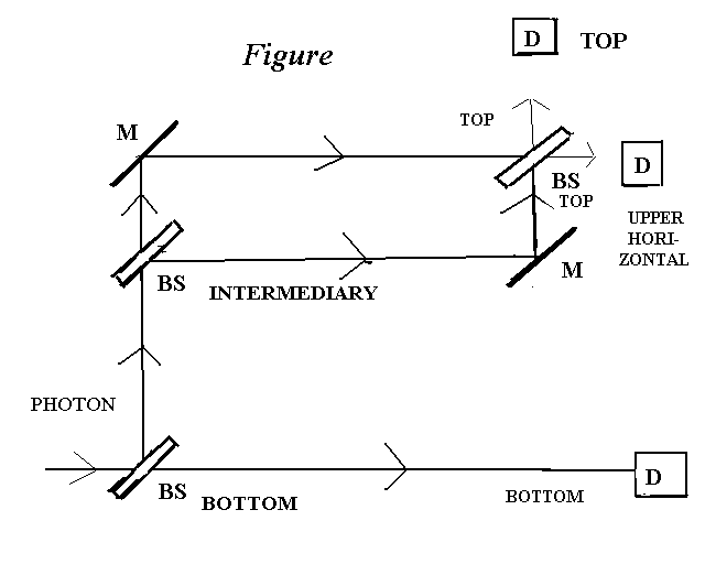
Figure 1: In the (slightly upgraded) Mach-Zehnder interference device there are three beam splitters (BS): the bottom one, the intermediary one, and the top one; there are two mirrors (M), and three detectors (D): the bottom one, the upper horizontal one, and the top (vertical) one. If the top beam splitter is removed, then we have the (slightly upgraded) Mach-Zehnder which-way device. The photon reaches the bottom beam splitter at the initial moment  $t_{i}\enspace$. It is the preparator as explained in subsection 8.1. For simplicity we assume that the possible detection in any of the three detectors takes place at one and the same moment  $t_{f}\enspace$. Let  $t_{i}\enspace$ be the moment when the photon passes the intermediary beam splitter. Naturally,  $t_{i}<t_{0}<t_{f}\enspace$. There are two observables: Let the observable  $B\enspace$ be defined at  $t_{i}\enspace$. It has two eigen-events:  $Q_{h}\enspace$, transmission through the bottom BS and propagation towards the bottom detector, and  $Q_{v}\enspace$ reflection at the bottom BS and propagation upwards towards the intermediary BS. The other observable  $B_{0}\enspace$ is defined at  $t_{0}\enspace$. It has three eigen-events:  $Q_{lh}\enspace$ lower horizontal propagation towards the bottom detector,  $Q_{uh}\enspace$ propagation from the intermediary BS along the upper horizontal line, and  $Q_{v}\enspace$, propagation from the intermediary BS vertically upwards.

In spite of the interference in the top BS,  $B\enspace$ (see the caption of the Figure) is a ’simplest which-way’ observable and the experiment is a which-way one relative to  $B\enspace$ in the sense of Section 5. Namely, due to the interference, there are only two detections (with probability one half each): in the bottom and in the top detector. If we manipulate the bottom BS as a preparator (cf subsection 8.1), then one can easily see that the necessary and sufficient condition in Theorem 1 is satisfied. On account of the simplicity of the experiment, one can argue also without Theorem 1 as follows.

Let the localization events be  $P_{b}\enspace$ in the bottom detector and  $P_{t}\enspace$ in the top one respectively. Since  $U(t_{f}-t_{i})^{{\dagger}}P_{b}U(t_{f}-t_{i})=Q_{h}\enspace$, and  $U(t_{f}-t_{i})^{{\dagger}}P_{t}U(t_{f}-t_{i})=Q_{v}\enspace$ (the Mach-Zehnder interference device is time-reversal symmetric), we can attach equal eigenvalues (which are anyway not important here) to  $A\enspace$ and  $B\enspace$, and obtain  $B=A^{r}(t_{i})\enspace$. Thus, we are dealing with a ’simplest which-way’ experiment in relation to  $B\enspace$. But ut is not particle-like behavior in the sense of Bohr because the photon is not localized all along  $t_{i}<t<t_{f}\enspace$; it exhibits wave-like behavior in the interval  $t_{0}\leq t<t_{f}$.

This discussion gives rigorous justification to the intuitive inference from the Figure that if the photon ends up in the bottom (top) detector, it had to come from its transmission through (reflection at) the bottom BS.

The experiment is an interference one with respect to the observable  $B_{0}\enspace$ (see the Caption). This is so because of the interference in the top BS.

Let us define the function (coarsening)  $B^{\prime}_{0}\enspace$ of  $B_{0}\enspace$ that keeps  $Q_{lh}\enspace$ as one of its eigen-events and has  $\Big{(}Q_{uh}+Q_{v}\Big{)}\enspace$ as the (only) other. The experiment is a which-way one (again in spite of the interference in the top BS) in relation to  $B^{\prime}_{0}\enspace$. It is not called ’simplest’ because this observable is defined at  $t_{0}\enspace$, and not at  $t_{i}$.

9.2 The Slightly Upgraded Mach-Zehnder Which-Way Device

Now the observable  $B\enspace$ is not the ’simplest which-way’ one. Namely, the condition in Theorem 1 is not satisfied as seen from the fact that  $Q_{v}\enspace$ does not lead with certainty to one detector localization.

Incidentally, the Figure and classical intuition would suggest that both the state of reaching the top detector and that of reaching the upper horizontal one ’come from’ the photon state  $\mid~{}\!\!\!{\phi_{v}}~{}\!\!\rangle\enspace$ corresponding to  $Q_{v}\enspace$ ( $Q_{v}\mid~{}\!\!\!{\phi_{v}}~{}\!\!\rangle=\mid~{}\!\!\!{\phi_{v}}~{}\!\!\rangle\enspace$). But this is a false conclusion because ’come from’ should mean quantum-mechanically the application of  $U(t_{f}-t)\enspace$. Or equivalently,  $\mid~{}\!\!\!{\phi_{v}}~{}\!\!\rangle\enspace$ should be obtained from the two mentioned final states by application of  $U(t_{f}-t)^{{\dagger}}\enspace$. But a unitary operator cannot map orthogonal states into one and the same one.

On the other hand, it is seen that  $U(t_{f}-t_{i})Q_{v}U(t_{f}-t_{i})^{{\dagger}}=P_{t}+P_{uh}\enspace$, and  $P_{uh}\enspace$ is the event of localization in the upper horizontal detector. Further,  $U(t_{f}-t_{i})Q_{h}U(t_{f}-t_{i})^{{\dagger}}=P_{b}\enspace$. Thus, if we take the function (or coarsening)  $f(A)\enspace$ of the measured observable  $A\enspace$ defined by the right-hand-sides, which is simultaneously also measured in the measurement of  $A\enspace$, then  $B^{f}\equiv U(t_{f}-t_{i})BU(t_{f}-t_{i})^{{\dagger}}=f(A)\enspace$. Since obviously  $[f(A),A]=0\enspace$, the condition in Theorem 2 is satisfied. Therefore,  $B\enspace$ is a ’simplest which-way’ observable for  $f(A)$.

As to  $B_{0}\enspace$, the condition in Theorem 1 makes it obvious that it is a ’simplest which-way’ observable for  $A\enspace$. But again it is not so in the sense of Bohr, because  $B_{0}\enspace$ is defined at the moment  $t_{0}\enspace$, and not at the initial moment.

10 What is Really Happening?

In an attempt to comprehend what was ’real’ for Bohr, let us read another quotation from him [26]

Quote BOHR6: ”As a more appropriate way of expression I advocate the application of the word phenomenon exclusively to refer to the observations obtained under specified circumstances, including an account of the whole experimental arrangement.(The italics are Bohr’s.)

I think that by ”phenomenon” Bohr means a real phenomenon, i. e., that this is where ’reality’ enters the scene in the view of Bohr.

The retrospective observable  $A^{r}(t)\enspace$ in the visualization theory of Sections 3-7 is primarily a mathematical construction, an ’evolving’ backward in time of the real observable  $A\enspace$. Even when the condition in Theorem 1 is satisfied, and we have the possibility of a visualization in a ’simplest which-result’ experiment, the eigen-events  $P^{r}_{n}\enspace$ do not really occur, not even in the Bohrian sense. They are only imagined or visualized to create a quasi-classical picture about what is going on within the experiment on hand.

This is particularly clear in Wheeler’s delayed-choice experiments, in which (both in the two-slit [25] and in the Mach-Zehnder [13] cases) the choice whether the experiment is going to be the ’which-way’ one or the ’interference’ one is made after the photon has passed the two slits (or the first beam splitter). Thus, whether the photon is going one way or both ways appears to be decided backwards in time. Obviously, these are not real events happening in nature.

Turning to Bohr’s forbiddance to combine visualizations from complementary experiments, contained in the complementarity principle, it seems a justified warning that should save us from taking the visualizations too seriously, i. e., as if they were real occurrences in nature, and thus different aspects of reality that should be combined into a complete picture. In quantum-mechanical insight all aspects are present simultaneously. If one overemphasizes and even falsifies two distinct aspects (the wave-like and the particle-like one in Bohr’s approach), it is natural that they become incompatible.

11 Assessment

A good deal of physical evaluation of wave-particle complementarity in the Bohrian way was accomplished during the critical derivation in sections 3-7 because it was done purposely pointing out the arbitrary or imaginary steps.

Now I’ll pay additional attention only to the (most important) case of ’simplest interference-which result’ experiment, in particular when  $A^{r}(t_{i})\enspace$ is physically meaningful.

Let me discuss the first illusion (the first drastic imagined step of changes, cf Section 5, second passage). As far as the experiment is concerned, the initial state  $\rho(t_{i})\enspace$ can be replaced by the butchered mixture with respect to the ’back-evolved’ observable  $A^{r}(t_{i})\enspace$ (cf (8a)). But, if there is coherence (cf Definition 1), then the ’which-result’ visualization in case the individual experiment gives one of these results, grossly violates the coherence, which, from the point of view of the ’reality-of-state’ approach, to which this author adheres, is a serious falsification of reality.

Thus, in case of the Mach-Zehnder which-way device (cf Subsection 8.1) with a coherent initial state (cf (13a)), the Bohrian particle-like aspect creates the illusion that the photon takes one of the paths. This violates grossly the coherence.

John Bell had apparently strong feelings about this as it is clear from his term ”butchered” state vector for  $\rho_{M}(t_{i})\enspace$ [18].

Let me turn to the second illusion (the second drastic imagined step of changes). Classically, interpretation of  $\rho(t_{i})_{M}\enspace$ as a simple mixture would mean that there is, e. g., a subensemble  $\rho(t_{i})_{M}^{n}\enspace$ in it which has the sharp value in question, and the individual quantum system belongs to this subensemble. Then, at first glance, the ’which-result visualization’ might appear to correspond to reality.

This argument may stem from a Bohrian devotedness to classical physics. From the point of view of the ’reality-of-state’ approach, this is an unacceptable prejudice. Namely, as well known, even if the density operator has no more than a two-dimensional range, there are infinitely many decompositions into density operators, i. e., it can be written in that many ways as a mixture. Quantum-mechanically none of them has a privileged role, which would enable one interpret it as the real state of affairs (as far as decomposition of ensemble into individual-system states is concerned).

Neither this point has escaped Bell’s attention as seen from his words [27]:

Quote BELL2: ”The idea that elimination of coherence, in one way or another, implies the replacement of ’and’ by ’or’ is a very common one among solvers of the ’measurement problem’. It has always puzzled me.”

Thus, the Bohrian approach in terms of complementary particle-like and wave-like experiments does not reveal two, mutually exclusive, aspects of the state  $\rho(t_{i})\enspace$. It gives a completely distorted view. It has very little to do with reality. (Though, it does give a simplified semi-classical understanding of what is going on in the experiment in partial agreement with quantum mechanics.)

As to merits of the present study (if any), I would like to quote Fagundes [28]:

Quote FAGUNDES: ”… physics progresses by increasing degrees of abstraction. This is only natural since ’concrete’ ideas are just those of our too limited ordinary sense experience.”

I think, these words are applicable, to some extent, also to the slight progress achieved by deriving a sharp and extended form of ’interference-which-result’ complementarity from quantum mechanics in this article.

12 Concluding Remarks

The derivation in sections 3-7 follows Bohr’s endeavor to envelop the understanding of a quantum experiment in classical physics as in a chocolate coating. This is not surprising when one takes into account what a low opinion Bohr had of the quantum formalism. I’ll give two excerpts to illustrate this claim. The first is from Saunders [29].

Quote SAUNDERS: ”The quantum formalism is only an abstract calculus. As we have seen, Bohr made this point over and over again.” (Italics by Saunders)

On Bohr’s suspicion about the quantum formalism we have similar words by Heisenberg [30]

Quote HEISENBERG: ”I noticed that mathematical clarity had in itself no virtue for Bohr. He feared that the formal mathematical structure would obscure the physical core of the problem,…”

Reichenbach [16] made a variation on Bohr’s idea of visualization by introducing ’interphenomena’.

Fagundes [28], probably laboring under the burden of lack of sufficient reality in both Bohr’s and Reichenbach’s concepts, suggested to replace visualization by literally nothing. (A consistently positivistic point of view, so it appears.)

Holladay’s ”which-value-interference complementarity” approach [31] is closest to mine. (I was even influenced by his terminology.)

I am certain that there are other praiseworthy related endeavors that have escaped my attention.

Murdoch, in his detailed study of Bohr [32], writes (beginning of p. 68):

Quote MURDOCH1: ”Bohr came to hold that the wave and particle models are equally necessary for a complete description of the real nature of micro-physical entities - the symmetry thesis, as I shall call it.”

Later on (in the second passage of p. 79) he writes:

Quote MURDOCH2: ”The symmetry thesis, then, is difficult to sustain, and with it the thesis of wave-particle complementarity. The thesis has lost the palliative value it once had, and has now merely a historical significance.” (Emphasis by F. H..)

The present study confirms this dismissal of Bohr’s complementarity principle on part of Murdoch (who, as it seems, has studied Bohr thoroughly). Present-day research on the foundations of quantum mechanics does not need palliation. Its aim is to understand quantum reality as it is.

Finally, I would like to point out that Bohr and the Copenhagen interpretation [33] caused a substantial delay in the historical development of the foundations of quantum mechanics. Bohr’s own words [34] bear witness to this claim.

Quote BOHR7: ”There is no quantum world. There is only an abstract quantum physical description. It is wrong to think that the task of physics is to find out how nature is. Physics concerns what we can say about nature.”

By now it must be obvious to the reader that the author’s attitude in the analysis in this article is a rebelion against this view of Bohr. The reality-of-state approach, to which the author is partial, stipulates precisely the opposite: however abstract, we must take the quantum-mechanical description of experiments seriously because it reveals how nature is. And no lesser goal is worthy of our efforts. We should be able to ”say about nature” how it really is though only in an approximation that should be as good as possible.

I think that Gell-Mann gave an impressive criticism of Bohr [35]:

Quote GELL-MANN: ”The fact that an adequate philosophical presentation has been so long delayed is no doubt caused by the fact that Niels Bohr brainwashed a whole generation of theorists into thinking that the job was done fifty years ago”

Landsman says [36] (p. 214) ”Beller [37] went further than any critic before or after her by portraying Bohr not as the Gandhi of 20th century physics (as in Pais, 1991 [38]), but rather as its Stalin, a philosophical dilettante who knew no mathematics and hardly even followed the physics of his day, but who nonetheless managed to stifle all opposition by a combination of political manoeuvring, shrewd rhetoric, and spellbinding both his colleagues and the general audience by the allegedly unfathomable depth of his thoughts (which, according to Beller, were actually incoherent and inconsistent)” (italics by F. H.).

Landsman then comments as follows: ”Despite Beller’s meticulous and passionate arguments, we do not actually believe Bohr’s philosophy of quantum mechanics was such a great muddle after all.”

Let me point out, at the end, that in spite of the mentioned delay, it seems to me that Bohr has done mankind an invaluable service by saving it from being hopelessly lost in a labyrinth searching for objective quantum mechanics at an early stage. Thus, he made possible the unparalleled swift development of quantum mechanics in atomic, molecular, solid-state etc. physics, i. e., a rapid and immense progress of quantum mechanics as a practical science and no less of quantum technology.

Appendix A: Proof of Theorem 1

Proof Necessity If the retrospective observable  $A^{r}(t)\enspace$ has a physical meaning, then one can take  $B(t)\equiv A^{r}(t),\enspace$ and the bijection is the identity map. The required property obviously holds.

Sufficiency Let  $B(t)=\sum_{k}b_{k}Q_{k}(t)\enspace$ be an observable with physical meaning, and let  $\{\mid~{}\!\!\!{\phi(t)}~{}\!\!\rangle_{k,l_{k}}:\forall k,\forall l_{k}\}\enspace$ be a complete orthonormal eigen-basis of  $B(t)\enspace$ satisfying

$$\forall k:\quad\sum_{l_{k}}\mid~{}\!\!\!{\phi(t)}~{}\!\!\rangle_{k,l_{k}}\langle~{}\!\!{\phi(t)}~{}\!\!\!\mid_{k,l_{k}}=Q_{k}(t).$$

This makes the vectors  $\mid~{}\!\!\!{\phi(t)}~{}\!\!\rangle_{k,l_{k}}\enspace$ eigen-vectors of  $B(t)\enspace$ corresponding to the eigenvalues  $b_{k}\enspace$, and the index  $l_{k}\enspace$ enumerates the multiplicity (possible degeneracy) of the eigenvalue  $b_{k}\enspace$ of  $B\enspace$.

Further, one can define

$$\forall k,l_{k}:\quad\mid~{}\!\!\!{\psi(t_{f})}~{}\!\!\rangle_{k,l_{k}}\equiv U(t_{f}-t)\mid~{}\!\!\!{\phi(t)}~{}\!\!\rangle_{k,l_{k}}.$$

On account of the unitarity of  $U(t_{f}-t)\enspace$, also the basis  $\{\mid~{}\!\!\!{\psi(t_{f})}~{}\!\!\rangle_{k,l_{k}}:\forall k,\forall l_{k}\}\enspace$ is orthonormal and complete.

Relations (A.1) imply that each state  $\mid~{}\!\!\!{\phi(t)}~{}\!\!\rangle_{k,l_{k}}\enspace$ has the property  $Q_{k}(t),\enspace$ and, since we assume validity of the condition in Theorem 1, the result of the measurement of  $A\enspace$ in the corresponding final state  $\mid~{}\!\!\!{\psi(t_{f})}~{}\!\!\rangle_{k,l_{k}}\enspace$ is certainly  $a_{n(k)},\enspace$ i. e.,

$$\forall k,l_{k}:\quad{\rm tr}(P_{n(k)}\mid~{}\!\!\!{\psi}~{}\!\!\rangle_{k,l_{k}}\langle~{}\!\!{\psi}~{}\!\!\!\mid_{k,l_{k}})=1.$$

We can rewrite this as

$$\forall k,l_{k}:\quad\Big{(}\langle~{}\!\!{\psi}~{}\!\!\!\mid_{k,l_{k}}P_{n(k)}\Big{)}\Big{(}P_{n(k)}\mid~{}\!\!\!{\psi}~{}\!\!\rangle_{k,l_{k}}\Big{)}=1,$$

implying

$$\forall k,l_{k}:\quad\Big{(}\langle~{}\!\!{\psi}~{}\!\!\!\mid_{k,l_{k}}P_{n(k)}^{\perp}\Big{)}\Big{(}P_{n(k)}^{\perp}\mid~{}\!\!\!{\psi}~{}\!\!\rangle_{k,l_{k}}\Big{)}=0,$$

where  $P_{n(k)}^{\perp}\equiv I-P_{n(k)},\enspace$  $I\enspace$ being the identity operator. Further, one obtains  $P_{n(k)}^{\perp}\mid~{}\!\!\!{\psi}~{}\!\!\rangle_{k,l_{k}}=0\enspace$ (due to positive definiteness of the norm), and

$$\forall k,l_{k}:\quad P_{n(k)}\mid~{}\!\!\!{\psi}~{}\!\!\rangle_{k,l_{k}}=\mid~{}\!\!\!{\psi}~{}\!\!\rangle_{k,l_{k}},$$

implying

$$\forall k,l_{k}:\quad P_{n(k)}\mid~{}\!\!\!{\psi}~{}\!\!\rangle_{k,l_{k}}\langle~{}\!\!{\psi}~{}\!\!\!\mid_{k,l_{k}}=\mid~{}\!\!\!{\psi}~{}\!\!\rangle_{k,l_{k}}\langle~{}\!\!{\psi}~{}\!\!\!\mid_{k,l_{k}}.$$

Summing out  $l_{k}\enspace$ for each value of  $k,\enspace$ and utilizing (A.2) and (A.1), one obtains

$$\forall k:\quad P_{n(k)}\Big{(}U(t_{f}-t)Q_{k}(t)U(t_{f}-t)^{{\dagger}}\Big{)}=U(t_{f}-t)Q_{k}(t)U(t_{f}-t)^{{\dagger}}.$$

On the other hand, we have, in view of (5b) and (A.3),

$$\forall k:\quad P_{n(k)}=P_{n(k)}I=P_{n(k)}\Big{[}\sum_{k^{\prime}}\Big{(}U(t_{f}-t)Q_{k^{\prime}}(t)U(t_{f}-t)^{{\dagger}})\Big{)}\Big{]}=$$

$$P_{n(k)}\Big{[}\sum_{k^{\prime}}\Big{(}P_{n(k^{\prime})}U(t_{f}-t)Q_{k^{\prime}}(t)U(t_{f}-t)^{{\dagger}})\Big{)}\Big{]}=P_{n(k)}\Big{(}U(t_{f}-t)Q_{k}(t)U(t_{f}-t)^{{\dagger}}\Big{)}.$$

Relations (A.3) and (A.4) imply

$$\forall k:\quad U(t_{f}-t)Q_{k}(t)U(t_{f}-t)^{{\dagger}}=P_{n(k)},$$

which is equivalent to

$$\forall k:\quad Q_{k}(t)=P_{n(k)}^{r}(t)$$

(cf (4b)). Hence,  $B(t)=A^{r}(t).$ $\Box$

Appendix B: Proof of Theorem 2

First we prove a lemma.

A.Lemma The commutation condition (12) is equivalent to

$$\forall(k\not=k^{\prime}),\enskip\forall n:\quad Q_{k}^{f}P_{n}Q_{k^{\prime}}^{f}=0.$$

Proof On account of the well-known fact that two Hermitian operators with purely discrete spectra commute if and only if each eigen-projector of one commutes with each eigen-projector of the other, (12) implies (B.1). Conversely, utilizing the completeness relation (5b), which is obviously valid mutatis mutandis for the spectral eigen-projectors of  $B^{f}\enspace$, one can see that if (B.1) is valid, then

$$\forall k,n:\quad Q_{k}^{f}P_{n}=Q_{k}^{f}P_{n}I=\sum_{k^{\prime}}Q_{k}^{f}P_{n}Q_{k^{\prime}}^{f}=Q_{k}^{f}P_{n}Q_{k}^{f}.$$

Adjoining this, one obtains

$$\forall k,n:\quad P_{n}Q_{k}^{f}=Q_{k}^{f}P_{n}Q_{k}^{f}.$$

These two relations imply (12). $\Box$

Proof of Theorem 2 Sufficiency of (12) for ’which-result’ behavior. Straightforward calculation shows that, owing to (12), A.Lemma, and (B.1),

$$\forall n:\quad{\rm tr}\Big{(}\rho(t_{f})P_{n}\Big{)}={\rm tr}\Big{(}I\rho(t_{f})IP_{n}\Big{)}=$$

$$\sum_{k}\sum_{k^{\prime}}{\rm tr}\Big{(}Q_{k}^{f}\rho(t_{f})Q_{k^{\prime}}^{f}P_{n}\Big{)}=\sum_{k}\sum_{k^{\prime}}{\rm tr}\Big{(}\rho(t_{f})Q_{k^{\prime}}^{f}P_{n}Q_{k}^{f}\Big{)}=$$

$$\sum_{k}{\rm tr}\Big{(}Q_{k}^{f}\rho(t_{f})Q_{k}^{f}P_{n}\Big{)}={\rm tr}\Big{(}\rho(t_{f})_{M,B}P_{n}\Big{)}.$$

Necessity of (12) for ’which-result’ behavior and proof of claim B). Now we argue that if (12) is not valid, then  $B\enspace$ is an ’interference’ observable. (In this way we prove both that which-result behavior implies (12), and claim B).)

Let (12) not be valid. Then  $\exists k,n,k^{\prime}\enspace$ such that  $Q_{k}^{f}P_{n}Q_{k^{\prime}}^{f}\not=0\enspace$ (cf A.Lemma). Let, further,

$$Q_{k}^{f}\equiv\sum_{l_{k}}\mid~{}\!\!\!{l_{k}}~{}\!\!\rangle\langle~{}\!\!{l_{k}}~{}\!\!\!\mid,$$

and

$$Q_{k^{\prime}}^{f}\equiv\sum_{l_{k^{\prime}}}\mid~{}\!\!\!{l_{k^{\prime}}}~{}\!\!\rangle\langle~{}\!\!{l_{k^{\prime}}}~{}\!\!\!\mid$$

be projector decompositions into ray projectors (in terms of basis vectors defined by (B.2a) and (B.2b), though incompletely in general). Substitution of (B.2a) and (B.2b) in the inequality leads to  $\sum_{l_{k}}\sum_{l_{k^{\prime}}}\mid~{}\!\!\!{l_{k}}~{}\!\!\rangle\langle~{}\!\!{l_{k}}~{}\!\!\!\mid P_{n}\mid~{}\!\!\!{l_{k^{\prime}}}~{}\!\!\rangle\langle~{}\!\!{l_{k^{\prime}}}~{}\!\!\!\mid\not=0.\enspace$ Hence, there must exist special values  $l_{k}\enspace$ and  $l_{k^{\prime}}\enspace$ such that

$$\langle~{}\!\!{l_{k}}~{}\!\!\!\mid P_{n}\mid~{}\!\!\!{l_{k^{\prime}}}~{}\!\!\rangle\not=0.$$

Let

$$\mid~{}\!\!\!{l_{k},t_{i}}~{}\!\!\rangle\equiv U(t_{f}-t_{i})^{{\dagger}}\mid~{}\!\!\!{l_{k}}~{}\!\!\rangle,\quad\mid~{}\!\!\!{l_{k^{\prime}},t_{i}}~{}\!\!\rangle\equiv U(t_{f}-t_{i})^{{\dagger}}\mid~{}\!\!\!{l_{k^{\prime}}}~{}\!\!\rangle.$$

Finally, let  $\alpha,\enskip\beta\enspace$ be non-zero complex numbers such that  $|\alpha|^{2}+|\beta|^{2}=1\enspace$. We define the initial state

$$\rho(t_{i})\equiv\Big{(}\alpha\mid~{}\!\!\!{l_{k},t_{i}}~{}\!\!\rangle+\beta\mid~{}\!\!\!{l_{k^{\prime}},t_{i}}~{}\!\!\rangle\Big{)}\Big{(}\alpha*\langle~{}\!\!{l_{k},t_{i}}~{}\!\!\!\mid+\beta*\langle~{}\!\!{l_{k^{\prime},t_{i}}}~{}\!\!\!\mid\Big{)},$$

where the asterisk denotes complex conjugation. Then the final state is

$$\rho(t_{f})=\Big{(}\alpha\mid~{}\!\!\!{l_{k}}~{}\!\!\rangle+\beta\mid~{}\!\!\!{l_{k^{\prime}}}~{}\!\!\rangle\Big{)}\Big{(}\alpha^{*}\langle~{}\!\!{l_{k}}~{}\!\!\!\mid+\beta^{*}\langle~{}\!\!{l_{k^{\prime}}}~{}\!\!\!\mid\Big{)}.$$

As to the ’unbutchered’ and the ’butchered’ states, (B.2a) and (B.2b) imply, as easily seen,

$${\rm tr}\Big{(}\rho(t_{f})P_{n}\Big{)}={\rm tr}\Big{(}I\rho(t_{f})IP_{n}\Big{)}=$$

$$\sum_{k^{\prime\prime}}{\rm tr}\Big{(}Q_{k^{\prime\prime}}^{f}\rho(t_{f})Q_{k^{\prime\prime}}^{f}P_{n}\Big{)}+\sum_{k^{\prime\prime}\not=k^{\prime\prime\prime}}{\rm tr}\Big{(}Q_{k^{\prime\prime}}^{f}\rho(t_{f})Q_{k^{\prime\prime\prime}}^{f}P_{n}\Big{)}=$$

$${\rm tr}\Big{(}\rho(t_{f})_{M,B}P_{n}\Big{)}+\alpha\beta*\langle~{}\!\!{l_{k^{\prime}}}~{}\!\!\!\mid P_{n}\mid~{}\!\!\!{l_{k}}~{}\!\!\rangle+\beta\alpha*\langle~{}\!\!{l_{k}}~{}\!\!\!\mid P_{n}\mid~{}\!\!\!{l_{k^{\prime}}}~{}\!\!\rangle.$$

It follows from (B.3) that this is different than  ${\rm tr}\Big{(}\rho(t_{f})_{M,B}P_{n}\Big{)},\enspace$ i. e., the experiment distinguishes the the ’unbutchered’ and the ’butchered’ states. Since  $B(t)\enspace$ and  $B^{f}\enspace$ are by assumption physically meaningful, so are, in principle, also the eigen-states  $\mid~{}\!\!\!{l_{k}}~{}\!\!\rangle\enspace$ and  $\mid~{}\!\!\!{l_{k^{\prime}}}~{}\!\!\rangle\enspace$ of  $B^{f}\enspace$. $\Box$

References

- [1] Herbut F., Vujičić M.: First-quantisation quantum-mechanical insight into the Hong-Ou-Mandel two-photon interferometer with polarizers and its role as a quantum eraser. Phys. Rev. A 56, 1-5 (1997)
- [2] Herbut, F.: On EPR-Type Entanglement in the Experiments of Scully et al. I. The Micromaser Case and Delayed-Choice Quantum Erasure. Found. Phys. 38, 1046-1064 (2008); arXiv:0808.3176
- [3] Herbut, F.: On EPR-Type Entanglement in the Experiments of Scully et al. II. Insight in the Real Random Delayed-Choice Erasure Experiment. arXiv:0808.3177
- [4] Einstein, A.: Remarks on the Essays Appearing in this Collective Volume. In: Schilpp, P. A. (ed.) Albert Einstein: Philosopher-Scientist. The Library of Living Philosophers Inc., Evanston, Illinois (1949), p. 674, last passage
- [5] Born, M.: The Restless Universe. Dover, New York (1951), p.283
- [6] Ghose, P., Home, D.: The Two-Prism Experiment and Wave-Particle Duality of Light. Found. Phys. 26, 943-953 (1996)
- [7] Rangwala, S., Roy, S.M.: Wave Behavior and Noncomplementary Particle Behavior in the Same Experiment. Phys. Lett. A 190, 1-4 (1994)
- [8] Ghose, P., Sinha Roy, M.N.: Confronting the Complementarity Principle in an Interference Experiment. Phy. Lett. A 161, 5-8 (1991)
- [9] Bohr, N.: Discussion with Einstein on Epistemological Problems in Atomic Physics. In: Schilpp, P. A. (ed.) Albert Einstein: Philosopher-Scientist. The Library of Living Philosophers Inc., Evanston, Illinois (1949). P. 222, the passage in the middle of the page
- [10] Nachman, P.: Mach-Zehnder Interferometer as an Instructional Tool. Am. J. Phys. 63, 39-43 (1995)
- [11] Bohr, N.: Natural Philosophy and Human Cultures. In: Atomic Physics and Human Knowledge. Wiley, New York (1958), p. 26
- [12] Bohr, N.: Discussion with Einstein on Epistemological Problems in Atomic Physics”. In: Schilpp, P. A. (ed.) Albert Einstein: Philosopher-Scientist. The Library of Living Philosophers Inc., Evanston, Illinois (1949), p. 210, end of first passage
- [13] Wheeler, J. A.: The ’past’ and the delayed-choice double-slit experiment. In: Marlow A. R. (ed). Mathematical Foundations of Quantum Theory. Academic Press, New York (1978), p. 32
- [14] Bohr, N.: Nature (Suppl.) 128, 691 (1931)
- [15] Schlosshauer, M.: arXiv: 0804.1609
- [16] Reichenbach, H.: Philosophic Foundations of Quantum Mechanics. Univ. California Press, Berkeley (1965)
- [17] Herbut, F.: A Quantum Measure of Coherence and Incompatibility. J. Phys. A: Math. Gen. 38, 2959-2974 (2005)
- [18] Bell, J.: Against ’Measurement’. Phys. World, August, p. 37, right column, second passage
- [19] Busch, P., Lahti, P.J., Mittelstaedt, P.: The Quantum Theory of Measurement. Lecture Notes in Physics, M2. Springer Verlag, Berlin (1991).
- [20] Herbut, F.: Delayed-Choice Experiments and Retroactive Apparent Occurrence in the Quantum Theory of Measurement. Found. Phys. 24, 117-137 (1994), section 2
- [21] Herbut, F.: On Retroactive Occurrence and Twin Events in Quantum Mechanics. Found. Phys. Lett. 9, 437-446 (1996)
- [22] Bacciagaluppi, G., Valentini, A.: Quantum Theory at the Crossroads. Cambridge Univ. Press, Cambridge (2006). arXiv:quant-ph/0609184
- [23] Kim Y.-H., Yu R., Kulik S. P., Shih Y., Scully M. O.: Delayed ”choice” quantum eraser. Phys. Rev. Lett. 84, 1-5 (2000); also arXiv: quant-ph/9903047
- [24] Grangier, P., Roger, G., Aspect, A.: Experimental Evidence for a Photon Anticorrelation Effect on a Beam Splitter: A New Light on Single-Photon Interferences. Europhys. Lett. 1, 173-179 (1986)
- [25] Wheeler J. A.: The ’past’ and the delayed-choice double-slit experiment. In: Marlow A. R. ed. Mathematical Foundations of Quantum Theory. Academic Press, New York (1978), p. 11
- [26] Bohr, N.: Discussion with Einstein on Epistemological Problems in Atomic Physics. In: Schilpp, P. A. (ed.) Albert Einstein: Philosopher-Scientist. The Library of Living Philosophers Inc., Evanston, Illinois (1949). Pp. 237-238
- [27] Bell, J.: Against ’Measurement’. Phys. World, August, p. 36, right column, fourth passage from below
- [28] Fagundes, H.V.: The Discontinuous Spatiality of Quantum Mechanical Objects. arXiv:quant-ph/0504125v2
- [29] Saunders, S.: Complementarity and Scientific Rationality. Found. Phys. 35, 417-447 (2005), p. 432
- [30] Rosenthal, S. (ed.): Niels Bohr, His Life and Work as Seen by his Friends and Colleagues. New York (1967), p. 98
- [31] Holladay, W.G.: The Nature of Particle-Wave Complementarity. Am. J. Phys. 66, 27-33 (1998)
- [32] Murdoch, D.: Niels Bohr’s Philosophy of Physics. Cambridge Univ. Press, Cambridge (1987)
- [33] Stapp, H.P.: The Copenhagen Interpretation. Am. J. Phys. 40, 1098-1116 (1972)
- [34] Petersen, A.: The Philosophy of Niels Bohr. The Bulletin of the Atomic Scientists. September (1963), p. 8
- [35] Gell-Mann, M.: The Nature of the Physical World. Wiley, New York (1979)
- [36] Landsman, N.P.: When Champions Meet: Rethinking the Bohr-Einstein Debate. Stud. Hist. Phil. Mod. Phys. 37, 212-242 (2006), pp. 214-215
- [37] Beller, M.: Quantum Dialogue. Univ. Chicago Press, Chicago (1999)
- [38] Pais, A.: Niels Bohr’s Times: In Physics, Philosophy, and Polity. Oxford Univ. Press, Oxford (1991)