Induction of Word and Phrase Alignments for Automatic Document Summarization

Abstract

Current research in automatic single document summarization is dominated by two effective, yet naïve approaches: summarization by sentence extraction, and headline generation via bag-of-words models. While successful in some tasks, neither of these models is able to adequately capture the large set of linguistic devices utilized by humans when they produce summaries. One possible explanation for the widespread use of these models is that good techniques have been developed to extract appropriate training data for them from existing document/abstract and document/headline corpora. We believe that future progress in automatic summarization will be driven both by the development of more sophisticated, linguistically informed models, as well as a more effective leveraging of document/abstract corpora. In order to open the doors to simultaneously achieving both of these goals, we have developed techniques for automatically producing word-to-word and phrase-to-phrase alignments between documents and their human-written abstracts. These alignments make explicit the correspondences that exist in such document/abstract pairs, and create a potentially rich data source from which complex summarization algorithms may learn. This paper describes experiments we have carried out to analyze the ability of humans to perform such alignments, and based on these analyses, we describe experiments for creating them automatically. Our model for the alignment task is based on an extension of the standard hidden Markov model, and learns to create alignments in a completely unsupervised fashion. We describe our model in detail and present experimental results that show that our model is able to learn to reliably identify word- and phrase-level alignments in a corpus of $\langle$document, abstract$\rangle$ pairs.

1 Introduction and Motivation

1.1 Motivation

We believe that future success in automatic document summarization will be made possible by the combination of complex, linguistically motivated models and effective leveraging of data. Current research in summarization makes a choice between these two: one either develops sophisticated, domain-specific models that are subsequently hand-tuned without the aid of data, or one develops naïve general models that can be trained on large amounts of data (in the form of corpora of document/extract or document/headline pairs). One reason for this is that currently available technologies are only able to extract very coarse and superficial information that is inadequate for training complex models. In this paper, we propose a method to overcome this problem, by automatically generating word-to-word and phrase-to-phrase alignments between documents and their human-written abstracts.

To facilitate discussion and to motivate the problem, we show in Figure 1 a relatively simple alignment between a document fragment and its corresponding abstract fragment from our corpus. In this example, a single abstract sentence (shown along the top of the figure) corresponds to exactly two document sentences (shown along the bottom of the figure). If we are able to automatically generate such alignments, one can envision the development of models of summarization that take into account effects of word choice, phrasal and sentence reordering, and content selection. Such models could be simultaneously linguistically motivated and data-driven. Furthermore, such alignments are potentially useful for current-day summarization techniques, including sentence extraction, headline generation and document compression.

Figure 1: Example alignment of a single abstract sentence with two document sentences.

A close examination of the alignment shown in Figure 1 leads us to three observations about the nature of the relationship between a document and its abstract, and hence about the alignment itself:

• Alignments can occur at the granularity of words and of phrases.

• The ordering of phrases in an abstract can be different from the ordering of phrases in the document.

• Some abstract words do not have direct correspondents in the document, and many document words are never used in an abstract.

In order to develop an alignment model that could potentially recreate such an alignment, we need our model to be able to operate both at the word level and at the phrase level, we need it to be able to allow arbitrary reorderings, and we need it to be able to account for words on both the document and abstract side that have no direct correspondence. In this paper, we develop an alignment model that is capable of learning all these aspects of the alignment problem in a completely unsupervised fashion.

1.2 Shortcomings of current summarization models

Current state of the art automatic single-document summarization systems employ one of three techniques: sentence extraction, bag-of-words headline generation, or document compression. Sentence extraction systems take full sentences from a document and concatenate them to form a summary. Research in sentence extraction can be traced back to work in the mid fifties and late sixties by Luhn [Luhn,1956] and Edmundson [Edmundson,1969]. Recent techniques are startlingly not terribly divergent from these original methods; see [Mani and Maybury,1999, Marcu,2000, Mani,2001] for a comprehensive overview. Headline generation systems, on the other hand, typically extract individual words from a document to produce a very short headline-style summary; see [Banko, Mittal, and Witbrock,2000, Berger and Mittal,2000, Schwartz, Zajic, and Dorr,2002] for representative examples. Between these two extremes, there has been a relatively modest amount of work in sentence simplification [Chandrasekar, Doran, and Bangalore,1996, Mahesh,1997, Carroll et al.,1998, Grefenstette,1998, Jing,2000, Knight and Marcu,2002] and document compression [Daumé III and Marcu,2002, Daumé III and Marcu,2004, Zajic, Dorr, and Schwartz,2004] in which words, phrases and sentences are selected in an extraction process.

While such approaches have enjoyed some success, they all suffer from modeling shortcomings. Sentence extraction systems and document compression models make unrealistic assumptions about the summarization task (namely, that extraction is sufficient, and that sentences are the appropriate level of granularity). Headline generation systems employ very weak models that make an incorrect bag-of-words assumption. This assumption allows such systems to learn limited transformations to produce headlines from arbitrary documents, but such transformations are not nearly complex enough to adequately model anything beyond indicative summaries at a length of around ten words. Bag of words models can learn what the most important words to keep in a headline are, but say nothing about how to structure them in a well-formed, grammatical headline.

In our own work on document compression models [Daumé III and Marcu,2002, Daumé III and Marcu,2004], both of which extend the sentence compression model of Knight and Marcu [Knight and Marcu,2002], we assume that sentences and documents can be summarized exclusively through deletion of contiguous text segments. In Knight and Marcu’s data, we found that from a corpus of $39,060$ abstract sentences, only $1067$ were created from corresponding document sentences via deletion of contiguous segments. In other words, only $2.7\%$ of the sentences in real $\langle$document, abstract$\rangle$ pairs can be explained by the model proposed by Knight and Marcu [Knight and Marcu,2002]. Such document compression models do not explain the rich set of linguistic devices employed, for example, in Figure 1.

1.3 Prior work on alignments

In the sentence extraction community, there exist a wide variety of techniques for (essentially) creating alignments between document sentences and abstract sentences [Kupiec, Pedersen, and Chen,1995, Teufel and Moens,1997, Marcu,1999]; see also [Barzilay and Elhadad,2003, Quirk, Brockett, and Dolan,2004] for work describing alignments for the monolingual paraphrasing task. These techniques typically take into account information such as lexical overlap, synonymy, ordering, length, discourse structure, and so forth. The sentence alignment problem is a comparatively simple problem to solve and current approaches work quite well. Unfortunately, these alignments are the least useful, as they can only be used to train sentence extraction systems.

In the context of headline generation, simple statistical models are used for aligning documents and headlines [Banko, Mittal, and Witbrock,2000, Berger and Mittal,2000, Schwartz, Zajic, and Dorr,2002], based on IBM Model 1 [Brown et al.,1993]. These models treat documents and headlines as simple bags of words and learn probabilistic word-based mappings between the words in the documents and the words in the headlines. Such mappings can be considered word-to-word alignments, but as our results show (see Section 5), these models are too weak for capturing the sophisticated operations that are employed by humans in summarizing texts.

To date, there has been very little work on the word alignment task in the context of summarization. The most relevant work is that of Jing [Jing,2002], in which a hidden Markov alignment model is applied to the task of identifying word and phrase-level correspondences between documents and abstracts. Unfortunately, this model is only able to align words that are identical up to their stems, and thus suffers from a problem of recall. This also makes it ill-suited to the task of learning how to perform abstraction, in which one would desire to know how words get changed. For example, Jing’s model cannot identify any of the following alignments from Figure 1: (Connecting Point $\leftrightarrow$ Connecting Point Systems), (Mac $\leftrightarrow$ Macintosh), (retailer $\leftrightarrow$ seller), (Macintosh $\leftrightarrow$ Apple Macintosh systems) and (January 1989 $\leftrightarrow$ last January).

Word alignment (and, to a lesser degree, phrase alignment) has been an active topic of research in the machine translation community. Based on these efforts, one might be initially tempted to use readily-available alignment models developed in the context of machine translation, such as GIZA++ [Och and Ney,2003] to obtain word-level alignments in $\langle$document, abstract$\rangle$ corpora. However, as we will show (Section 5), the alignments produced by such a system are inadequate for the $\langle$document, abstract$\rangle$ alignment task.

1.4 Paper structure

In this paper, we describe a novel, general model for automatically inducing word- and phrase-level alignments between documents and their human-written abstracts. Beginning in Section 2, we will describe the results of human annotation of such alignments. Based on this annotation, we will investigate the empirical linguistic properties of such alignments, including lexical transformations and movement. In Section 3, we will introduce the statistical model we use for deriving such alignments automatically. The inference techniques are based on those of semi-Markov models, extensions of hidden Markov models that allow for multiple simultaneous observations.

After our discussion of the model structure and algorithms, we discuss the various parameterizations we employ in Section 4. In particular, we discuss three distinct models of movement, two of which are well-known in the machine translation alignment literature, and a third one that exploits syntax in a novel, “light” manner. We also discuss several models of lexical rewrite, based on identities, stems, WordNet synonymy and automatically induced lexical replacements. In Section 5, we present experimental results that confirm that our model is able to learn the hidden structure in our corpus of $\langle$document, abstract$\rangle$ pairs. We compare our model against well-known alignment models designed for machine translation, as well as a state of the art alignment model specifically designed for summarization [Jing,2002]. Additionally, we discuss errors that the model currently makes, supported by some relevant examples and statistics. We conclude with some directions for future research (Section 6).

2 Human-produced Alignments

 

[]Ziff-Davis corpus statistics

  Sub-corpus Annotated Abstracts Documents Abstracts Documents Documents $2033$ $45$ Sentences $13k$ $82k$ $244$ $2k$ Words $261k$ $2.5m$ $6.4k$ $49k$ Unique words $14k$ $42k$ $1.9k$ $5.9k$ $45k$ $6k$ Sentences/Doc $6.28$ $40.83$ $5.42$ $45.3$ Words/Doc $128.52$ $1229.71$ $142.33$ $1986.16$ Words/Sent $20.47$ $28.36$ $26.25$ $24.20$

In order to decide how to design an alignment model and to judge the quality of the alignments produced by a system, we first need to create a set of “gold standard” alignments. To this end, we asked two human annotators to manually construct such alignments between documents and their abstracts. These $\langle$document, abstract$\rangle$ pairs were drawn from the Ziff-Davis collection [Marcu,1999]. Of the roughly $7000$ documents in that corpus, we randomly selected $45$ pairs for annotation. We added to this set of $45$ pairs the $2000$ shorter documents from this collection, and all the work described in the remainder of this paper focuses on this subset of $2033$ $\langle$document, abstract$\rangle$ pairs. Statistics for this sub-corpus and for the pairs selected for annotation are shown in Table 2. As can be simply computed from this table, the compression rate in this corpus is about $12\%$. The first five human-produced alignments were completed separately and then discussed; the last 40 were done independently.

2.1 Annotation guidelines

Annotators were asked to perform word-to-word and phrase-to-phrase alignments between abstracts and documents and to classify each alignment as either possible ($P$) or sure ($S$), where $S\subseteq P$, following the methodology used in the machine translation community [Och and Ney,2003]. The direction of containment ($S\subseteq P$) is because sureness is a stronger requirement that possibleness. A full description of the annotation guidelines is available in a document available with the alignment software on the first author’s home page. Here, we summarize the main points.

The most important instruction that annotators were given was to align everything in the summary to something. This was not always possible, as we will discuss shortly, but by and large it was an appropriate heuristic. The second major instruction was to choose alignments with maximal consecutive length: If there are two possible alignments for a phrase, the annotators were instructed to choose the one that will result in the longest consecutive alignment. For example, in Figure 1, this rule governs the choice of the alignment of the word “Macintosh” on the summary side: lexically, it could be aligned to the final occurrence of the word “Macintosh” on the document side, but by aligning it to “Apple Macintosh systems,” we are able to achieve a longer consecutive sequence of aligned words.

The remainder of the instructions have to do primarily with clarifying particular linguistic phenomenon, including punctuation, anaphora (for entities, annotators are told to feel free to align names to pronouns, for instance) and metonymy, null elements, genitives, appositives, and ellipsis.

2.2 Annotator agreement

To compute annotator agreement, we employed the kappa statistic. To do so, we treat the problem as a sequence of binary decisions: given a single summary word and document word, should the two be aligned. To account for phrase-to-phrase alignments, we first converted these into word-to-word alignments using the “all pairs” heuristic. By looking at all such pairs, we wound up with $7.2$ million items over which to compute the kappa statistic (with two annotators and two categories). Annotator agreement was strong for sure alignments and fairly weak for possible alignments. When considering only sure alignments, the kappa statistic for agreement was $0.63$ (though it dropped drastically to $0.42$ on possible alignments).

In performing the annotation, we found that punctuation and non-content words are often very difficult to align (despite the discussion of these issues in the alignment guidelines). The primary difficulty with function words is that when the summarizers have chosen to reorder words to use slightly different syntactic structures, there are lexical changes that are hard to predict. Fortunately, for many summarization tasks, it is much more important to get content words right, rather than functions words. When words on a stop list of $58$ function words and punctuation were ignored, the kappa value rose to $0.68$. Carletta [Carletta,1995] has suggested that kappa values over $0.80$ reflect very strong agreement and that kappa values between $0.60$ and $0.80$ reflect good agreement.

2.3 Results of annotation

After the completion of these alignments, we can investigate some of their properties. Such an investigation is interesting both from the perspective of designing a model, as well as from a linguistic perspective.

In the alignments, we found that roughly $16\%$ of the abstract words are left unaligned. This figure includes both standard lexical words, as well as punctuation. Of this $16\%$, $4\%$ are punctuation marks (though not all punctuation is unaligned) and $7\%$ are function words. The remaining $5\%$ are words that would typically be considered content words. This rather surprising result tells us that any model we build needs to be able to account for a reasonable portion of the abstract to not have a direct correspondence to any portion of the document.

To get a sense of the importance of producing alignments at the phrase level, we computed that roughly $75\%$ of the alignments produced by humans involve only one word on both sides. In $80\%$ of the alignments, the summary side is a single word (thus in $5\%$ of the cases, a single summary word is aligned to more than one document word). In $6.1\%$ of the alignments, the summary side involved a phrase of length two, and in $2.2\%$ of the cases it involved a phrase of length three. In all these numbers, care should be taken to note that the humans were instructed to produce phrase alignments only when word alignments were impossible. Thus, it is entirely likely that summary word $i$ is aligned to document word $j$ and summary word $i+1$ is aligned to document word $j+1$, in which case we count this as two singleton alignments, rather than an alignment of length two. These numbers suggest that looking at phrases in addition to words is empirically important.

Lexical choice is another important aspect of the alignment process. Of all the aligned summary words and phrases, the corresponding document word or phrase was exactly the same as that on the summary side in $51\%$ of the cases. When this constraint was weakened to looking only at stems (for multi-word phrases, a match meant that each corresponding word matched up to stem), this number rose to $67\%$. When broken down into cases of singletons and non-singletons, we saw that $86\%$ of singletons are identical up to stem and $48\%$ of phrases are identical up to stem. This suggests that looking at stems, rather than lexical items, is useful.

Figure 2: Analysis of the motion observed in documents when considering a movement of $+1$ on the summary side.

Finally, we investigated the issue of adjacency in the alignments. Specifically, we consider the following question: given that a summary phrase ending at position $i$ is aligned to a document phrase ending at position $j$, what is a likely position in the document for the summary phrase beginning at position $i+1$. It turns out that this is overwhelmingly $j+1$. In Figure 2, we have plotted the frequencies of such relative “jumps” over the human-aligned data. This graph suggests that a model biased toward stepping forward monotonically in the document is likely to be appropriate. However, it should also be noted that backward jumps are also quite common, suggesting that a monotonic alignment model is inappropriate for this task.

3 Statistical Alignment Model

Based on linguistic observations from the previous section, we reach several conclusions regarding the development of a statistical model to produce such alignments. First, the model should be able to produce alignments between phrases of arbitrary length (but perhaps with a bias toward single words). Second, it should not be constrained by any assumptions of monotonicity or word (or stem) identity, but which might be able to realize that monotonicity and word and stem identity are good indicators of alignment. Third, our model must be able to account for words on the abstract side that have no correspondence on the document side (following the terminology from the machine translation community, we will refer to such words as “null generated”).

3.1 Generative story

Based on these observations, and with an eye toward computational tractability, we posit the following generative story for how a summary is produced, given a document:

1. Repeat until the whole summary is generated:

   1. Choose a document position $j$ and “jump” there.

   2. Choose a document phrase length $l$.

   3. Generate a summary phrase based on the document phrase spanning positions $j$ to $j+l$.

2. “Jump” to the end of the document.

In order to account for “null generated” summary words, we augment the above generative story with the option to jump to a specifically designated “null state” from which a summary phrase may be generated without any correspondence in the document. From inspection of the human-aligned data, most such null generated words are function words or punctuation; however, in some cases, there are pieces of information in the summary that truly did not exist in the original document. The null generated words can account for these as well (additionally, the null generated words allow the model to “give up” when it cannot do anything better). We require that summary phrases produced from the null state have length 1, so that in order to generate multiple null generated words, they must be generated independently.

• Jump to the first document word and choose a length of $3$.

• Generate the summary phrase “Connecting Point” based on the document phrase “Connecting Point Systems.”

• Jump to a null state.

• Generate the summary word “has” from null.

• Generate the summary word “become” from null.

• Jump our of “null” to the fourth document word and choose a length of $1$.

• Generate the summary phrase “tripling” given “tripled.”

• Jump to the fifth document word and choose a length of $1$.

• …

• Jump to the thirteenth document word (“last”) and choose a length of $2$.

• Generate the summary phrase “January 1989” given “last January.”

• Jump to a null state.

• Generate the summary word “.” from null.

• Jump out of null to the end of the document.

Figure 3: Beginning and end of the generative process that gave rise to the alignment in Figure 1, which is reproduced here for convenience.

In Figure 3, we have shown a portion of the generative process that would give rise to the alignment in Figure 1.

This generative story implicitly induces an alignment between the document and the summary: the summary phrase is considered to be aligned to the document phrase that “generated” it. In order to make this computationally tractable, we must introduce some conditional independence assumptions. Specifically, we assume the following:

1. Decision (a) in our generative story depends only on the position of the end of the current document phrase (i.e., $j+l$).

2. Decision (b) is conditionally independent of every other decision.

3. Decision (c) depends only on the phrase at the current document position.

3.2 Statistical model

Based on the generative story and independence assumptions described above, we can model the entire summary generation process according to two distributions:

• $\textrm{jump}(j^{\prime}\textrm{~{}}|\textrm{~{}}j+l)$, the probability of jumping to position $j^{\prime}$ in the document when the previous phrase ended at position $j+l$.

• $\textrm{rewrite}(\boldsymbol{s}\textrm{~{}}|\textrm{~{}}\boldsymbol{d}_{j:j+l})$, the “rewrite” probability of generating summary phrase $\boldsymbol{s}$ given that we are considering the sub-phrase of $\boldsymbol{d}$ beginning at position $j$ and ending at position $j+l$.

Specific parameterizations of the distributions jump and rewrite will be discussed in Section 4 to enable the focus here to be on the more general problems of inference and decoding in such a model. The model described by these independence assumptions very much resembles that of a hidden Markov model (HMM), where states in the state space are document ranges and emissions are summary words. The difference is that instead of generating a single word in each transition between states, an entire phrase is generated. This difference is captured by the semi-Markov model or segmental HMM framework, described in great detail by Ostendorf, Digalakis, and Kimball [Ostendorf, Digalakis, and Kimball,1996]; see also [Ferguson,1980, Gales and Young,1993, Mitchell, Jamieson, and Harper,1995, Smyth, Heckerman, and Jordan,1997, Ge and Smyth,2000, Aydin, Altunbasak, and Borodovsky,2004] for more detailed descriptions of these models as well as other applications in speech processing and computational biology. In the following subsections, we will briefly discuss the aspects of inference that are relevant to our problem, but the interested reader is directed to [Ostendorf, Digalakis, and Kimball,1996] for more details.

3.3 Creating the state space

Given our generative story, we can construct a semi-HMM to calculate precisely the alignment probabilities specified by our model in an efficient manner. A semi-HMM is fully defined by a state space (with designated start and end states), an output alphabet, transition probabilities and observations probabilities. The semi-HMM functions like an HMM: beginning at the start state, stochastic transitions are made through the state space according to the transition probabilities. At each step, one or more observations is generated. The machine stops when it reaches the end state.

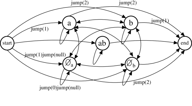
Figure 4: Schematic drawing of the semi-HMM (with some transition probabilities) for the document “a b”

In our case, the state set is large, but well structured. There is a unique initial state $\langle\text{start}\rangle$, a unique final state $\langle\text{end}\rangle$, and a state for each possible document phrase. That is, for a document of length $n$, for all $1\leq i\leq i^{\prime}\leq n$, there is a state that corresponds to the document phrase beginning at position $i$ and ending at position $i^{\prime}$, which we will refer to as $r_{i,i^{\prime}}$. There is also a null state for each document position $r_{\emptyset,i}$. Thus, $S=\{\langle\text{start}\rangle,\langle\text{end}\rangle\}\cup\{r_{i,i^{\prime}}:1\leq i\leq i^{\prime}\leq n\}\cup\{r_{\emptyset,i}:1\leq i\leq n\}$. The output alphabet consists of each word found in $S$, plus the end-of-sentence word $\omega$. We only allow the word $\omega$ to be emitted on a transition to the end state. The transition probabilities are managed by the jump model, and the emission probabilities are managed by the rewrite model.

Consider the document “a b” (the semi-HMM for which is shown in Figure 4) in the case when the corresponding summary is “c d.” Suppose the correct alignment is that “c d” is aligned to “a” and “b” is left unaligned. Then, the path taken through the semi-HMM is $\langle\text{start}\rangle\rightarrow a\rightarrow\langle\text{end}\rangle$. During the transition $\langle\text{start}\rangle\rightarrow a$, “c d” is emitted. During the transition $a\rightarrow\langle\text{end}\rangle$, $\omega$ is emitted.

3.4 Expectation maximization

The alignment task, as described above, is a chicken and egg problem: if we knew the model components (namely, the rewrite and jump tables), we would be able to efficiently find the best alignment. Similarly, if we knew the correct alignments, we would be able to estimate the model components. Unfortunately, we have neither. Expectation maximization is a general technique for learning in such chicken and egg problems [Dempster, Laird, and Rubin,1977, Boyles,1983, Wu,1983]. The basic idea is to make a guess at the alignments, then use this guess to estimate the parameters for the relevant distributions. We can use these re-estimated distributions to make a better guess at the alignments, and then use these (hopefully better) alignments to re-estimate the parameters.

Formally, the EM family of algorithms tightly bound the $\log$ of an expectation of a function by the expectation of $\log$ of that function, through the use of Jensen’s inequality [Jensen,1906]. The tightness of the bound means that when we attempt to estimate the model parameters, we may do so over expected alignments, rather that the true (but unknown) alignments. EM gives formal guarantees of convergence, but is only guaranteed to find local maxima.

3.5 Model inference

$$\alpha_{j}(t) = p\left(\boldsymbol{s}_{1:t-1},\textnormal{doc posn}=j\right)=\sum_{t^{\prime}=0}^{t-1}\sum_{i\in S}\alpha_{i}(t^{\prime}+1)\textrm{jump}(j\textrm{~{}}|\textrm{~{}}i)\textrm{rewrite}(\boldsymbol{s}_{1:t-1}\textrm{~{}}|\textrm{~{}}d_{j})$$

$$\beta_{i}(t) = p\left(\boldsymbol{s}_{t:T}\textrm{~{}}|\textrm{~{}}\textnormal{doc posn}=i\right)=\sum_{t^{\prime}=t}^{T}\sum_{j\in S}\textrm{jump}(j\textrm{~{}}|\textrm{~{}}i)\textrm{rewrite}(\boldsymbol{s}_{t:t^{\prime}}\textrm{~{}}|\textrm{~{}}d_{j})\beta_{j}(t^{\prime}+1)$$

$$\zeta_{j}(t) = \max_{i,t^{\prime}}\zeta_{i}(t^{\prime})\textrm{jump}(j\textrm{~{}}|\textrm{~{}}i)\textrm{rewrite}(\boldsymbol{s}_{t^{\prime}:t-1}\textrm{~{}}|\textrm{~{}}d_{j})$$

$$\tau_{i,j}(t^{\prime},t) = \mathcal{E}\{\textnormal{\# transitions $i\leadsto j$ emitting $s_{t^{\prime}:t}$}\}=\frac{\alpha_{i}(t^{\prime})\textrm{jump}(j\textrm{~{}}|\textrm{~{}}i)\textrm{rewrite}(\boldsymbol{s}_{t^{\prime}:t}\textrm{~{}}|\textrm{~{}}d_{j})\beta_{j}(t+1)}{p\left(\boldsymbol{s}_{1:T}\right)}$$

$$\hat{a}_{i,j} = \frac{\mathcal{E}\{\textnormal{\# transitions $i\leadsto j$}\}}{\mathcal{E}\{\textnormal{\# transitions $i\leadsto?$}\}}=\frac{\sum_{t^{\prime}=1}^{T}\sum_{t=t^{\prime}}^{T}\tau_{i,j}(t^{\prime},t)}{\sum_{t^{\prime}=1}^{T}\sum_{t=t^{\prime}}^{T}\sum_{j^{\prime}\in S}\tau_{i,j^{\prime}}(t^{\prime},t)}$$

$$\hat{b}_{i,j,\boldsymbol{k}} = \frac{\mathcal{E}\{\textnormal{\# transitions $i\leadsto j$ with $\boldsymbol{w}$ observed}\}}{\mathcal{E}\{\textnormal{\# transitions $i\leadsto j$}\}}=\frac{\sum_{t:s_{t:t+|\boldsymbol{k}|-1}=\boldsymbol{k}}\tau_{i,j}(t,t+|\boldsymbol{k}|-1)}{\sum_{t^{\prime}=1}^{T}\sum_{t=t^{\prime}}^{T}\tau_{i,j}(t^{\prime},t)}$$

Figure 5: Summary of inference equations for a semi-Markov model

All the inference techniques utilized in this paper are standard applications of semi-Markov model techniques. The relevant equations are summarized in Figure 5 and described below. In all these equations, the variables $t$ and $t^{\prime}$ range over phrases in the summary (specifically, the phrase $\boldsymbol{s}_{t:t^{\prime}}$), and the variables $i$ and $j$ range over phrases in the document. The interested reader is directed to [Ostendorf, Digalakis, and Kimball,1996] for more details on the generic form of these models and their inference techniques.

The standard, and simplest inference problem in our model is to compute $p(\boldsymbol{s}\textrm{~{}}|\textrm{~{}}\boldsymbol{d})$ by summing over all possible alignments. A naïve implementation of this will take time exponential in the length of the summary. Instead, we are able to employ a variant of the forward algorithm to compute these probabilities recursively. The basic idea is to compute the probability of generating a prefix of the summary and ending up at a particular position in the document (this is known as the forward probability). Since our independence assumptions tell us that it does not matter how we got to this position, we can use this forward probability to compute the probability of taking one more step in the summary. At the end, the desired probability $p(\boldsymbol{s}\textrm{~{}}|\textrm{~{}}\boldsymbol{d})$ is simply the forward probability of reaching the end of the summary and document simultaneously. The forward probabilities are calculated in the “$\alpha$ table” in Figure 5. This equation essentially says that the probability of emitting the first $t-1$ words of the summary and ending at position $j$ in the document can be computed by summing over our previous position ($t^{\prime}$) and previous state ($i$) and multiplying the probability of getting there ($\alpha_{i}(t^{\prime}+1)$) with the probability of moving from there to the current position.

The second standard inference problem is the calculation of the best alignment: the Viterbi alignment. This alignment can be computed in exactly the same fashion as the forward algorithm, with two small changes. First, the forward probabilities implicitly include a sum over all previous states, whereas the Viterbi probabilities replace this with a max operator. Second, in order to recover the actual Viterbi alignment, we keep track of which previous state this max operator chose. This is computed by filling out the $\zeta$ table from Figure 5. This is almost identical to the computation of the forward probabilities, except that instead of summing over all possible $t^{\prime}$ and $i$, we take the maximum over those variables.

The final inference problem is parameter re-estimation. In the case of standard HMMs, this is known as the Baum-Welch or Baum-Eagon or Forward-Backward algorithm [Baum and Petrie,1966, Baum and Eagon,1967]. By introducing “backward” probabilities, analogous to the forward probabilities, we can compute alignment probabilities of suffixes of the summary. The backward table is the “$\beta$ table” in Figure 5, which is analogous to the $\alpha$ table, except that the computation proceeds from the end to the start.

By combining the forward and backward probabilities, we can compute the expected number of times a particular alignment was made (the E-step in the EM framework). Based on these expectations, we can simply sum and normalize to get new parameters (the M-step). The expected transitions are computed according to the $\tau$ table, which makes use of the forward and backward probabilities. Finally, the re-estimated jump probabilities are given by $\hat{a}$ and the re-estimated rewrite probabilities are given by $\hat{b}$, which are essentially relative frequencies of the fractional counts given by the $\tau$s.

The computational complexity for the Viterbi algorithm and for the parameter re-estimation is $\mathcal{O}\left(N^{2}T^{2}\right)$, where $N$ is the length of the summary, and $T$ is the number of states (in our case, $T$ is roughly the length of the document times the maximum phrase length allowed). However, we will typically bound the maximum length of a phrase; otherwise we are unlikely to encounter enough training data to get reasonable estimates of emission probabilities. If we enforce a maximum observation sequence length of $l$, then this drops to $\mathcal{O}\left(N^{2}Tl\right)$. Moreover, if the transition network is sparse, as it is in our case, and the maximum out-degree of any node is $b$, then the complexity drops to $\mathcal{O}\left(NTbl\right)$.

4 Model Parameterization

Beyond the conditional independence assumptions made by the semi-HMM, there are nearly no additional constraints that are imposed on the parameterization (in term of the jump and rewrite distributions) of the model. There is one additional technical requirement involving parameter re-estimation, which essentially says that the expectations calculated during the forward-backward algorithm must be sufficient statistics for the parameters of the jump and rewrite models. This constraint simply requires that whatever information we need to re-estimate their parameters is available to us from the forward-backward algorithm.

4.1 Parameterizing the jump model

Recall that the responsibility of the jump model is to compute probabilities of the form $\textrm{jump}(j^{\prime}\textrm{~{}}|\textrm{~{}}j)$, where $j^{\prime}$ is a new position and $j$ is an old position. We have explored several possible parameterizations of the jump table. The first simply computes a table of likely jump distances (i.e., jump forward 1, jump backward 3, etc.). The second models this distribution as a Gaussian (though, based on Figure 2 this is perhaps not the best model). Both of these models have been explored in the machine translation community. Our third parameterization employs a novel syntax-aware jump model that attempts to take advantage of local syntactic information in computing jumps.

4.1.1 The relative jump model.

 

[]Jump probability decomposition; the source state is either the designated start state, the designated end state, a document phrase position spanning from $i$ to $i^{\prime}$ (denoted $r_{i,i^{\prime}}$) for a null state corresponding to position $i$ (denoted $r_{\emptyset,i}$).

  source target probability $\langle\text{start}\rangle$ $r_{i,i^{\prime}}$ $\textrm{jump}_{\textrm{rel}}(i)$ $r_{i,i^{\prime}}$ $r_{j,j^{\prime}}$ $\textrm{jump}_{\textrm{rel}}(j-i^{\prime})$ $r_{i,j^{\prime}}$ $\langle\text{end}\rangle$ $\textrm{jump}_{\textrm{rel}}(m+1-i^{\prime})$ $\langle\text{start}\rangle$ $r_{\emptyset,i}$ $\textrm{jump}_{\textrm{rel}}(\emptyset)\textrm{jump}_{\textrm{rel}}(i)$ $r_{\emptyset,i}$ $r_{j,j^{\prime}}$ $\textrm{jump}_{\textrm{rel}}(j-i)$ $r_{\emptyset,i}$ $r_{\emptyset,j}$ $\textrm{jump}_{\textrm{rel}}(\emptyset)\textrm{jump}_{\textrm{rel}}(j-i)$ $r_{\emptyset,i}$ $\langle\text{end}\rangle$ $\textrm{jump}_{\textrm{rel}}(m+1-i)$ $r_{i,i^{\prime}}$ $r_{\emptyset,j}$ $\textrm{jump}_{\textrm{rel}}(\emptyset)\textrm{jump}_{\textrm{rel}}(j-i^{\prime})$

In the relative jump model, we keep a table of counts for each possible jump distance, and compute $\textrm{jump}(j^{\prime}\textrm{~{}}|\textrm{~{}}j)=\textrm{jump}_{\textrm{rel}}(j^{\prime}-j)$. Each possible jump type and its associated probability is shown in Table 4.1.1. By these calculations, regardless of document phrase lengths, transitioning forward between two consecutive segments will result in $\textrm{jump}_{\textrm{rel}}(1)$. When transitioning from the start state $p$ to state $r_{i,i^{\prime}}$, the value we use a jump length of $i$. Thus, if we begin at the first word in the document, we incur a transition probability of $j{1}$. There are no transitions into $p$. We additionally remember a specific transition $\textrm{jump}_{\textrm{rel}}(\emptyset)$ for the probability of transitioning to a null state. It is straightforward to estimate these parameters based on the estimations from the forward-backward algorithm. In particular, $\textrm{jump}_{\textrm{rel}}(i)$ is simply the relative frequency of length $i$ jumps and $\textrm{jump}_{\textrm{rel}}(\emptyset)$ is simply the count of jumps that end in a null state to the total number of jumps. The null state “remembers” the position we ended in before we jumped there and so to jump out of a null state, we make a jump based on this previous position.

4.1.2 Gaussian jump model.

The Gaussian jump model attempts to alleviate the sparsity of data problem in the relative jump model by assuming a parametric form to the jumps. In particular, we assume there is a mean jump length $\mu$ and a jump variance $\sigma^{2}$, and then the probability of a jump of length $i$ is given by:

$$i\sim\mathcal{N}\textit{or}(\mu,\sigma^{2})\varpropto\exp\left[\frac{1}{\sigma^{2}}(i-\mu)^{2}\right]$$ (1)

Some care must be taken in employing this model, since the normal distribution is defined over a continuous space. Thus, when we discretize the calculation, the normalizing constant changes slightly from that of a continuous normal distribution. In practice, we normalize by summing over a sufficiently large range of possible $i$s. The parameters $\mu$ and $\sigma^{2}$ are estimated by computing the mean jump length in the expectations and its empirical variance. We model null states identically to the relative jump model.

4.1.3 Syntax-aware jump model.

Both of the previously described jump models are extremely naïve, in that they look only at the distance jumped, and completely ignore what is being jumped over. In the syntax-aware jump model, we wish to enable the model to take advantage of syntactic knowledge in a very weak fashion. This is quite different from the various approaches to incorporating syntactic knowledge into machine translation systems, wherein strong assumptions about the possible syntactic operations are made [Yamada and Knight,2001, Eisner,2003, Gildea,2003].

Figure 6: The syntactic tree for an example document sentence.

To motivate this model, consider the first document sentence shown with its syntactic parse tree in Figure 6. Though it is not always the case, forward jumps of distance more than one are often indicative of skipped words. From the standpoint of the relative jump models, jumping over the four words “tripled it ’s sales” and jumping over the four words “of Apple Macintosh systems” are exactly the same. However, intuitively, we would be much more willing to jump over the latter than the former. The latter phrase is a full syntactic constituent, while the first phrase is just a collection of nearby words. Furthermore, the latter phrase is a prepositional phrase (and prepositional phrases might be more likely dropped than other phrases) while the former phrase includes a verb, a pronoun, a possessive marker and a plain noun.

To formally capture this notion, we parameterize the syntax-aware jump model according to the types of phrases being jumped over. That is, to jump over “tripled it ’s sales” would have probability $\textrm{jump}_{\textrm{syn}}(\textsf{VBD PRP POS NNS})$ while to jump over “of Apple Macintosh systems” would have probability $\textrm{jump}_{\textsf{syn}}(\textsf{PP})$. In order to compute the probabilities for jumps over many components, we factorize so that the first probability becomes $\textrm{jump}_{\textsf{syn}}(\textsf{VBD})\textrm{jump}_{\textsf{syn}}(\textsf{PRP})\textrm{jump}_{\textsf{syn}}(\textsf{POS})\textrm{jump}_{\textsf{syn}}(\textsf{NNS})$. This factorization explicitly encodes our preference for jumping over single units, rather than several syntactically unrelated units.

In order to work with this model, we must first parse the document side of the corpus; we used Charniak’s parser [Charniak,1997]. Given the document parse trees, the re-estimation of the components of this probability distribution is done by simply counting what sorts of phrases are being jumped over. Again, we keep a single parameter $\textrm{jump}_{\textrm{syn}}(\emptyset)$ for jumping to null states. To handle backward jumps, we simply consider a duplication of the tag set, where $\textrm{jump}_{\textrm{syn}}(\textsf{NP-f})$ denotes a forward jump over an NP and $\textrm{jump}_{\textrm{syn}}(\textsf{NP-b})$ denotes a backward jump over an NP.

4.2 Parameterizing the rewrite model

As observed from the human-aligned summaries, a good rewrite model should be able to account for alignments between identical word and phrases, between words that are identical up to stem, and between different words. Intuition (as well as further investigations of the data) also suggest that synonymy is an important factor to take into consideration in a successful rewrite model. We account for each of these four factors in four separate components of the model and then take a linear interpolation of them to produce the final probability:

$$\textrm{rewrite}(\boldsymbol{s}\textrm{~{}}|\textrm{~{}}\boldsymbol{d}) =\lambda_{\textrm{id}}\textrm{rewrite}_{\textrm{id}}(\boldsymbol{s}\textrm{~{}}|\textrm{~{}}\boldsymbol{d})+\lambda_{\textrm{stem}}\textrm{rewrite}_{\textrm{stem}}(\boldsymbol{s}\textrm{~{}}|\textrm{~{}}\boldsymbol{d})$$ (2)

$$+\lambda_{\textrm{wn}}\textrm{rewrite}_{\textrm{wn}}(\boldsymbol{s}\textrm{~{}}|\textrm{~{}}\boldsymbol{d})+\lambda_{\textrm{rw}}\textrm{rewrite}_{\textrm{rw}}(\boldsymbol{s}\textrm{~{}}|\textrm{~{}}\boldsymbol{d})$$ (3)

where the $\lambda$s are constrained to sum to unity. The four rewrite distributions used are: id is a word identity model, which favors alignment of identical words; stem is a model designed to capture the notion that matches at the stem level are often sufficient for alignment (i.e., “walk” and “walked” are likely to be aligned); wn is a rewrite model based on similarity according to WordNet; and wr is the basic rewrite model, similar to a translation table in machine translation. These four models are described in detail below, followed by a description of how to compute their $\lambda$s during EM.

4.2.1 Word identity rewrite model.

The form of the word identity rewrite model is: $\textrm{rewrite}_{\textrm{id}}(\boldsymbol{s}\textrm{~{}}|\textrm{~{}}\boldsymbol{d})=\delta_{\boldsymbol{s}=\boldsymbol{d}}$. That is, the probability is $1$ exactly when $\boldsymbol{s}$ and $\boldsymbol{d}$ are identical, and $0$ when they differ. This model has no parameters.

4.2.2 Stem identity rewrite model.

The form of the stem identity rewrite model is very similar to that of the word identity model:

$$\textrm{rewrite}_{\textrm{stem}}(\boldsymbol{s}\textrm{~{}}|\textrm{~{}}\boldsymbol{d})=\frac{1}{Z_{\boldsymbol{d}}}\delta_{|\boldsymbol{s}|=|\boldsymbol{d}|}\prod_{i=1}^{|\boldsymbol{s}|}\delta_{\textit{stem}(s_{i})=\textit{stem}(d_{i})}$$ (4)

That is, the probability of a phrase $\boldsymbol{s}$ given $\boldsymbol{d}$ is uniform over all phrases $\boldsymbol{s}^{\prime}$ that match $\boldsymbol{d}$ up to stem (and are of the same length, i.e., $|\boldsymbol{s}^{\prime}|=|\boldsymbol{d}|$), and zero otherwise. The normalization constant is computed offline based on a pre-computed vocabulary. This model also has no parameters.

4.2.3 WordNet rewrite model.

In order to account for synonymy, we allow document phrases to be rewritten to semantically “related” summary phrases. To compute the value for $\textrm{rewrite}_{\textrm{wn}}(\boldsymbol{s}\textrm{~{}}|\textrm{~{}}\boldsymbol{d})$ we first require that both $\boldsymbol{s}$ and $\boldsymbol{d}$ can be found in WordNet. If either cannot be found, then the probability is zero. If they both can be found, then the graph distance between their first senses is computed (we traverse the hypernymy tree up until they meet). If the two paths do not meet, then the probability is again taken to be zero. We place an exponential model on the hypernym tree-based distance:

$$\textrm{rewrite}_{\textrm{wn}}(\boldsymbol{s}\textrm{~{}}|\textrm{~{}}\boldsymbol{d})=\frac{1}{Z_{\boldsymbol{d}}}\exp\left[-\eta\textit{dist}(\boldsymbol{s},\boldsymbol{d})\right]$$ (5)

Here, dist is calculated distance, taken to be $+\infty$ whenever either of the failure conditions is met. The single parameter of this model is $\eta$, which is computed according to the maximum likelihood criterion from the expectations during training. The normalization constant $Z_{\boldsymbol{d}}$ is calculated by summing over the exponential distribution for all $\boldsymbol{s}^{\prime}$ that occur on the summary side of our corpus.

4.2.4 Lexical rewrite model.

The lexical rewrite model is the “catch all” model to handle the cases not handled by the above models. It is analogous to a translation-table (t-table) in statistical machine translation (we will continue to use this terminology for the remainder of the article), and simply computes a matrix of (fractional) counts corresponding to all possible phrase pairs. Upon normalization, this matrix gives the rewrite distribution.

4.2.5 Estimation of the weight parameters.

In order to weight the four models, we need to estimate values for the $\lambda$ components. This computation can be performed inside of the EM iterations, by considering, for each rewritten pair, its expectation of belonging to each of the models. We use these expectations to maximize the likelihood with respect to the $\lambda$s and then normalize them so they sum to one.

4.3 Model priors

In the standard HMM case, the learning task is simply one of parameter estimation, wherein the maximum likelihood criterion under which the parameters are typically trained performs well. However, in our model, we are, in a sense, simultaneously estimating parameters and selecting a model: the model selection is taking place at the level of deciding how to segment the observed summary. Unfortunately, in such model selection problems, likelihood increases monotonically with model complexity. Thus, EM will find for us the most complex model; in our case, this will correspond to a model in which the entire summary is produced at once, and no generalization will be possible.

This suggests that a criterion other than maximum likelihood (ML) is more appropriate. We advocate the maximum a posteriori (MAP) criterion in this case. While ML optimizes the probability of the data given the parameters (the likelihood), MAP optimizes the product of the probability of the parameters with the likelihood (the unnormalized posterior). The difficulty in our model that makes ML estimation perform poorly is centered in the lexical rewrite model. Under ML estimation, we will simply insert an entry in the t-table for the entire summary for some uncommon or unique document word and be done. However, a priori we do not believe that such a parameter is likely. The question then becomes how to express this in a way that inference remains tractable.

From a statistical point of view, the t-table is nothing but a large multinomial model (technically, one multinomial for each possible document phrase). Under a multinomial distribution with parameter $\boldsymbol{\theta}$ with $J$-many components (with all $\theta_{j}$ positive and summing to one), the probability of an observation $\boldsymbol{x}$ is given by (here, we consider $\boldsymbol{x}$ to be a vector of length $J$ in which all components are zero except for one, corresponding to the actual observation): $p\left(\boldsymbol{x}\textrm{~{}}|\textrm{~{}}\boldsymbol{\theta}\right)=\prod_{j=1}^{J}\theta_{j}^{x_{j}}$.

This distribution belongs to the exponential family and therefore has a natural conjugate distribution. Informally, two distributions are conjugate if you can multiply them together and get the original distribution back. In the case of the multinomial, the conjugate distribution is the Dirichlet distribution. A Dirichlet distribution is parameterized by a vector $\boldsymbol{\alpha}$ of length $J$ with $\alpha_{j}\geq 0$, but not necessarily summing to one. The Dirichlet distribution can be used as a prior distribution over multinomial parameters and has density: $p\left(\boldsymbol{\theta}\textrm{~{}}|\textrm{~{}}\boldsymbol{\alpha}\right)=\frac{\Gamma\left(\sum_{j=1}^{J}\alpha_{j}\right)}{\prod_{j=1}^{J}\Gamma(\alpha_{j})}\prod_{j=1}^{J}\theta_{j}^{\alpha_{j}-1}$. The fraction before the product is simply a normalization term that ensures that the integral over all possible $\boldsymbol{\theta}$ integrates to one.

The Dirichlet is conjugate to the multinomial because when we compute the posterior of $\boldsymbol{\theta}$ given $\boldsymbol{\alpha}$ and $\boldsymbol{x}$, we arrive back at a Dirichlet distribution: $p\left(\boldsymbol{\theta}\textrm{~{}}|\textrm{~{}}\boldsymbol{x},\boldsymbol{\alpha}\right)\varpropto p\left(\boldsymbol{x}\textrm{~{}}|\textrm{~{}}\boldsymbol{\theta}\right)p\left(\boldsymbol{\theta}\textrm{~{}}|\textrm{~{}}\boldsymbol{\alpha}\right)\varpropto\prod_{j=1}^{J}\theta_{j}^{x_{j}+\alpha_{j}-1}$. This distribution has the same density as the original model, but a “fake count” of $\alpha_{j}-1$ has been added to component $j$. This means that if we are able to express our prior beliefs about the multinomial parameters found in the t-table in the form of a Dirichlet distribution, the computation of the MAP solution can be performed exactly as described before, but with the appropriate fake counts added to the observed variables (in our case, the observed variables are the alignments between a document phrase and a summary phrase). The application of Dirichlet priors to standard HMMs has previously been considered in signal processing [Gauvain and Lee,1994]. These fake counts act as a smoothing parameter, similar to Laplace smoothing (Laplace smoothing is the special case where $\alpha_{j}=2$ for all $j$).

In our case, we believe that singleton rewrites are worth $2$ fake counts, that lexical identity rewrites are worth $4$ fake counts and that stem identity rewrites are worth $3$ fake counts. Indeed, since a singleton alignment between identical words satisfies all of these criterion, it will receive a fake count of $9$. The selection of these counts is intuitive, but, clearly, arbitrary. However, this selection was not “tuned” to the data to get better performance. As we will discuss later, inference in this model over the sizes of documents and summaries we consider is quite computationally expensive. We appropriately specified this prior according to our prior beliefs, and left the rest to the inference mechanism.

4.4 Parameter initialization

We initialize all the parameters uniformly, but in the case of the rewrite parameters, since there is a prior on them, they are effectively initialized to the maximum likelihood solution under their prior.

5 Experimental Results

The experiments we perform are on the same Ziff-Davis corpus described in the introduction. In order to judge the quality of the alignments produced, we compare them against the gold standard references annotated by the humans. The standard precision and recall metrics used in information retrieval are modified slightly to deal with the “sure” and “possible” alignments created during the annotation process. Given the set $S$ of sure alignments, the set $S\subseteq P$ of possible alignments and a set $A$ of hypothesized alignments we compute the precision as $|A\cap P|/|A|$ and the recall as $|A\cap S|/|S|$.

One problem with these definitions is that phrase-based models are fond of making phrases. That is, when given an abstract containing “the man” and a document also containing “the man,” a human will align “the” to “the” and “man” to “man.” However, a phrase-based model will almost always prefer to align the entire phrase “the man” to “the man.” This is because it results in fewer probabilities being multiplied together.

To compensate for this, we define soft precision (SoftP in the tables) by counting alignments where “a b” is aligned to “a b” the same as ones in which “a” is aligned to “a” and “b” is aligned to “b.” Note, however, that this is not the same as “a” aligned to “a b” and “b” aligned to “b”. This latter alignment will, of course, incur a precision error. The soft precision metric induces a new, soft F-Score, labeled SoftF.

Often, even humans find it difficult to align function words and punctuation. A list of $58$ function words and punctuation marks which appeared in the corpus (henceforth called the ignore-list) was assembled. We computed precision and recall scores both on all words, as well as on all words that do not appear in the ignore-list.

5.1 Systems compared

Overall, we compare various parameter settings of our model against three other systems. First, we compare against two alignment models developed in the context of machine translation. Second, we compare against the Cut and Paste model developed in the context of “summary decomposition” by Jing [Jing,2002]. Each of these systems will be discussed in more detail shortly. However, the machine translation alignment models assume sentence pairs as input. Moreover, even though the semi-Markov model is based on efficient dynamic programming techniques, it is still too inefficient to run on very long $\langle$document, abstract$\rangle$ pairs.

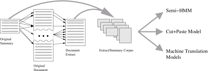
Figure 7: Pictorial representation of the conversion of the $\langle$document, abstract$\rangle$ corpus to an $\langle$extract, abstract$\rangle$ corpus.

To alleviate both of these problems, we preprocess our $\langle$document, abstract$\rangle$ corpus down to an $\langle$extract, abstract$\rangle$ corpus, and then subsequently apply our models to this smaller corpus (see Figure 7). In our data, doing so does not introduce significant noise. To generate the extracts, we paired each abstract sentence with three sentences from the corresponding document, selected using the techniques described by Marcu [Marcu,1999]. In an informal evaluation, $20$ such pairs were randomly extracted and evaluated by a human. Each pair was ranked as $0$ (document sentences contain little-to-none of the information in the abstract sentence), $1$ (document sentences contain some of the information in the abstract sentence) or $2$ (document sentences contain all of the information). Of the twenty random examples, none were labeled as $0$; five were labeled as $1$; and $15$ were labeled as $2$, giving a mean rating of $1.75$. We refer to the resulting corpus as the $\langle$extract, abstract$\rangle$ corpus, statistics for which are shown in Table 5.1. Finally, for fair comparison, we also run the Cut and Paste model only on the extracts.

 

[]Ziff-Davis extract corpus statistics

  Abstracts Extracts Documents Documents $2033$ $2033$ Sentences $13k$ $41k$ $82k$ Words $261k$ $1m$ $2.5m$ Unique words $14k$ $26k$ $42k$ $29k$ Sentences/Doc $6.28$ $21.51$ $40.83$ Words/Doc $128.52$ $510.99$ $1229.71$ Words/Sent $20.47$ $23.77$ $28.36$

5.1.1 Machine translation models.

We compare against several competing systems, the first of which is based on the original IBM Model 4 for machine translation [Brown et al.,1993] and the HMM machine translation alignment model [Vogel, Ney, and Tillmann,1996] as implemented in the GIZA++ package [Och and Ney,2003]. We modified the code slightly to allow for longer inputs and higher fertilities, but otherwise made no changes. In all of these setups, 5 iterations of Model 1 were run, followed by 5 iterations of the HMM model. For Model 4, 5 iterations of Model 4 were subsequently run.

In our model, the distinction between the “summary” and the “document” is clear, but when using a model from machine translation, it is unclear which of the summary and the document should be considered the source language and which should be considered the target language. By making the summary the source language, we are effectively requiring that the fertility of each summary word be very high, or that many words are null generated (since we must generate all of the document). By making the document the source language, we are forcing the model to make most document words have zero fertility. We have performed experiments in both directions, but the latter (document as source) performs better in general.

In order to “seed” the machine translation model so that it knows that word identity is a good solution, we appended our corpus with “sentence pairs” consisting of one “source” word and one “target” word, which were identical. This is common practice in the machine translation community when one wishes to cheaply encode knowledge from a dictionary into the alignment model.

5.1.2 Cut and Paste model.

We also tested alignments using the Cut and Paste summary decomposition method [Jing,2002], based on a non-trainable HMM. Briefly, the Cut and Paste HMM searches for long contiguous blocks of words in the document and abstract that are identical (up to stem). The longest such sequences are aligned. By fixing a length cutoff of $n$ and ignoring sequences of length less than $n$, one can arbitrarily increase the precision of this method. We found that $n=2$ yields the best balance between precision and recall (and the highest F-measure). On this task, this model drastically outperforms the machine translation models.

5.1.3 The semi-Markov model.

While the semi-HMM is based on a dynamic programming algorithm, the effective search space in this model is enormous, even for moderately sized $\langle$document, abstract$\rangle$ pairs. The semi-HMM system was then trained on this $\langle$extract, abstract$\rangle$ corpus. We also restrict the state-space with a beam, sized at $50\%$ of the unrestricted state-space. With this configuration, we run ten iterations of the forward-backward algorithm. The entire computation time takes approximately 8 days on a 128 node cluster computer.

We compare three settings of the semi-HMM. The first, “semi-HMM-relative” uses the relative movement jump table; the second, “semi-HMM-Gaussian” uses the Gaussian parameterized jump table; the third, “semi-HMM-syntax” uses the syntax-based jump model.

5.2 Evaluation results

 

[]Results on the Ziff-Davis corpus

  All Words Non-Stop Words System SoftP Recall SoftF SoftP Recall SoftF Human₁ 0.727 0.746 0.736 0.751 0.801 0.775 Human₂ 0.680 0.695 0.687 0.730 0.722 0.726 HMM (Sum=Src) 0.120 0.260 0.164 0.139 0.282 0.186 Model 4 (Sum=Src) 0.117 0.260 0.161 0.135 0.283 0.183 HMM (Doc=Src) 0.295 0.250 0.271 0.336 0.267 0.298 Model 4 (Doc=Src) 0.280 0.247 0.262 0.327 0.268 0.295 Cut & Paste 0.349 0.379 0.363 0.431 0.385 0.407 semi-HMM-relative 0.456 0.686 0.548 0.512 0.706 0.593 semi-HMM-Gaussian 0.328 0.573 0.417 0.401 0.588 0.477 semi-HMM-syntax 0.504 0.701 0.586 0.522 0.712 0.606

The results, in terms of precision, recall and f-score are shown in Table 5.2. The first three columns are when these three statistics are computed over all words. The next three columns are when these statistics are only computed over words that do not appear in our “ignore list” of 58 stop words. Under the methodology for combining the two human annotations by taking the union, either of the human scores would achieve a precision and recall of $1.0$. To give a sense of how well humans actually perform on this task, we compare each human against the other.

As we can see from Table 5.2, none of the machine translation models is well suited to this task, achieving, at best, an F-score of $0.298$. The “flipped” models, in which the document sentences are the “source” language and the abstract sentences are the “target” language perform significantly better (comparatively). Since the MT models are not symmetric, going the bad way requires that many document words have zero fertility, which is difficult for these models to cope with.

The Cut & Paste method performs significantly better, which is to be expected, since it is designed specifically for summarization. As one would expect, this method achieves higher precision than recall, though not by very much. The fact that the Cut & Paste model performs so well, compared to the MT models, which are able to learn non-identity correspondences, suggests that any successful model should be able to take advantage of both, as ours does.

Our methods significantly outperform both the IBM models and the Cut & Paste method, achieving a precision of $0.522$ and a recall of $0.712$, yielding an overall F-score of $0.606$ when stop words are not considered. This is still below the human-against-human f-score of $0.775$ (especially considering that the true human-against-human scores are $1.0$), but significantly better than any of the other models.

Among the three settings of our jump table, the syntax-based model performs best, followed by the relative jump model, with the Gaussian model coming in worst (though still better than any other approach). Inspecting Figure 2, the fact that the Gaussian model does not perform well is not surprising: the data shown there is very non-Gaussian. A double-exponential model might be a better fit, but it is unlikely that such a model will outperform the syntax based model, so we did not perform this experiment.

5.3 Error analysis

Example 1:

   

Example 2:

Figure 8: Erroneous alignments are in bold. (Top) Example of an error made by our model (from file ZF207-585-936). “From DOS” should be null generated, but the model has erroneously aligned it to an identical phrase that appeared 11 sentences earlier in the document. (Bottom) Error (from ZF207-772-628); “The DMP 300” should be aligned to “the printer” but is instead aligned to a far-away occurrence of “The DMP 300.”

The first mistake frequently made by our model is to not align summary words to null. In effect, this means that our model of null-generated summary words is lacking. An example of this error is shown in Example 1 in Figure 8. In this example, the model has erroneously aligned “from DOS” in the abstract to “from DOS” in the document (the error is shown in bold). This alignment is wrong because the context of “from DOS” in the document is completely different from the context it appears in in the summary. However, the identity rewrite model has overwhelmed the locality model and forced this incorrect alignment. To measure the frequency of such errors, we have post-processed our system’s alignments so that whenever a human alignment contains a null-generated summary word, our model also predicts that this word is null-generated. Doing so will not change our system’s recall, but it can improve the precision. Indeed, in the case of the relative jump model, the precision jumps from $0.456$ to $0.523$ (f-score increases from $0.548$ to $0.594$) in the case of all words and from $0.512$ to $0.559$ (f-score increases from $0.593$ to $0.624$). This corresponds to a relative improvement of roughly $8\%$ f-score. Increases in score for the syntax-based model are roughly the same.

 

[]10 example phrase alignments from the hand-annotated corpus; last column indicates whether the semi-HMM correctly aligned this phrase.

  Summary Phrase True Phrase Aligned Phrase Class to port can port to port incorrect OS - 2 the OS / 2 OS / 2 partial will use will be using will using partial word processing programs word processors word processing incorrect consists of also includes null of partial will test will also have to test will test partial the potential buyer many users the buyers incorrect The new software Crosstalk for Windows new software incorrect are generally powered by run on null incorrect Oracle Corp. the software publisher Oracle Corp. incorrect

The second mistake our model frequently makes is to trust the identity rewrite model too strongly. This problem has to do either with synonyms that do not appear frequently enough for the system to learn reliable rewrite probabilities, or with coreference issues, in which the system chooses to align, for instance, “Microsoft” to “Microsoft,” rather than “Microsoft” to “the company,” as might be correct in context. As suggested by this example, this problem is typically manifested in the context of coreferential noun phrases. It is difficult to perform a similar analysis of this problem as for the aforementioned problem (to achieve an upper bound on performance), but we can provide some evidence. As mentioned before, in the human alignments, roughly $51\%$ of all aligned phrases are lexically identical. In the alignments produced by our model (on the same documents), this number is $69\%$. In the case of stem identity, the hand align data suggests that stem identity should hold in $67\%$ of the cases; in our alignments, this number was $81\%$. An example of this sort of error is shown in Example 2 in Figure 8. Here, the model has aligned “The DMP 300” in the abstract to “The DMP 300” in the document, while it should have been aligned to “the printer” due to locality constraints (note that the model also misses the (produces $\leftrightarrow$ producing) alignment, likely as a side-effect of it making the error depicted in bold).

In Table 5.3, we have shown examples of common errors made by our system (these were randomly selected from a much longer list of errors). These examples are shown out of their contexts, but in most cases, the error is clear even so. In the first column, we show the summary phrase in question. In the second column, we show the document phrase do which it should be aligned, and in the third column, we show the document phrase that our model aligned it to (or “null”). In the right column, we classify the model’s alignment as “incorrect” or “partially correct.”

The errors shown in Table 5.3 show several weaknesses of the model. For instance, in the first example, it aligns “to port” with “to port,” which seems correct without context, but the chosen occurrence of “to port” in the document is in the discussion of a completely different porting process than that referred to in the summary (and is several sentences away). The seventh and tenth examples (“The new software” and “Oracle Corp.” respectively) show instances of the coreference error that occurs commonly.

6 Conclusion and Discussion

Currently, summarization systems are limited to either using hand-annotated data, or using weak alignment models at the granularity of sentences, which serve as suitable training data only for sentence extraction systems. To train more advanced extraction systems, such as those used in document compression models or in next-generation abstraction models, we need to better understand the lexical correspondences between documents and their human written abstracts. Our work is motivated by the desire to leverage the vast number of $\langle$document, abstract$\rangle$ pairs that are freely available on the internet and in other collections, and to create word- and phrase-aligned $\langle$document, abstract$\rangle$ corpora automatically.

This paper presents a statistical model for learning such alignments in a completely unsupervised manner. The model is based on an extension of a hidden Markov model, in which multiple emissions are made in the course of one transition. We have described efficient algorithms in this framework, all based on dynamic programming. Using this framework, we have experimented with complex models of movement and lexical correspondences. Unlike the approaches used in machine translation, where only very simple models are used, we have shown how to efficiently and effectively leverage such disparate knowledge sources and WordNet, syntax trees and identity models.

We have empirically demonstrated that our model is able to learn the complex structure of $\langle$document, abstract$\rangle$ pairs. Our system outperforms competing approaches, including the standard machine translation alignment models [Brown et al.,1993, Vogel, Ney, and Tillmann,1996] and the state of the art Cut & Paste summary alignment technique [Jing,2002].

We have analyzed two sources of error in our model, including issues of null-generated summary words and lexical identity. Within the model itself, we have already suggested two major sources of error in our alignment procedure. Clearly more work needs to be done to fix these problems. One approach that we believe will be particularly fruitful would be to add a fifth model to the linearly interpolated rewrite model based on lists of synonyms automatically extracted from large corpora. Additionally, investigating the possibility of including some sort of weak coreference knowledge into the model might serve to help with the second class of errors made by the model.

One obvious aspect of our method that may reduce its general usefulness is the computation time. In fact, we found that despite the efficient dynamic programming algorithms available for this model, the state space and output alphabet are simply so large and complex that we were forced to first map documents down to extracts before we could process them (and even so, computation took roughly 1000 processor hours). Though we have not done so in this work, we do believe that there is room for improvement computationally, as well. One obvious first approach would be to run a simpler model for the first iteration (for example, Model 1 from machine translation [Brown et al.,1993], which tends to be very “recall oriented”) and use this to see subsequent iterations of the more complex model. By doing so, one could recreate the extracts at each iteration using the previous iteration’s parameters to make better and shorter extracts. Similarly, one might only allow summary words to align to words found in their corresponding extract sentences, which would serve to significantly speed up training and, combined with the parameterized extracts, might not hurt performance. A final option, but one that we do not advocate, would be to give up on phrases and train the model in a word-to-word fashion. This could be coupled with heuristic phrasal creation as is done in machine translation [Och and Ney,2000], but by doing so, one completely loses the probabilistic interpretation that makes this model so pleasing.

Aside from computational considerations, the most obvious future effort along the vein of this model is to incorporate it into a full document summarization system. Since this can be done in many ways, including training extraction systems, compression systems, headline generation systems and even extraction systems, we leave this to future work so that we could focus specifically on the alignment task in this paper. Nevertheless, the true usefulness of this model will be borne out by its application to true summarization tasks.

References

- [Aydin, Altunbasak, and Borodovsky,2004] Aydin, Zafer, Yucel Altunbasak, and Mark Borodovsky. 2004. Protein secondary structure prediction with semi-Markov HMMs. In Proceedings of the IEEE International Conference on Acoustics, Speech and Signal Processing (ICASSP), May.
- [Banko, Mittal, and Witbrock,2000] Banko, Michele, Vibhu Mittal, and Michael Witbrock. 2000. Headline generation based on statistical translation. In Proceedings of the Conference of the Association for Computational Linguistics (ACL), pages 318–325, Hong Kong, October 1–8.
- [Barzilay and Elhadad,2003] Barzilay, Regina and Noemie Elhadad. 2003. Sentence alignment for monolingual comparable corpora. In Proceedings of the Conference on Empirical Methods in Natural Language Processing (EMNLP), pages 25–32.
- [Baum and Eagon,1967] Baum, Leonard E. and J.E. Eagon. 1967. An inequality with applications to statistical estimation for probabilistic functions of Markov processes and to a model of ecology. Bulletins of the American Mathematical Society, 73:360–363.
- [Baum and Petrie,1966] Baum, Leonard E. and Ted Petrie. 1966. Statistical inference for probabilistic functions of finite state Markov chains. Annals of Mathematical Statistics, 37:1554–1563.
- [Berger and Mittal,2000] Berger, Adam and Vibhu Mittal. 2000. Query-relevant summarization using FAQs. In Proceedings of the Conference of the Association for Computational Linguistics (ACL), pages 294–301, Hong Kong, October 1–8.
- [Boyles,1983] Boyles, Russell A. 1983. On the convergence of the EM algorithm. Journal of the Royal Statistical Society, B(44):47–50.
- [Brown et al.,1993] Brown, Peter F., Stephen A. Della Pietra, Vincent J. Della Pietra, and Robert L. Mercer. 1993. The mathematics of statistical machine translation: Parameter estimation. Computational Linguistics, 19(2):263–311.
- [Carletta,1995] Carletta, Jean. 1995. Assessing agreement on classification tasks: the kappa statistic. Computational Linguistics, 22(2):249–254.
- [Carroll et al.,1998] Carroll, John, Guido Minnen, Yvonne Canning, Siobhan Devlin, and John Tait. 1998. Practical simplification of English newspaper text to assist aphasic readers. In Proceedings of the AAAI-98 Workshop on Integrating Artificial Intelligence and Assistive Technology.
- [Chandrasekar, Doran, and Bangalore,1996] Chandrasekar, Raman, Christy Doran, and Srinivas Bangalore. 1996. Motivations and methods for text simplification. In Proceedings of the International Conference on Computational Linguistics (COLING), pages 1041–1044, Copenhagen, Denmark.
- [Charniak,1997] Charniak, Eugene. 1997. Statistical parsing with a context-free grammar and word statistics. In Proceedings of the Fourteenth National Conference on Artificial Intelligence (AAAI’97), pages 598–603, Providence, Rhode Island, July 27–31.
- [Daumé III and Marcu,2002] Daumé III, Hal and Daniel Marcu. 2002. A noisy-channel model for document compression. In Proceedings of the Conference of the Association for Computational Linguistics (ACL), pages 449–456.
- [Daumé III and Marcu,2004] Daumé III, Hal and Daniel Marcu. 2004. A tree-position kernel for document compression. In Proceedings of the Fourth Document Understanding Conference (DUC 2004), Boston, MA, May 6 – 7.
- [Dempster, Laird, and Rubin,1977] Dempster, A.P., N.M. Laird, and D.B. Rubin. 1977. Maximum likelihood from incomplete data via the EM algorithm. Journal of the Royal Statistical Society, B39.
- [Edmundson,1969] Edmundson, H.P. 1969. New methods in automatic abstracting. Journal of the Association for Computing Machinery, 16(2):264–285. Reprinted in Advances in Automatic Text Summarization, I. Mani and M.T. Maybury, (eds.).
- [Eisner,2003] Eisner, Jason. 2003. Learning non-isomorphic tree mappings for machine translation. In Proceedings of the Conference of the Association for Computational Linguistics (ACL).
- [Ferguson,1980] Ferguson, Jack D. 1980. Variable duration models for speech. In Proceedings of the Symposium on the Application of Hidden Markov Models to Text and Speech, pages 143–179, October.
- [Gales and Young,1993] Gales, Mark J.F. and Steve J. Young. 1993. The theory of segmental hidden Markov models. Technical report, Cambridge University Engineering Department.
- [Gauvain and Lee,1994] Gauvain, Jean-Luc and Chin-Hui Lee. 1994. Maximum a-posteriori estimation for multivariate gaussian mixture observations of Markov chains. IEEE Transactions Speech and Audio Processing, 2:291–298.
- [Ge and Smyth,2000] Ge, Xianping and Padhraic Smyth. 2000. Segmental semi-Markov models for change-point detection with applications to semiconductor manufacturing. Technical report, University of California at Irvine, March.
- [Gildea,2003] Gildea, Daniel. 2003. Loosely tree-based alignment for machine translation. In Proceedings of the Conference of the Association for Computational Linguistics (ACL), pages 80–87.
- [Grefenstette,1998] Grefenstette, Gregory. 1998. Producing intelligent telegraphic text reduction to provide an audio scanning service for the blind. In Working Notes of the AAAI Spring Symposium on Intelligent Text Summarization, pages 111–118, Stanford University, CA, March 23-25.
- [Jensen,1906] Jensen, J.L.W.V. 1906. Sur les fonctions convexes et les inégalités entre les valeurs moyennes. Acta Mathematica, 30:175–193.
- [Jing,2000] Jing, Hongyan. 2000. Sentence reduction for automatic text summarization. In Proceedings of the Conference of the North American Chapter of the Association for Computational Linguistics (NAACL), pages 310–315, Seattle, WA.
- [Jing,2002] Jing, Hongyan. 2002. Using hidden markov modeling to decompose human-written summaries. Computational Linguistics, 28(4):527 – 544, December.
- [Knight and Marcu,2002] Knight, Kevin and Daniel Marcu. 2002. Summarization beyond sentence extraction: A probabilistic approach to sentence compression. Artificial Intelligence, 139(1).
- [Kupiec, Pedersen, and Chen,1995] Kupiec, Julian, Jan O. Pedersen, and Francine Chen. 1995. A trainable document summarizer. In Research and Development in Information Retrieval, pages 68–73.
- [Luhn,1956] Luhn, H.P. 1956. The automatic creation of literature abstracts. In Inderjeet Mani and Mark Maybury, editors, Advances in Automatic Text Summarization. The MIT Press, Cambridge, MA, pages 58–63.
- [Mahesh,1997] Mahesh, Kavi. 1997. Hypertext summary extraction for fast document browsing. In Proceedings of the AAAI Spring Symposium on Natural Language Processing for the World Wide Web, pages 95–103.
- [Mani,2001] Mani, Inderjeet. 2001. Automatic Summarization, volume 3 of Natural Language Processing. John Benjamins Publishing Company, Amsterdam/Philadelphia.
- [Mani and Maybury,1999] Mani, Inderjeet and Mark Maybury, editors. 1999. Advances in Automatic Text Summarization. The MIT Press, Cambridge, MA.
- [Marcu,1999] Marcu, Daniel. 1999. The automatic construction of large-scale corpora for summarization research. In Proceedings of the 22nd Conference on Research and Development in Information Retrieval (SIGIR–99), pages 137–144, Berkeley, CA, August 15–19.
- [Marcu,2000] Marcu, Daniel. 2000. The Theory and Practice of Discourse Parsing and Summarization. The MIT Press, Cambridge, Massachusetts.
- [Mitchell, Jamieson, and Harper,1995] Mitchell, Carl D., Leah H. Jamieson, and Mary P. Harper. 1995. On the complexity of explicit duration HMMs. IEEE Transactions on Speech and Audio Processing, 3(3), May.
- [Och and Ney,2000] Och, Franz Josef and Hermann Ney. 2000. Improved statistical alignment models. In Proceedings of the Conference of the Association for Computational Linguistics (ACL), pages 440–447, October.
- [Och and Ney,2003] Och, Franz Josef and Hermann Ney. 2003. A systematic comparison of various statistical alignment models. Computational Linguistics, 29(1):19–51.
- [Ostendorf, Digalakis, and Kimball,1996] Ostendorf, Mari, Vassilis Digalakis, and Owen Kimball. 1996. From HMMs to segment models: A unified view of stochastic modeling for speech recognition. IEEE Transactions on Speech and Audio Processing, 4(5):360–378, September.
- [Quirk, Brockett, and Dolan,2004] Quirk, Chris, Chris Brockett, and William Dolan. 2004. Monolingual machine translation for paraphrase generation. In Proceedings of the Conference on Empirical Methods in Natural Language Processing (EMNLP), pages 142–149, Barcelona, Spain.
- [Schwartz, Zajic, and Dorr,2002] Schwartz, Richard, David Zajic, and Bonnie Dorr. 2002. Automatic headline generation for newspaper stories. In Proceedings of the Document Understanding Conference (DUC), pages 78–85.
- [Smyth, Heckerman, and Jordan,1997] Smyth, Padhraic, David Heckerman, and Michael I. Jordan. 1997. Probabilistic independence networks for hidden Markov probability models. Neural Computation, 9(2):227–269.
- [Teufel and Moens,1997] Teufel, Simone and Mark Moens. 1997. Sentence extraction as a classification task. In In ACL/EACL-97 Workshop on Intelligent and Scalable Text Summarization, pages 58–65.
- [Vogel, Ney, and Tillmann,1996] Vogel, Stephan, Hermann Ney, and Christoph Tillmann. 1996. HMM-based word alignment in statistical translation. In Proceedings of the International Conference on Computational Linguistics (COLING), pages 836–841.
- [Wu,1983] Wu, Jeff C.F. 1983. On the convergence properties of the EM algorithm. The Annals of Statistics, 11:95–103.
- [Yamada and Knight,2001] Yamada, Kenji and Kevin Knight. 2001. A syntax-based statistical translation model. In Proceedings of the Conference of the Association for Computational Linguistics (ACL), pages 523–530.
- [Zajic, Dorr, and Schwartz,2004] Zajic, David, Bonnie Dorr, and Richard Schwartz. 2004. BBN/UMD at DUC-2004: Topiary. In Proceedings of the Fourth Document Understanding Conference (DUC 2004), Boston, MA, May 6 – 7.