Tensors and n-d Arrays:
A Mathematics of Arrays (MoA), $\psi$-Calculus and the Composition of Tensor and Array Operations

Abstract

The Kronecker product is a key algorithm and is ubiquitous across the physical, biological, and computation social sciences. Thus considerations of optimal implementation are important. The need to have high performance and computational reproducibility is paramount. Moreover, due to the need to compose multiple Kronecker products, issues related to data structures, layout and indexing algebra require a new look at an old problem. This paper discusses the outer product/tensor product and a special case of the tensor product: the Kronecker product, along with optimal implementation when composed, and mapped to complex processor/memory hierarchies. We discuss how the use of A Mathematics of Arrays (MoA), and the $\psi$ - Calculus, (a calculus of indexing with shapes), provides optimal, verifiable, reproducible, scalable, and portable implementations of both hardware and software [6, 9, 7, 8].

1 Introduction

The purpose of this report is to discuss the outer product/tensor product and a special case of the tensor product: the Kronecker product, as well as algorithms, their origin, and optimal implementation when composed, and mapped to complex processor/memory hierarchies [13, 2, 1, 5, 12, 3, 4, 11, 10]. We discuss how the use of A Mathematics of Arrays (MoA), and the $\psi$ - Calculus, (a calculus of indexing with shapes), provides optimal, verifiable, reproducible, scalable, and portable implementations of both hardware and software [6, 9, 7, 8]. This is due to the fact that we are using normal forms composed of multi-linear operations on Cartesian coordinates which are transformed into simple abstract machines: starts, stops, strides, count, up and down the processor/memory hierarchy. Before turning the the discussion at hand we invite the reader to consult the appendix for motivational background illustrating how tensor/Kronecker products and diadics arise naturally in applied problems in physics and engineering.

A key notion of the present work is how the MoA outer product can be formulated as the Kronecker product, a special case of the Tensor product. We will show that the use of the MoA outer product is superior to the traditional approach when one is concerned with efficient implementations of multiple Kronecker products. The MoA outer product is a general operation on two arrays of any shape or dimension and applies any scalar operation, not just the product ($*$) on these two arrays (i.e. $+$, $-$, $/$, etc. are valid operations). For now, we focus on the relationship to the Kronecker product between two matrices of arbitrary size resulting in a block matrix. Let’s begin with an example where:

$$A=\left[\begin{array}[]{cc}1&2\\ 3&4\\ \end{array}\right],\mbox{ and }B=\left[\begin{array}[]{cccc}5&6&7&8\\ 9&10&11&12\\ 13&14&15&16\end{array}\right],$$

the operation:

$$A\bigotimes B,$$

is defined by the operation in Fig. 1.

$$\left[\begin{array}[]{cc}1&2\\ 3&4\\ \end{array}\right]\bigotimes\left[\begin{array}[]{cccc}5&6&7&8\\ 9&10&11&12\\ 13&14&15&16\end{array}\right]=$$

$$\left[\begin{array}[]{llllllll}1\times 5&1\times 6&1\times 7&1\times 8&2\times 5&2\times 6&2\times 7&2\times 8\\ 1\times 9&1\times 10&1\times 11&1\times 12&2\times 9&2\times 10&2\times 11&2\times 12\\ 1\times 13&1\times 14&1\times 15&1\times 16&2\times 13&2\times 14&2\times 15&2\times 16\\ 3\times 5&3\times 6&3\times 7&3\times 8&4\times 5&4\times 6&4\times 7&4\times 8\\ 3\times 9&3\times 10&3\times 11&3\times 12&4\times 9&4\times 10&4\times 11&4\times 12\\ 3\times 13&3\times 14&3\times 15&3\times 16&4\times 13&4\times 14&4\times 15&4\times 16\\ \end{array}\right]$$

Figure 1: Kronecker product of A and B: A matrix.

Note implicitly in the operation above, that the 4 multiplications applied to B have a substructure within the resultant array. That is, EACH component of A is multiplied with ALL of B creating 4, $3\times 4$ arrays. The result is stored in a matrix, C, by relating the indices of A, i.e. i,j, with the indices of B, i.e. k,l. and encoding them into row, column coordinates. Classically, i,k is correlated to a row, and j,l is correlated to a column. More on this later.

A goal of this paper is to describe how shapes are integral to array/tensor operations. By definition, the shape of an array is a vector whose elements equal the length of each corresponding dimension of the array. Using shapes, we will relate operations in A Mathematics of Arrays (MoA) to tensor algebra and we will show how these shapes and the $\psi$-Calculus (also sometimes written: Psi-calculus) can be used to compose multiple Kronecker products and map such operations to complex processor/memory hierarchies. .

2 Shapes and the $\psi$ operator

Let’s begin by introducing shapes. The shape of A is 2 by 2, i.e. $\rho A=\;<2\;2>$, the shape of B is 3 by 4, i.e. $\rho B=\;<3\;4>$ and the shape of $A\bigotimes B$ is 6 by 8, i.e. $\rho(A\bigotimes B)=\;<6\;8>$. In this discussion we have introduced the shape operator, $\rho$, which acts on an array and returns its shape vector.

Now, let’s look at the MoA outer product of A and B, denoted by $A\;{op}_{\times}B$. The shape of $A\;{op}_{\times}B$ is the concatenation of the shapes of A and B, i.e. a 4-dimensional array with shape 2 x 2 x 3 x 4. That is, $\rho\;(A\;{op}_{\times}B)=\;\;<2\;2\;3\;4>$. The resulting array is indexed by a vector $<\!i\,j\,k\,\ell\!>$ that is ordered in row-major order (i.e. in the order of a nested $\{\,i\,j\,k\,\ell\,\}$ loop with $\ell$ the fastest and $i$ the slowest increasing partial index).

$$\left[\begin{array}[]{cc}1&2\\ 3&4\\ \end{array}\right]{op}_{\times}\left[\begin{array}[]{cccc}5&6&7&8\\ 9&10&11&12\\ 13&14&15&16\end{array}\right]=$$

$$\left[\begin{array}[]{cc}\left[\left[\begin{array}[]{cccc}1\times 5&1\times 6&1\times 7&1\times 8\\ 1\times 9&1\times 10&1\times 11&1\times 12\\ 1\times 13&1\times 14&1\times 15&1\times 16\end{array}\right]\left[\begin{array}[]{cccc}2\times 5&2\times 6&2\times 7&2\times 8\\ 2\times 9&2\times 10&2\times 11&2\times 12\\ 2\times 13&2\times 14&2\times 15&2\times 16\\ \end{array}\right]\right]\\ \left[\left[\begin{array}[]{cccc}3\times 5&3\times 6&3\times 7&3\times 8\\ 3\times 9&3\times 10&3\times 11&3\times 12\\ 3\times 13&3\times 14&3\times 15&3\times 16\end{array}\right]\left[\begin{array}[]{cccc}4\times 5&4\times 6&4\times 7&4\times 8\\ 4\times 9&4\times 10&4\times 11&4\times 12\\ 4\times 13&4\times 14&4\times 15&4\times 16\\ \end{array}\right]\right]\end{array}\right]$$

Figure 2: MoA Outer product of A and B: A 4-d array

The MoA array operation: $A\;{op}_{\times}B$ is defined by the result in Fig. 2.

Notice that the layouts in Figs. 1 and 2 are very similar. What is different is the bracketing. The result of the MoA outer product is NOT a matrix but is rather a multi-dimensional array. In contrast, the result of the Kronecker product IS a matrix (i.e. a two-dimensional array). The extra brackets reflect the fact that the result of the outer product is a 4-dimensional array whose shape is obtained by concatenating the shapes of the arguments, i.e. $<2\;2>$ concatenated to $<3\;4>$ equals $<2\;2\;3\;4>$. So do these arrays have the same layout in memory? The answer is no. What is interesting, however, is that when the Kronecker product is executed it is filled in, in a row major ordering relative to the right argument. The layout, either row or column major, would reflect the access patterns needed to optimize these operations across the processor/memory hierarchy. Let’s assume row major. Thus flattening (i.e. creating a vector consisting of the elements of the array in row-major order), the difference in layout is as follows:

$$\left<\begin{array}[]{llllllll}1\times 5&1\times 6&1\times 7&1\times 8&2\times 5&2\times 6&2\times 7&2\times 8\;\;.\;.\;.\\ \end{array}\right>$$ (1)

Figure 3: Kronecker product flattened using row-major layout

$$\left<\begin{array}[]{llllllll}1\times 5&1\times 6&1\times 7&1\times 8&1\times 9&1\times 10&1\times 11&1\times 12\;\;.\;.\;.\\ \end{array}\right>$$ (2)

Figure 4: MoA Outer product flattened using row-major layout

Before we continue, let’s discuss how languages implement these operations. Typically, assuming A, B, and C are defined as n by n arrays, the operation:

$$A\bigotimes{B\bigotimes C}$$

would materialize all of $B\bigotimes C$ as a temporary array, let’s call it TEMP. Then it would perform $A\bigotimes TEMP$. If n is large, this could use an enormous amount of space.

Now, let’s look at how MoA and $\psi$-Calculus would perform the outer product. Then, we’ll discuss how we can restructure the MoA outer product to get the Kronecker product and in so doing we’ll be able to compose multiple Kronecker products efficiently and deterministically over complex processor/memory hierarchies.

2.1 Shapes and the Outer product

Before beginning, we refer the reader to the numerous publications on MoA and the $\psi$-Calculus, the most foundational is given in Ref. [6]. We thus take liberty to use operations in the algebra and calculus by example. Only when necessary will a definition be given.

Definition 1

Assume A, B, C, are $n\times n$ arrays, that is, each array has shape:

$$\rho A=\rho B=\rho C=\;<\;n\;n\;>.$$

Assume the existence of the $\psi$ operator and that it is well defined for n-dimensional arrays. The $\psi$ operator takes as left argument an index vector and an array as the right argument and returns the corresponding component of the array. For a full index (i.e. as many components are there are dimensions) a scalar is returned and for a partial index, a sub-array is selected. Then,

$$D=A\;{op}_{\times}(B\;{op}_{\times}C)$$

is defined when the shape of D is equal to the shape of $A\;{op}_{\times}(B\;{op}_{\times}C)$. And the shape of $A\;{op}_{\times}(B\;{op}_{\times}C)$ is equal to the shape of $A$ concatenated to the shape of $(B\;{op}_{\times}C)$ which is equivalent to the shape of $A$ concatenated to the shape of $B$ concatenated to the shape of $C$. i.e.

$$\rho D=\rho(A\;{op}_{\times}(B\;{op}_{\times}C))=\rho A+\!\!\!+\rho(B\;{op}_{\times}C)=\rho A+\!\!\!+\rho B+\!\!\!+\rho C=\;<n\;n\;n\;n\;n\;n>$$

Then, $\forall\;\;i_{0},j_{0},k_{0},l_{0},m_{0},n_{0}\;s.t.$
$0\leq i_{0}<n;\;0\leq j_{0}<n;\;0\leq k_{0}<n;\;0\leq l_{0}<n;\;0\leq m_{0}<n;\;0\leq n_{0}<n$

$$<i_{0}\;j_{0}\;k_{0}\;l_{0}\;m_{0}\;n_{0}>\psi\;D = (<i_{0}\;j_{0}>\psi\;A)\times(<k_{0}\;l_{0}\;m_{0}\;n_{0}>\psi\;(B\;{op}_{\times}C))$$

$$= (<i_{0}\;j_{0}>\psi\;A)\times(<k_{0}\;\l_{0}>\psi\;B)\times(<m_{0}\;n_{0}>\psi\;C)$$

It is easy to see that we can compose as little or as much as we like given the bounds of $i_{0},j_{0},k_{0},l_{0},m_{0}$ and $n_{0}$. We’ll return to how to build the above composition. We’ll also discuss how to include processor memory hierarchies but first we’ll discuss how to make the layout of the Kronecker product equivalent to the layout of the MoA outer product.

2.2 Permuting the indices of the MoA outer product

In order to discuss permuting the outer product we must first discuss how to permute an array. One way is through a transpose. We are familiar with transposing an array, i.e $A^{T}$. We know that $A[j;i]$ denotes $A^{T}[i,j]$. Let’s now discuss how to transpose a matrix in MoA and then how to transpose an array in general.

Definition 2

Given the shape of A is m by n, i.e. $\rho A=<m\;n>$. then $A^{T}$ is defined when the shape of $A^{T}$ is n by m. That is,

$$\rho A^{T}=<\;n\;m>.$$

Then, for all $0\leq i<n$ and $0\leq j<m$

$$<i\;j>\psi A^{T}=<j\;i>\psi A$$

Let’s now generalize this to any arbitrary array.

Definition 3

Given the shape of A is $<m\;n\;o\;p\;q\;r>$. Then $A^{T}$ is defined when the shape of $A^{T}$ is $<r\;q\;p\;o\;n\;m>$ Then for all $0\leq i_{0}<r$; $0\leq j_{0}<q$; $0\leq k_{0}<p$; $0\leq l_{0}<o$; $0\leq m_{0}<n$; $0\leq n_{0}<m$;

$$<\!i_{0}\,j_{0}\,k_{0}\,l_{0}\,m_{0}\,n_{0}\!>\psi A^{T}=<\!n_{0}\,m_{0}\,l_{0}\,k_{0}\,j_{0}\,i_{0}\!>\psi A$$

A question should immediately come to mind. Can the indices permute in other ways other than reversing them? The answer is yes, and in fact any permutation consistent with the shape of the array is achieved by simply permuting the elements of the index vector. Note that the definitions for general transpose and grade up presented herein are the same definitions proposed to the F90 ANSI Standard Committee in 1993 and subsequently accepted for inclusion in F95.

Definition 4

The operator grade up is defined for an $n$-element vector containing positive integers in the range from $0$ to $n-1$ in any order (multiple entries of the same integer are allowed). The result is a vector denoting the positions of the lowest to the highest such that when the original vector is indexed by the result of grade up, the original vector is sorted from lowest to highest.
Example: Given $\vec{a}\;=\;<2\;0\;1\;3>,\;\;\;gradeup[\;\vec{a}\;]\;=\;gradeup[<2\;0\;1\;3>]\;=\;<1\;2\;0\;3>$. Thus, $\vec{a}[gradup[\vec{a}]]=\vec{a}[<1\;2\;0\;3>]=<2\;0\;1\;3>[<1\;2\;0\;3>]\;=\;<0\;1\;2\;3>.$

To clarify this example we state the operations in words. The $0$’th element of the index vector is $1$, implying that the element in position $1$ of the vector $\vec{a}$, i.e. $0$, should be placed in the $0$’th position of the result. The $1$’st element of the index vector, $2$, implies that the $2$’nd element of $\vec{a}$, i.e. $1$ should be placed in the $1$’st position of the result and so on. We are now ready to define a general transpose for n-dimensional arrays.

Definition 5

Given an array A with shape $\vec{s}$ such that the total number of components in $\vec{s}$ denotes the dimensionality d, of A. $A^{T_{\vec{t}}}$ is defined whenever the shape of $A^{T_{\vec{t}}}$ is $\vec{s}[\vec{t}]$, i.e. $\rho A^{T_{\vec{t}}}=\vec{s}[\vec{t}]$. Then, for all $0\leq^{*}\vec{i}<^{*}\vec{s}[\vec{t}]$ (the symbols $\leq^{*}$ and $<^{*}$ imply element by element comparisons):

$$\vec{i}\psi A^{T_{\vec{t}}}=\vec{i}[gradeup[\vec{t}]]\psi A$$

Example: Given

$$A=\left[\left[\begin{array}[]{ccc}0&1&2\\ 3&4&5\\ 6&7&8\\ 9&10&11\end{array}\right]\left[\begin{array}[]{ccc}20&21&22\\ 23&24&25\\ 26&27&28\\ 29&30&31\end{array}\right]\right]$$

We first look at $A^{T_{<}2\;1\;0>}$ and note that this is equivalent to $A^{T}$. The shape of $A$ is $<2\;4\;3>$ so the shape of $A^{T_{<}2\;1\;0>}$ is $<2\;4\;3>[<2\;1\;0>]=<3\;4\;2>$. Then for all $0\leq^{*}\;\;<\!i\;j\;k\!>\;\;<^{*}\;\;<\!3\;4\;2\!>$ (this is a shorthand notation for $0\leq i<3$; $0\leq j<4$; $0\leq k<2$ ) we have:

$$<i\;j\;k>\psi A^{T_{<}2\;1\;0>} = (<i\;j\;k>[gradeup[<2\;1\;0>]])\psi A$$ (3)

$$= (<i\;j\;k>[<2\;1\;0>])\psi A$$

$$= <k\;j\;i>\psi A$$

$$= \left[\left[\begin{array}[]{cc}0&20\\ 3&23\\ 6&26\\ 9&29\end{array}\right]\left[\begin{array}[]{cc}1&21\\ 4&24\\ 7&27\\ 10&30\end{array}\right]\left[\begin{array}[]{cc}2&22\\ 5&25\\ 8&28\\ 11&31\end{array}\right]\right]$$ (16)

Now let’s look at another permutation of $A$ noting there are $6$ possible permutations, i.e. $<0\;1\;2>,<0\;2\;1>,<1\;2\;0>,<1\;0\;2>,<2\;0\;1>$, and $<2\;1\;0>$. This time let’s look at $A^{T_{<2\;0\;1>}}$. Now the shape of $A^{T_{<2\;0\;1>}}$ is $<2\;4\;3>[<2\;0\;1>]=<3\;2\;4>$. Then for all $0\leq^{*}\;\;<\!i\;j\;k\!>\;\;<^{*}\;\;<\!3\;2\;4\!>$

$$<i\;j\;k>\psi A^{T_{<2\;0\;1>}} = (<i\;j\;k>[gradeup[<2\;0\;1>]])\psi A$$ (17)

$$= (<i\;j\;k>[<1\;2\;0>])\psi A$$

$$= <j\;k\;i>\psi A$$

$$= \footnotesize\left[\left[\begin{array}[]{cccc}0&3&6&9\\ 20&23&26&29\\ \end{array}\right]\left[\begin{array}[]{cccc}1&4&7&9\\ 21&24&27&30\\ \end{array}\right]\left[\begin{array}[]{cccc}2&5&8&11\\ 22&25&28&31\\ \end{array}\right]\right]$$ (24)

3 Changing Layouts using Permutations

$$\left[\begin{array}[]{ccc}\left[\begin{array}[]{cccc}1\times 5&1\times 6&1\times 7&1\times 8\\ 2\times 5&2\times 6&2\times 7&2\times 8\\ \end{array}\right]\par\left[\begin{array}[]{cccc}1\times 9&1\times 10&1\times 11&1\times 12\\ 2\times 9&2\times 10&2\times 11&2\times 12\\ \end{array}\right]\par\left[\begin{array}[]{cccc}1\times 13&1\times 14&1\times 15&1\times 16\\ 2\times 13&2\times 14&2\times 15&2\times 16\\ \end{array}\right]\par\\ \left[\par\begin{array}[]{cccc}3\times 5&3\times 6&3\times 7&3\times 8\\ 4\times 5&4\times 6&4\times 7&4\times 8\\ \end{array}\right]\par\left[\begin{array}[]{cccc}3\times 9&3\times 10&3\times 11&3\times 12\\ 4\times 9&4\times 10&4\times 11&4\times 12\\ \end{array}\right]\par\left[\begin{array}[]{cccc}3\times 13&3\times 14&3\times 15&3\times 16\\ 4\times 13&4\times 14&4\times 15&4\times 16\\ \end{array}\right]\end{array}\right]$$

Figure 5: Transpose of MoA Outer product of A and B: A 4-d array

Now that we know how to permute an array over any of it’s dimensions we can reorient the MoA outer product to have the same layout as the Kronecker product or if we desire, we can reorient the Kronecker product to have the same layout as the MoA outer product. The pros and cons of each layout will be discussed in a later section.

Recall the layouts of the Kronecker product in Fig. 1 and the MoA outer product in Fig. 2. Let’s first permute the MoA outer product such that it has the same layout as the Kronecker product, and study the 4-d array defined by the MoA outer product in Fig. 2. Now observe the array in Fig. 5. Flattening this 4-d array gives us the layout we want. Notice which dimensions changed between the initial outer product in Fig. 2 and the transposed outer product in Fig. 5. The shape went from $2\times 2\times 3\times 4$ to $2\times 3\times 2\times 4$. Reviewing equations 1 and 2 we want $1$ times $5,6,7,$ and $8$ to be next to $2$ times $5,6,7,$ and $8$, etc. in the layout. Thus, we want to leave the 0th dimension alone, the 3rd dimension alone and we wanted to permute the 1st dimension with the 2nd. Consequently, we want $(A\;{op}_{\times}B)^{T_{<0\;2\;1\;3>}}$, i.e. the $<0\;2\;1\;3>$ transpose of the outer product of A and B. Notice that this is the SAME permutation used in correlating the indices of A and B with the indices of the Kronecker product, i.e. resulting matrix, i.e. $i,j,k,l\rightarrow i,k,j,l$.

Recall that this is the same permutation we discussed for the transpose of the MoA outer product. We now can discuss how to optimize these computations. Using MoA and $\psi$ Calculus, one can not only compose multiple indices in an array expression but, the algebraic reformulation of an expression can include processor/memory hierarchies. This is done by increasing the dimensions of the arguments. Through various restructurings, an expression can easily describe how to scale and port across complex processor/memory architectures.

Unless familiar with the topic, see the Appendix which gives a historical perspective of the Kronecker product and illustrates how pervasive the inner and outer products are throughout science. That said, an efficient, correct, scalable, portable implementation becomes paramount, e.g. accurate simulations and reproducible computational experiments rely on this.

History shows us how the resultant matrix of the Kronecker product is evaluated and indexed. The permutations on the input matrices in conjunction with an equivalent permutation on the corresponding shapes followed by a pairwise multiplication determines not only the resultant shape but how to store the results in its associated index of the resultant array. This cumbersome computation and encoding into new 2-d indices gets more and more complicated as the number of successive Kronecker products increases. Moreover, issues of parallelization complicate the problem since various components in the left argument are used over the columns of the result, assuming the partitioning was done by rows. Other partitions are possible: blocks, columns, etc.. When the input matrices are large the problem is further complicated. This is not the case in MoA and $\psi$ Calculus.

4 Multiple Kronecker products

Multiple Kronecker products are common in conjunction with inner products and permutations such as transpose. How can these be optimized to use basic abstract machine instructions at all levels up and down the processor/memory hierarchy: start, stop, stride, count?

Presently, multiple Kronecker products require the materialization of each pair of products. Notice what happens. After each pair of products, the result must be stored using the permutations of the indices of the argument arrays and encoded into row/column coordinates in a new matrix with size equal to the product of the pairs of permuted shapes. For example, if the input arrays were 2 x 2 and 3 x 3. The resultant shape would be a (2 x 3) by (2 x 3), i.e. 6 x 6. Now, if we then did a Kronecker product with a 2 x 2, the results would be a 12 x 12. With each subsequent Kronecker product we’d need to store the product in the rows and columns associated with the permuted indices. Ideally, we want to compose multiple products in terms of their indexing. MoA and $\psi$-calculus are ideally suited for this approach and easily facilitate not only the composition of multiple Kronecker/outer products but their mapping to complex processor memory hierarchies.

To illustrate, let A be a 2 x 2 and B a 3 x 3 array. We are not concerned with the specific values of the matrix elements since we need only to consider manipulations of the indices. We assume the arithmetic is correctly defined. We’ll perform $E=(A\bigotimes B)\bigotimes A$. The result within the parentheses would have shape 6 x 6. This was due to the two input array shapes, i.e. 2 x 2 and 3 x 3. Using, $i$,$j$ in A and $k$,$l$ in B bounded by their associated shapes, we combine $i$,$k$ with the associated shape from that array, i.e. 2,2 and 3,3 are analogously permuted, then multiplied. Thus 2,3 and 2,3 become the new row, column associations. These are then multiplied together to become the new number of rows and columns, i.e. new shape. The shapes above are used to encode the location of each Kronecker product operation. In other words, the composite index $i,k$ indexes the rows of $(A\bigotimes B)$ while the composite index $j,k$ indexes the columns of $(A\bigotimes B)$. The resultant array, let’s call it C, is shown in Figure 6.

Figure 6:

The input arrays are A and B (see Figures  7 and  8 respectively).

Figure 7:

Figure 8:

Now let’s perform $C\bigotimes A$. The result is E, see Figure  9.

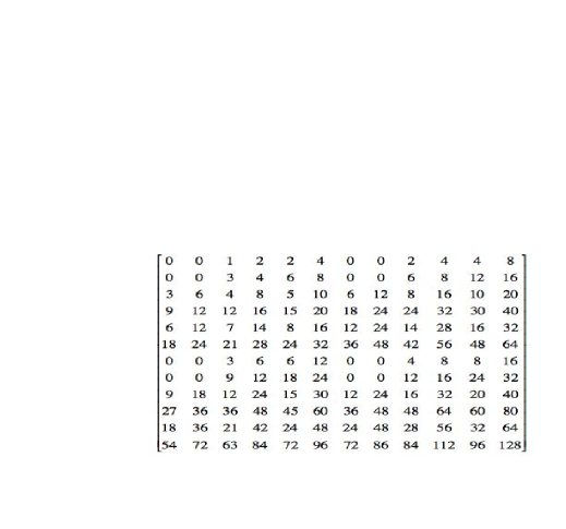
Figure 9:

Recall that the result matrix is filled in by 6, 2 x 2 blocks, over the rows and columns using the encoding discussed above. Notice how complicated the indirect addressing becomes using this approach to implementation of the Kronecker product. Notice also that if we wanted to distribute the computation of a block of rows to 4 processors, we’d need multiple components of the left argument.

Let us now look at doing the same operations, i.e. multiple outer products, using the MoA $\psi$ calculus approach, $C=A\,op_{\times}B$, as seen in Figure  10,

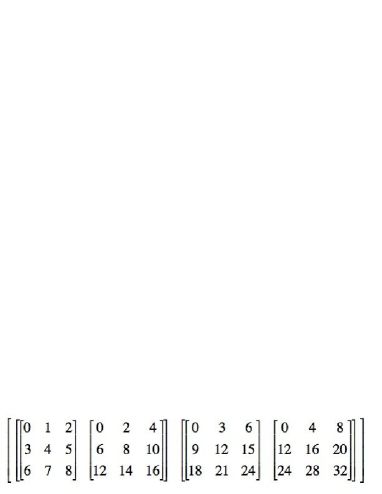
Figure 10:

is a 4-d array with shape 2 x 2 x 3 x 3. It is easy to see that indexing this array with partial indices yields 3 x 3 sub-arrays. That is, the indices, $<\!0\,0\!>$, $<\!0\,1\!>$, $<\!1\,0\!>$ and $<\!1\,1\!>$ are used to index C and each sub-array would be sent to available processors 0-3, to create a start, stop, stride, mapping suitable for all architectures to date.

Now let’s perform $C\,op_{\times}A$. This would yield a 6-d array with shape 2 x 2 x 3 x 3 x 2 x 2. We can easily pull apart the arguments in the operations. Let’s now think of this array as a 4 x 3 x 3 x 2 x 2. We then use the 4 to index the processors. We know the blocks have 36 components.

The following expressions illustrate how easy it is to compose, map, and scale to a multi-processor architecture. We first get the shape.

$$\rho((A\;op\;B)\;op\;A) = (\rho(A\;op\;B)+\!\!\!+(\rho A))$$

$$= (\rho A)+\!\!\!+(\rho B)+\!\!\!+(\rho A)$$

$$= <2\;2\;3\;3\;2\;2>$$

The indices are composed as follows: Given $0\leq^{*}\;\;<\!i\;j\!>\;\;<^{*}\;\;<\!2\;2\!>$; $0\leq^{*}\;\;<\!k\;l\!>\;\;<^{*}\;\;<\!3\;3\!>$; and $0\leq^{*}\;\;<\!m\;n\!>\;\;<^{*}\;\;<\!2\;2\!>$ and for all $0\leq^{*}\;\;<\!i\;j\;k\;l\;m\;n\!>\;\;<^{*}\;\;<\!2\;2\;3\;3\;2\;2\!>$;

$$<i\;j\;k\;l\;m\;n>\psi\;((A\;op_{\times}\;B)\;op_{\times}\;A) = (<i\;j\;k\;l>\psi\;(A\;op_{\times}\;B))\times(<m\;n>\psi A)$$

$$= (<i\;j>\psi A)\;\times(<k\;l>\psi B)\;\times(<m\;n>\psi A)$$

From here we can easily map chunks to the four processors using starts, stops, and strides.

Let’s take the above, referred to as the Denotational Normal Form (DNF) expressed in terms of Cartesian coordinates and transform it into its equivalent Operational Normal Form, (ONF), expressed in terms of start, stop, stride and count. The DNF is independent of layout. The ONF requires one. Let’s assume row-major. We’ll see how natural that is for the Kronecker product at all levels of implementation.

Let’s break up the above multiple Kronecker product over 4 processors. We’ll need to restructure the array’s shape $<2\;2\;3\;3\;2\;2>$, to $<4\;3\;3\;2\;2>$. This allows us to index the first dimension of this abstraction over the processors. We’ll also index the first component of the leftmost argument by this value. Notice that the entire right argument is used/accessed in all of the processors. Thus, we think of the entire result of both products residing in an array with $\;\pi<4\;3\;3\;2\;2>\;=144$ components (the $\pi$ operator gives the product of the elements of the vector) laid out contiguously in memory using a row-major ordering.

Thus the equation above becomes for $0\leq p<4$

$$<i\;j\;k\;l\;m\;n>\psi\;((A\;op_{\times}\;B)\;op_{\times}\;A) = <p\;k\;l\;m\;n>\psi\;((\vec{a}\;op_{\times}\;B)\;op_{\times}\;A$$

$$= ((<p>\psi\vec{a})\;\times(<k\;l>\psi B))\;\times(<m\;n>\psi A)$$

The expression below describes what each processor, $p$, will do. $\vec{a}$ above denotes the restructuring of $A$. avec and bvec are used to describe generic implementations. $\forall\;p,q,r\;\;s.t.\;0\leq p<4\;;\;0\leq q<9;\;\;0\leq r<4$

  ( avec[p] x bvec[q ]) x avec[r]
   

We are able to collapse the 2-d indexing for A and B since their access is contiguous. This type of thinking and reasoning has been used for over 20 years[6, 7, 8].

5 Conclusion

The purpose of this paper was to illustrate how the Kronecker product/outer product is implemented, i.e. the algorithm used to represent the Kronecker/Tensor product, can hinder or exploit reasoning of resource management, performance, scalability, and portability of the algorithm. The classical way works but is not easy to represent, compose, and partition over processor/memory hierarchies.

MoA and Psi Calculus provide a way to reason about array based computing. By using shapes and the $\psi$ function to define a small algebra, higher order operations can be defined, composed, optimized, and mapped to a simple machine abstraction: start, stop, stride, count.

Moving the theory to implementations that automatically generate correct optimal code is the next step. Over 20 years have been spent building prototypes to show proof of concept. Serious implementations must be initiated, studied, and advanced.

Appendix A Motivation for diadics, Kronecker and outer products

This section provides some simple examples of how dyadics and Kronecker products arise naturally in applied problems.

A.1 Example from engineering

In the field of electricity and magnetism the following operator arises in the wave equation for the electric field:

$$\nabla\times\nabla\times{\vec{E}}=-\nabla^{2}{\vec{E}}+\nabla(\nabla\cdot{\vec{E}}).$$ (25)

For a known source current density $\vec{J}({\vec{r}},t)$ (with a known Fourier expansion) it is natural to expand the electric field in a Fourier expansion. Thus we are let to consider the action of the operator of Eq. 25 on a single Fourier component:

$${\vec{E}}_{({\vec{q}},\omega)}({\vec{r}},t)={\vec{E}}({\vec{q}},\omega)\exp(i({\vec{q}}\cdot{\vec{r}}-\omega t))$$ (26)

Action on Eq. 26 with the operator of Eq. 25 gives:

$$q^{2}{\vec{E}}-{\vec{q}}({\vec{q}}\cdot{\vec{E}}).$$ (27)

This is simplified by introducing the dyadic (or Kronecker product): ${\vec{q}}\otimes{\vec{q}}$, by writing:

$$q^{2}{\vec{E}}-{\vec{q}}({\vec{q}}\cdot{\vec{E}})\equiv(q^{2}{\hat{I}}-{\vec{q}}\otimes{\vec{q}})\cdot{\vec{E}},$$ (28)

where $\hat{I}$ is the unit tensor (matrix) and the dyadic ${\vec{q}}\otimes{\vec{q}}$, is defined by its action on any other vector $\vec{u}$ as follows:

$$({\vec{q}}\otimes{\vec{q}})\cdot{\vec{u}}\equiv{\vec{q}}({\vec{q}}\cdot{\vec{u}}).$$ (29)

A convenient interpretation of the dyadic ${\vec{q}}\otimes{\vec{q}}$, arises if we work with the unit vector ${\hat{q}}\equiv{\vec{q}}/q$, where $q$ is the magnitude of the vector $\vec{q}$. In terms of the unit vector $\hat{q}$, Eq. 28, becomes:

$$q^{2}{\vec{E}}-{\vec{q}}({\vec{q}}\cdot{\vec{E}})\equiv q^{2}({\hat{I}}-{\hat{q}}\otimes{\hat{q}})\cdot{\vec{E}},$$ (30)

and we recognize the operator in parenthesis on the right hand side of Eq. 30 as a projection operator.

Indeed, the vector $({\hat{q}}\otimes{\hat{q}})\cdot{\vec{E}}$ represents the component of $\vec{E}$ along the direction of $\hat{q}$ and the vector $({\hat{I}}-{\hat{q}}\otimes{\hat{q}})\cdot{\vec{E}}$ represents the component of $\vec{E}$ perpendicular to $\hat{q}$. Explicitly we see

$$({\hat{I}}-{\hat{q}}\otimes{\hat{q}})\cdot({\hat{q}}\otimes{\hat{q}})=0.$$ (31)

This follows from

$$({\hat{q}}\otimes{\hat{q}})\cdot({\hat{q}}\otimes{\hat{q}})={\hat{q}}\otimes{\hat{q}},$$ (32)

which is a natural consequence of the above definitions.

Another contribution to the equation for electromagnetic waves in an anisotropic medium is the displacement field $\vec{D}$ that is related to the electric field $\vec{E}$ by the equation:

$${\vec{D}}={\bar{\epsilon}}\cdot{\vec{E}},$$ (33)

where $\bar{\epsilon}$ is the dielectric tensor with diagonal components $\bar{\epsilon}_{||}$ and off-diagonal components $\bar{\epsilon}_{\perp}$. The components $\bar{\epsilon}_{||}$ and $\bar{\epsilon}_{\perp}$ arise from the fact that the response of the medium is different for electric field components parallel to, and perpendicular to the direction of wave propagation $\hat{q}$, respectively.

Using the dyadic notation, the dielectric tensor $\bar{\epsilon}$ is conveniently written as

$${\bar{\epsilon}}={\bar{\epsilon}_{||}}({\hat{q}}\otimes{\hat{q}})+{\bar{\epsilon}_{\perp}}({\hat{I}}-{\hat{q}}\otimes{\hat{q}}).$$ (34)

The complete wave equation, in Fourier space, reads:

$${\bar{A}}({\vec{q}},\omega)\cdot{\vec{E}}({\vec{q}},\omega)={\vec{b}}({\vec{q}},\omega)$$ (35)

where the operator ${\bar{A}}({\vec{q}},\omega)$ is the sum of the longitudinal component:

$${\bar{A}}_{||}({\vec{q}},\omega)={\frac{\omega^{2}{\bar{\epsilon}_{||}({\vec{q}},\omega)}}{c^{2}}}({\hat{q}}\otimes{\hat{q}}),$$ (36)

and the transverse component:

$${\bar{A}}_{\perp}({\vec{q}},\omega)=\Biggl{(}{\frac{\omega^{2}{\bar{\epsilon}_{\perp}({\vec{q}},\omega)}}{c^{2}}-q^{2}}\Biggr{)}({\hat{I}}-{\hat{q}}\otimes{\hat{q}}).$$ (37)

The right hand side of the wave equation (Eq. 35) is defined in terms of the known current density ${\vec{J}}({\vec{q}},\omega)$ by:

$${\vec{b}}({\vec{q}},\omega)\equiv{\frac{4\pi i\omega}{c^{2}}}{\vec{J}}({\vec{q}},\omega)$$ (38)

The wave equation (Eq. 35) is solved through the use of the dyadic Green’s function ${\bar{G}}({\vec{q}},\omega)$

$${\vec{E}}({\vec{q}},\omega)={\vec{G}}({\vec{q}},\omega)\cdot{\vec{b}}({\vec{q}},\omega),$$ (39)

where ${\vec{G}}({\vec{q}},\omega)$ is the inverse of ${\vec{A}}({\vec{q}},\omega)$ and thus satisfies:

$${\vec{G}}({\vec{q}},\omega)\cdot{\vec{A}}({\vec{q}},\omega)={\hat{I}}.$$ (40)

The longitudinal and transverse components of the dyadic Green’s function are given explicitly by:

$${\bar{G}}_{||}({\vec{q}},\omega)={\frac{({\hat{q}}\otimes{\hat{q}})}{\Bigl{(}{\frac{\omega^{2}{\bar{\epsilon}_{||}({\vec{q}},\omega)}}{c^{2}}}\Bigr{)}}},$$ (41)

and,

$${\bar{G}}_{\perp}({\vec{q}},\omega)={\frac{({\hat{I}}-{\hat{q}}\otimes{\hat{q}})}{\Biggl{(}{\frac{\omega^{2}{\bar{\epsilon}_{\perp}({\vec{q}},\omega)}}{c^{2}}-q^{2}}\Biggr{)}}}.$$ (42)

Thus a complete solution of the original problem is obtained by Fourier transforming Eq. 39.

A.2 Example from linear algebra: matrix decompositions

Kronecker products (dyadics) can also be conveniently used to express a matrix expansion. Consider a Hermitian matrix $H$ and its normalized eigenvectors ${\vec{u}}_{j}$ (i.e. ${\vec{u}_{i}}{\vec{u}_{j}}=\delta_{ij}$) and eigenvalues $\lambda_{j}$ satisfying $Hu_{j}=\lambda_{j}u_{j}$.

A well-known result of linear algebra is that the matrix $H$ can be expressed in terms of the following expansion involving Kronecker products:

$$H=\lambda_{1}{\vec{u}_{1}}\otimes{\vec{u}_{1}},+\lambda_{2}{\vec{u}_{2}}\otimes{\vec{u}_{2}}+\cdots.$$ (43)

This expansion follows from the fact that the eigenvectors form a complete basis and, as such, any arbitrary vector can be expanded as a sum of the eigenvectors as:

$${\vec{v}}=c_{1}{\vec{u}_{1}}+c_{2}{\vec{u}_{2}}+\cdots$$ (44)

We see again, the natural interpretation of the Kronecker products as projection operators. Each term in the expansion of Eq. 43 gives a non-zero result only when acting on the corresponding eigenvector of Eq. 44. The result, $\lambda_{j}c_{j}{\vec{u}_{j}}$, is identical to the action of $H$ acting on the corresponding component $c_{1}{\vec{u}_{1}}$ in the vector expansion of Eq. 44. In other words, we find

$$({\vec{u}_{i}}\otimes{\vec{u}_{i}})\cdot{\vec{u}_{j}}=\delta_{ij}{\vec{u}_{i}}.$$ (45)

Thus, this section is consistent with the previous section in terms of the interpretation of Kronecker products as projection operators.

A.3 Higher dimensional generalizations

We now consider an example from the theory of orthogonal functions (i.e. Hilbert space). For this discussion, it is convenient to use Dirac notation. We expand a given function $|\psi\!>$ in a complete set of basis functions $|\ell,m\!>$ as:

$$|\psi\!>=\sum_{\ell,m}C_{\ell,m}|\ell,m\!>.$$ (46)

By orthogonality we see that the coefficients can be written in terms of an inner product:

$$C_{\ell,m}=<\!\ell,m|\psi\!>,$$ (47)

which is interpreted as a projection onto the basis vector (function) $|\ell,m\!>$. We now wish to expand in another complete basis set $|\ell^{\prime},m^{\prime}\!>$, perhaps obtained from the starting set by rotating the coordinate system

$$|\psi\!>=\sum_{\ell^{\prime},m^{\prime}}B_{\ell^{\prime},m^{\prime}}|\ell^{\prime},m^{\prime}\!>.$$ (48)

The coefficients of this expansion are likewise expressed as:

$$B_{\ell^{\prime},m^{\prime}}=<\!\ell^{\prime},m^{\prime}|\psi\!>,$$ (49)

and we can relate the coefficients of this later expansion to the coefficients the former expansion by taking the inner product of Eq. 48 with the basis function $|\ell,m\!>$, to yield:

$$<\!\ell,m|\psi\!>=\sum_{\ell^{\prime},m^{\prime}}<\ell,m|\ell^{\prime},m^{\prime}\!><\ell^{\prime},m^{\prime}|\psi>,$$ (50)

which can more simply be written:

$$C_{\ell,m}=\sum_{\ell^{\prime},m^{\prime}}<\ell,m|\ell^{\prime},m^{\prime}\!>B_{\ell^{\prime},m^{\prime}}$$ (51)

From equations 50 and 51 we see the natural definition of the unit operator:

$${\hat{I}}=\sum_{\ell^{\prime},m^{\prime}}|\ell^{\prime},m^{\prime}\!><\ell^{\prime},m^{\prime}|$$ (52)

Note the close analogy between this expansion and the expansion of the Hermitian matrix in terms of its eigenvectors in Eq. 43. We see therefore, that a higher-dimensional analog of Eq. 43 would be the operator expansion of

$${\hat{L}}=\sum_{\ell^{\prime},m^{\prime}}\lambda_{\ell,m}|\ell^{\prime},m^{\prime}\!><\ell^{\prime},m^{\prime}|,$$ (53)

where $\lambda_{\ell,m}$ and $|\ell,m\!>$ are the eigenvalues and eigenfunctions of the operator $\hat{L}$, respectively (i.e. ${\hat{L}}|\ell,m\!>=\lambda_{\ell,m}|\ell,m\!>$).

If we express operators such as Eq. 53 in matrix form, we are naturally led to a higher dimensional generalization of the dyadic ${\vec{u}}\otimes{\vec{u}}$, namely, the matrix product: ${\bar{A}}\otimes{\bar{A}}$, where $\bar{A}$ is a matrix or higher dimensional tensor. Compositions of such products, such as ${\bar{A}}\otimes{\bar{B}}\otimes{\bar{C}}$ are also similarly defined.

A.4 Matrix form

The matrix representation of the Kronecker Product is

$$({\bar{A}}\otimes{\bar{B}})_{I,J}=A_{i,j}B_{\ell,m}$$ (54)

where $I\equiv<i,\ell>$ and $J=<j,m>$ are composite indices that cycle through the integers as $<i,\ell>$ and $<j,m>$ cycle through their allowed values in row major order (i.e. $\ell$ cycles faster than $i$ and $m$ cycles faster than $j$), and the eigenvector $U_{J}$ is constructed as a large column vector with as many copies of the eigenvector $\vec{u}_{i}$ of $B$ as there are columns of $A$.

References

- [1] M. Davio. Kronecker products and shuffle algebra. IEEE Trans. Comput., c-30:116, 1981.
- [2] A. Graham. Kronecker Products and Matrix Calculus with Applications. Ellis Horwood, Chichester, England, 1981.
- [3] H.V. Henderson, F. Pukelsheim, and S.R. Searle. On the history of the kronecker product. Linear Multilinear Algebra, 14:113, 1983.
- [4] H.V. Henderson and S.R. Searle. The vec-permutation matrix, the vec operator and kronecker products: a review. Linear Multilinear Algebra, 9:271, 1981.
- [5] R. A. Horn and C. A. Johnson. Topics in Matrix Analysis. Cambridge University Press, New York, 1991.
- [6] L. M. R. Mullin. A Mathematics of Arrays. PhD thesis, Syracuse University, December 1988.
- [7] L. R. Mullin. A uniform way of reasoning about array–based computation in radar: Algebraically connecting the hardware/software boundary. Digital Signal Processing, 15:466–520, 2005.
- [8] L. R. Mullin and J. E. Raynolds. Conformal Computing: Algebraically connecting the hardware/software boundary using a uniform approach to high-performance computation for software and hardware applications. arXiv:0803.2386, 2008.
- [9] L.M. R. Mullin. Psi, the indexing function: A basis for FFP with arrays. In Arrays, Functional Languages, and Parallel Systems. Kluwer Academic Publishers, 1991.
- [10] P. A. Regalia and S. Mitra. Kronecker products, unitary matrices, and signal processing applications. SIAM Rev., 31:586, 1989.
- [11] R. A. Snay. Applicability of array algebra,. Rev. Geophys. Space Phys., 16:459, 1978.
- [12] W-H. Steeb. Matrix Calculus and Kronecker Product with Applications and C++ Programs. World Scientific Publishing, Singapore, 1997.
- [13] C. F. Van-Loan. The ubiquitous kronecker product. J. Comp. Appl. Math, 85:123, 2000.