A new cosmic shear function: Optimised E-/B-mode decomposition on a finite interval

Abstract

The decomposition of the cosmic shear field into E- and B-mode is an important diagnostic in weak gravitational lensing. However, commonly used techniques to perform this separation suffer from mode-mixing on very small or very large scales. We introduce a new E-/B-mode decomposition of the cosmic shear two-point correlation on a finite interval. This new statistic is optimised for cosmological applications, by maximising the signal-to-noise ratio (S/N) and a figure of merit (FoM) based on the Fisher matrix of the cosmological parameters $\Omega_{\rm m}$ and $\sigma_{8}$.

We improve both S/N and FoM results substantially with respect to the recently introduced ring statistic, which also provides E-/B-mode separation on a finite angular range. The S/N (FoM) is larger by a factor of three (two) on angular scales between 1 and 220 arc minutes. In addition, it yields better results than for the aperture-mass dispersion $\langle M_{\rm ap}^{2}\rangle$, with improvements of 20% (10%) for S/N (FoM). Our results depend on the survey parameters, most importantly on the covariance of the two-point shear correlation function. Although we assume parameters according to the CFHTLS-Wide survey, our method and optimisation scheme can be applied easily to any given survey settings and observing parameters. Arbitrary quantities, with respect to which the E-/B-mode filter is optimised, can be defined, therefore generalising the aim and context of the new shear statistic.

1 Introduction

Cosmic shear, the weak gravitational lensing effect induced on images of distant galaxies by the large-scale structure in the Universe, has become a standard tool for observational cosmology (see Schneider 2006; Hoekstra & Jain 2008; Munshi et al. 2008, for recent reviews). Large surveys have used cosmic shear to obtain measurements of the matter density $\Omega_{\rm m}$ and the density fluctuation amplitude $\sigma_{8}$. Recent constraints were obtained from ground-based surveys such as CFHTLS (Benjamin et al. 2007; Fu et al. 2008) and GaBoDS (Hetterscheidt et al. 2007). Space-based surveys like COSMOS (Leauthaud et al. 2007; Massey et al. 2007) and parallel ACS data (Schrabback et al. 2007) advanced cosmic shear observations to very small angular scales. Cosmic shear has contributed to constraining dark energy (Jarvis et al. 2006; Kilbinger et al. 2009). It is considered to be one of the most promising method to shed light onto the origin of the recent accelerated expansion of the Universe (Albrecht et al. 2006; Peacock et al. 2006), and is a major science driver for many future surveys like KIDS, Pan-STARRS, DES, LSST, JDEM or Euclid.

One of the (few) diagnostics for cosmic shear analyses is the decomposition of the shear field into its E- and B-mode. Most commonly, the shear power spectrum or, equivalently, the shear correlation function, is split into the gradient (E) and curl (B) component (Crittenden et al. 2002; Schneider et al. 2002). Gravitational lensing produces, to first order, a curl-free shear field and therefore, the presence of a B-mode is an indication of residual systematics in the PSF correction and shape measurement analysis. To obtain competitive constraints on cosmological parameters, in particular for dark-energy or beyond-standard physics, galaxy shapes have to be determined to sub-percentage precision. This requires excellent correction of PSF effects arising from the atmosphere, telescope and camera imperfections.

Apart from observational effects and measurement systematics, the cosmic shear signal can be severely contaminated by intrinsic correlations of galaxy orientation with other galaxies or their surrounding dark matter structures (Heavens et al. 2000). This occurs for galaxies at the same redshift e.g. which reside in the same dark halo (intrinsic alignment). It also affects galaxies at very different redshifts, where a background galaxy is lensed by matter surrounding a foreground galaxy, therefore inducing a shape-shear-correlation between the two galaxies. An E-mode as well as a B-mode arises from intrinsic alignment (Crittenden et al. 2002; Mackey et al. 2002).

Standard methods to separate the E- and B-mode power spectra (or correlation functions) involve integrals up to arbitrary small or large angular scales (Schneider et al. 1998; Crittenden et al. 2002; Schneider et al. 2002). However, shear correlations can be observed only on a finite interval. Since the shear field is probed at galaxy positions, the smallest usable scale is given by the confusion limit for close galaxy pairs, which is typically several arc minutes for ground-based surveys. The largest observed distance is for current surveys several degrees. These limits make the E-/B-mode separation imperfect, and a mixing of modes is induced at the 1-10% level (Kilbinger et al. 2006). To circumvent this shortcoming, a new second-order function, the so-called “ring statistic”, was introduced which permits a clear E-/B-mode separation on a finite interval (Schneider & Kilbinger 2007, hereafter SK07). In addition, the authors developed conditions for general filter functions necessary for an E-/B-mode decomposition for a finite angular range.

In this work, we present a method to find filter functions which fulfill the SK07 conditions. We devise a scheme which provides an optimised E-/B-mode decomposition on a finite interval. The optimisation is performed with regard to cosmological applications of cosmic shear; the signal-to-noise ratio and a Fisher matrix figure or merit are the quantities to be maximised. This paper is organised as follows: In Sect. 2 we briefly review the results from SK07 before we present our optimisation method. Results for the signal-to-noise ratio and the figure of merit are shown in Sect. 3. We conclude the paper with a summary (Sect. 4) and an outlook (Sect. 5).

2 Method

2.1 E-and B-mode Decomposition of the shear correlation function on a finite interval

We define the general second-order cosmic shear functions ${\cal R}_{\rm E}$ and ${\cal R}_{\rm B}$,

$${\cal R}_{\rm E} =\frac{1}{2}\int_{0}^{\infty}{\mathrm{d}}\vartheta\,\vartheta\left[T_{+}(\vartheta)\,\xi_{+}(\vartheta)+T_{-}(\vartheta)\,\xi_{-}(\vartheta)\right];$$

$${\cal R}_{\rm B} =\frac{1}{2}\int_{0}^{\infty}{\mathrm{d}}\vartheta\,\vartheta\left[T_{+}(\vartheta)\,\xi_{+}(\vartheta)-T_{-}(\vartheta)\,\xi_{-}(\vartheta)\right],$$ (1)

as integrals over the shear two-point correlation functions $\xi_{+}$ and $\xi_{-}$ (e.g. Kaiser 1992) with arbitrary filter functions $T_{+}$ and $T_{-}$. These expressions correspond to Eq. (39) from SK07, with an additional factor $1/2$ in our definition. In terms of the E- and B-mode power spectrum, $P_{\rm E}$ and $P_{\rm B}$, respectively, the shear two-point correlation function are given as the following Hankel transforms (Schneider et al. 2002)

$$\xi_{+}(\vartheta) =\int_{0}^{\infty}{{\mathrm{d}}\ell\;\ell\over 2\pi}\,{\rm J_{0}}(\ell\vartheta)[{P_{\rm E}(\ell)+P_{\rm B}(\ell)}];$$

$$\xi_{-}(\vartheta) =\int_{0}^{\infty}{{\mathrm{d}}\ell\;\ell\over 2\pi}\,{\rm J_{4}}(\ell\vartheta)[{P_{\rm E}(\ell)-P_{\rm B}(\ell)}].$$ (2)

with ${\mathrm{J}}_{\nu}$ being the $\nu^{\rm th}$-order Bessel function of the first kind. Inserting Eq. (2) into Eq. (1) yields

$${\cal R}_{\rm E}=\frac{1}{2}\int_{0}^{\infty}\frac{{\mathrm{d}}\ell\,\ell}{{2\pi}}\Bigg{[} P_{\rm E}(\ell)\Big{(}{\cal W}_{\rm E}(\ell)+{\cal W}_{\rm B}(\ell)\Big{)}$$

$$+ P_{\rm B}(\ell)\Big{(}{\cal W}_{\rm E}(\ell)-{\cal W}_{\rm B}(\ell)\Big{)}\Bigg{]},$$ (3)

and an analogous expression for ${\cal R}_{\rm B}$. The Hankel transforms of $T_{+}$ and $T_{-}$ are defined as

$${\cal W}_{\rm E,B}(\ell)=\int_{0}^{\infty}{\mathrm{d}}\vartheta\,\vartheta\,T_{+,-}(\vartheta)\,{\mathrm{J}}_{0,4}(\vartheta\ell).$$ (4)

To provide an E- and B-mode decomposition, in the sense that ${\cal R}_{\rm E}$ only depends on the E-mode of the shear field and ${\cal R}_{\rm B}$ only on its B-mode, the two Hankel transform have to be identical, ${\cal W}_{\rm E}={\cal W}_{\rm B}$. After some algebra, one finds that the following equivalent relations between the filter functions $T_{+}$ and $T_{-}$ must hold (Schneider et al. 2002)

$$T_{+}(\vartheta) =T_{-}(\vartheta)+4\int_{\vartheta}^{\infty}\frac{{\mathrm{d}}\theta\,\theta}{\theta^{2}}\,T_{-}(\theta)\left[1-3\left(\frac{\vartheta}{\theta}\right)^{2}\right];$$ (5)

$$T_{-}(\vartheta) =T_{+}(\vartheta)+4\int_{0}^{\vartheta}\frac{{\mathrm{d}}\theta\,\theta}{\vartheta^{2}}\,T_{+}(\theta)\left[1-3\left(\frac{\theta}{\vartheta}\right)^{2}\right].$$ (6)

Therefore, for an arbitrary function $T_{+}$, a corresponding filter $T_{-}$ can be derived from $T_{+}$ to provide an E- and B-mode decomposition, and vice versa. In the absence of a B-mode we have ${\cal R}_{\rm B}=0$, and ${\cal R}_{\rm E}$ can be obtained from $\xi_{+}$ or $\xi_{-}$ alone,

$${\cal R}_{\rm E}=\int_{0}^{\infty}{\mathrm{d}}\vartheta\,\vartheta\,T_{+}(\vartheta)\,\xi_{+}(\vartheta)=\int_{0}^{\infty}{\mathrm{d}}\vartheta\,\vartheta\,T_{-}(\vartheta)\,\xi_{-}(\vartheta).$$ (7)

We further require ${\cal R}_{\rm E}$ and ${\cal R}_{\rm B}$ to depend on the shear correlation given at angular scales $\vartheta$ in a finite interval, $0<\vartheta_{\rm min}\leq\vartheta\leq\vartheta_{\rm max}<\infty$. Thus, we demand $T_{-}$ to have finite support $[\vartheta_{\rm min};\vartheta_{\rm max}]$ and $T_{+}(\vartheta)$ to vanish for $\vartheta<\vartheta_{\rm min}$, Eq. (5) then implies the following integral constraints on the filter function $T_{-}$ (SK07):

$$\int_{\vartheta_{\rm min}}^{\vartheta_{\rm max}}\frac{{\mathrm{d}}\vartheta}{\vartheta}T_{-}(\vartheta)=\int_{\vartheta_{\rm min}}^{\vartheta_{\rm max}}\frac{{\mathrm{d}}\vartheta}{\vartheta^{3}}T_{-}(\vartheta)=0.$$ (8)

In addition, it follows that $T_{+}(\vartheta)=0$ for $\vartheta>\vartheta_{\rm max}$. Using the finite support of $T_{+}$ in (Eq. 6), we get integral constraints for $T_{+}$,

$$\int_{\vartheta_{\rm min}}^{\vartheta_{\rm max}}{\mathrm{d}}\vartheta\,\vartheta T_{+}(\vartheta)=\int_{\vartheta_{\rm min}}^{\vartheta_{\rm max}}{\mathrm{d}}\vartheta\,\vartheta^{3}T_{+}(\vartheta)=0.$$ (9)

Then, ${\cal R}_{\rm E}$ and ${\cal R}_{\rm B}$ are functions of the two angular scales $\vartheta_{\rm min}$ and $\vartheta_{\rm max}$. We will discuss the scale-dependence in more detail in Sect. 2.6.

SK07 constructed a set of functions, $Z_{+},Z_{-}$ in their notation, which satisfy Eqs. (8, 9). Those functions were motivated from a geometrical ansatz, by considering two concentric, non-overlapping rings. If the shear correlation is calculated from galaxy pairs of which one galaxy lies in the inner ring and the other galaxy in the outer ring, the E-/B-mode decomposition on a finite interval is guaranteed by construction. The form of the function $Z_{+}$ originated in a specific choice of the weight profile over the two rings. The relation between $T_{\pm}$ and $Z_{\pm}$ is

$$T_{\pm}(\vartheta)=\vartheta^{-2}\,Z_{\pm}(\vartheta/\vartheta_{\rm max}).$$ (10)

Note that in SK07 the analogous integrals to Eq. (1) using $Z_{\pm}$ are carried out over the integration variable $\vartheta/\vartheta_{\rm max}$ and extend from $\vartheta_{\rm min}/\vartheta_{\rm max}$ to 1. The shear second-order functions corresponding to Eq. (1) are denoted as $\langle{\cal RR}\rangle_{\rm E}$ and $\langle{\cal RR}\rangle_{\rm B}$, respectively.

There are infinitely many functions which fulfill the above integral constraints. Their choice can of course be detached from the geometrical considerations of the “ring statistic”. In this paper we define a general filter function which we will optimise regarding some specific criterion. This criterion will be related to the cosmological information output from a cosmic shear survey. We will use two cases, the signal-to-noise ratio and the Fisher matrix of cosmological parameters. The results are presented in Sect. 3.

2.2 Parametrisation of the filter function

For the optimisation problem, we focus on $T_{+}$ since $T_{-}$ can be derived from $T_{+}$ (Eq. 6). First, we remap $T_{+}$ to the interval $[-1;+1]$ by defining

$$\tilde{T}_{+}(x)= \,T_{+}(Ax+B)=T_{+}(\vartheta)\quad\mbox{for}\quad x\in[-1;1];$$

$$A= \,(\vartheta_{\rm max}-\vartheta_{\rm min})/2;\;\;\;B=(\vartheta_{\rm max}+\vartheta_{\rm min})/2.$$ (11)

With that the two integral constraints (Eq. 9) become

$$\int_{-1}^{+1}{\mathrm{d}}x\,(x+R)\,\tilde{T}_{+}(x)=\int_{-1}^{+1}{\mathrm{d}}x\,(x+R)^{3}\,\tilde{T}_{+}(x)=0,$$ (12)

where we have defined the ratio $R$ as

$$R=\frac{B}{A}=\frac{1+\eta}{1-\eta};\;\;\;\;\eta=\frac{\vartheta_{\rm min}}{\vartheta_{\rm max}}.$$ (13)

Next, we decompose $\tilde{T}_{+}$ into a finite sum of orthogonal polynomials:

$$\tilde{T}_{+}(x)=\sum_{n=0}^{N-1}a_{n}\,C_{n}(x).$$ (14)

This representation allows us to find an optimal filter function by varying the coefficients $a_{n}$. Sect. 2.7. The polynomials $C_{n}$ can be chosen freely; we use Chebyshev polynomials of the second kind,

$${\rm U}_{n}(x)=\frac{\sin[(n+1)\arccos x]}{\sin(\arccos x)}.$$ (15)

The optimisation process is then performed by varying the coefficients $a_{n}$; this is described in detail in Sect. 2.7.

Apart from the integral constraints (Eq. 9), one could require $T_{+}$ to be zero at the interval boundaries,

$$\mbox{Continuity}:\quad T_{+}(\vartheta_{\rm max})=T_{+}(\vartheta_{\rm min})=0.$$ (16)

Additional constraints could be added, for example differentiability at the boundaries. We will discuss their effects on the results in Sect. 3.1.

2.3 Satisfying the constraints

In general, the function $T_{+}$, or equivalently $\tilde{T}_{+}$, is constrained by $K\geq 2$ equations in the form $F_{m}[\tilde{T}_{+}]=0,\;m=0\ldots K-1$. If the functionals $F_{m}$ are linear in $\tilde{T}_{+}$, applying Eq. (14) leads to

$$\sum_{n=0}^{N-1}f_{mn}\,a_{n}=0;\;\;\;\;f_{mn}:=F_{m}[C_{n}].$$ (17)

The matrix element $f_{mn}$ is the $m^{\rm th}$ constraint applied to the orthogonal polynomial of order $n$. For example, taking the first constraint in Eq. (12) we get

$$f_{0n}=\int_{-1}^{+1}{\mathrm{d}}x\,(x+R)\,C_{n}(x),$$ (18)

which can be integrated analytically. The other matrix elements $f_{mn}$ are obtained analogously.

$K$ constraints fix $K$ coefficients of the decomposition (Eq. 14), the remaining $N-K$ coefficients can be chosen arbitrarily. We use the highest $N-K$ coefficients as free parameters ($n=K\ldots N-1$) and fix the first $K$ coefficients ($n=0\ldots K-1$) as follows. Define

$$s_{m}=-\sum_{n=K}^{N-1}f_{mn}\,a_{n};\;\;\;\;m=0\ldots K-1,$$ (19)

Eq. (17) can then be written as

$$\sum_{n=0}^{K-1}f_{mn}\,a_{n}=s_{m};\;\;\;\;m=0\ldots K-1.$$ (20)

This $(K\times K)$-matrix equation is solved for the first $K$ coefficients $a_{n}\,(n=0\ldots K-1)$ by inverting the square (sub-)matrix $(f_{mn})_{m,n<K}$ on the left-hand side of the above equation. If the constraints are chosen such that they are linearly independent (which is this case), this matrix equation has a unique, non-trivial solution.

In addition to the $K$ constraints, we impose an integral normalisation of the filter function given by the $L^{2}$-norm

$$||\tilde{T}_{+}||^{2}_{2}=\int_{-1}^{1}{\mathrm{d}}x\,w(x)\tilde{T}_{+}^{2}(x)=1,$$ (21)

where $w$ is the corresponding weight of the polynomial family, $w(x)=(1-x^{2})^{1/2}$ in the case of second-kind Chebyshev polynomials. This normalisation does not affect the constraints which are independent of a multiplication of all $a_{n}$ with a common factor. Note also that the quantities which we will optimise in Sect. 3 do not depend on the normalisation.

2.4 Calculation of $T_{-}$ from $T_{+}$

To obtain the function $\tilde{T}_{-}:=T_{-}(Ax+B)$ we transform Eq. (6) to

$$\tilde{T}_{-}(x)= \,\tilde{T}_{+}(x)+4\int_{-1}^{x}{\mathrm{d}}x^{\prime}\,\tilde{T}_{+}(x^{\prime})\frac{x^{\prime}+R}{(x+R)^{2}}\,\left[1-3\left(\frac{x^{\prime}+R}{x+R}\right)^{2}\right];$$

$$x=-1\ldots 1,$$ (22)

which can be written as

$$\tilde{T}_{-}(x)= \sum_{n=0}^{N-1}a_{n}\left[C_{n}(x)+\alpha_{n}(x)\right];$$ (23)

$$\alpha_{n}(x)= \,4\int_{-1}^{x}{\mathrm{d}}x^{\prime}\,C_{n}(x^{\prime})\frac{x^{\prime}+R}{(x+R)^{2}}\,\left[1-3\left(\frac{x^{\prime}+R}{x+R}\right)^{2}\right],$$ (24)

inserting the decomposition (Eq. 14). We define

$$F_{n}^{(\nu)}(x)=\int_{-1}^{x}{\mathrm{d}}x^{\prime}\,(x^{\prime})^{\nu}C_{n}(x^{\prime});\;\;\;\;\nu=0,1,2,3,$$ (25)

and write Eq. (24) as

$$\alpha_{n}(x)= \frac{4}{3}r\left[R(r-R)F_{n}^{(0)}+(1-2rR-rR^{2})F_{n}^{(1)}\right.$$

$$\left.-rR(R+2)F_{n}^{(2)}-rF_{n}^{(3)}\right];$$

$$r= \frac{3}{(x+R)^{2}},$$ (26)

where we dropped the argument $x$ from $F_{n}^{(\nu)}$ and $r$. The integral (Eq. 25) for $\nu=0$ and $C_{n}={\rm U}_{n}$ is

$$F_{n}^{(0)}(x)=\left\{\begin{array}[]{ll}\frac{\displaystyle(-1)^{n}+x\,{\rm T}_{n}(x)-(1-x^{2}){\rm U}_{n-1}(x)}{\displaystyle n+1}&(n\neq-1)\\[10.00002pt] 0&(n=-1)\end{array}\right.,$$ (29)

where ${\rm T}_{n}$ is $n^{\rm th}$-order Chebyshev polynomial of the first kind,

$${\rm T}_{n}(x)=\cos(n\arccos x).$$ (30)

By using the recurrence relation of the Chebyshev polynomials, we obtain the other functions,

$$F_{n}^{(1)}= \frac{1}{2}\left[F_{n+1}^{(0)}+F_{n-1}^{(0)}\right];$$

$$F_{n}^{(2)}= \frac{1}{4}\left[F_{n+2}^{(0)}+2F_{n}^{(0)}+F_{n-2}^{(0)}\right];$$ (31)

$$F_{n}^{(3)}= \frac{1}{8}\left[F_{n+3}^{(0)}+3F_{n+1}^{(0)}+3F_{n-1}^{(0)}+F_{n-3}^{(0)}\right].$$

Note that Eq. (29) is valid for integer $n$, since the expressions for the orthogonal polynomials are well-defined for negative $n$.

With that, it can be readily checked whether the coefficients $a_{n}$ obtained with the method described in Sect. 2.3 and the resulting filter functions $\tilde{T}_{\pm}$ indeed provide an E-/B-mode decomposition, by verifying that the B-mode ${\cal R}_{\rm B}$ (Eq. 1) is zero. In Sect. 3.6 we discuss numerical issues when calculating the B-mode.

2.5 Relation to the lensing power spectrum

Eq. (3) shows the relation of ${\cal R}_{\rm E}$ to the power spectrum. Assuming a pure E-mode, this equation reads

$${\cal R}_{\rm E}=\frac{1}{2\pi}\int_{0}^{\infty}{\mathrm{d}}\ell\,\ell P_{\rm E}(\ell)\,{\cal W}_{\rm E}(\ell),$$ (32)

where the Fourier-space filter function $\cal W_{\rm E}$ can be written as

$${\cal W}_{\rm E}(\ell,\vartheta_{\rm min},\vartheta_{\rm max}) =\sum_{n=0}^{N-1}a_{n}{\cal W}_{n}(\ell,\vartheta_{\rm min},\vartheta_{\rm max});$$ (33)

$${\cal W}_{n}(\ell,\vartheta_{\rm min},\vartheta_{\rm max}) =\int_{\vartheta_{\rm min}}^{\vartheta_{\rm max}}{\mathrm{d}}\vartheta\,\vartheta\,C_{n}[(\vartheta-B)/A]\,\rm J_{0}(\vartheta\ell),$$ (34)

with $A$ and $B$ given in Eq. (11). Analogously, ${\cal R}_{\rm B}$ can be written in terms of the B-mode power spectrum $P_{\rm B}$

$${\cal R}_{\rm B}=\frac{1}{2\pi}\int_{0}^{\infty}{\mathrm{d}}\ell\,\ell P_{\rm B}(\ell)\,{\cal W}_{\rm B}(\ell,\vartheta_{\rm min},\vartheta_{\rm max}),$$ (35)

with ${\cal W}_{\rm E}={\cal W}_{\rm B}$, see Sect. 2.1.

Unfortunately there is no simple analytical expression of Eq. (34), which would be desirable to calculate Eq. (32) using a fast Hankel transform (FHT, Hamilton 2000). For the moment, the most efficient method to calculate ${\cal R}_{\rm E}$ from a model power spectrum is to obtain $\xi_{+}$ from $P_{\rm E}$ by FHT and to integrate it via Eq. (7) which is fast since in our case $T_{+}$ is a rather low-order polynomial, as we will see later.

2.6 Angular-scale-dependence

The two constraints (Eq. 9) depend on the ratio of angular scales $\eta=\vartheta_{\rm min}/\vartheta_{\rm max}$. A filter function $\tilde{T}_{+}$ with given coefficients $a_{n}$ satisfying those constraints does not in general fulfill the same constraints for a different $\eta$. This therefore causes the inconvenience of having a different filter function for each angular scale.

It should be noted that although formally ${\cal R}_{\rm E}$ is a function of two angular scales, the information about cosmology and large-scale structure is captured by a single parameter, let us call it $\lambda$. This is because the large-scale matter power spectrum, of which ${\cal R}_{\rm E}$ is a logarithmic convolution (Sect. 2.5), only depends on a single scalar. We therefore expect a large covariance between many pairs $(\vartheta_{\rm min},\vartheta_{\rm max})$. Although there are infinitely many mappings $(\vartheta_{\rm min},\vartheta_{\rm max})\rightarrow\lambda$, two ways to handle the scale-dependence seem to be suitable: (1) Leaving one scale constant, and varying the other scale, e.g. $\vartheta_{\rm min}=\mbox{const.},\lambda=\vartheta_{\rm max}$. (2) Leaving the ratio of both scales constant, $\lambda=\eta$. We will pursue both ways in this paper.

2.6.1 Fixed minimum scale, $\vartheta_{\rm min}={\rm const}$

The first mapping introduced above offers a rather efficient sampling of the shear field. $\vartheta_{\rm min}$ can be fixed to the smallest observable distance $\vartheta_{\rm min,0}$ for which shear correlation data are measured. This is given by the smallest separation for which galaxies do not blend, to allow for reliably measured shapes. It provides the largest range of angular scales accessible for a given $\vartheta_{\rm max}$: The upper limit $\vartheta_{\rm max}$ can be varied between $\vartheta_{\rm min}$ and the maximum observed scale given by the data.

2.6.2 Fixed ratio, $\eta=\vartheta_{\rm min}/\vartheta_{\rm max}={\rm const}$

The second mapping has the advantage that a single filter function can satisfy the constraints (Eq. 9) for all scales. This makes it more convenient to combine different scales, e.g. to obtain the Fisher matrix, and might result in a universal optimal filter function. The efficiency with respect to keeping $\vartheta_{\rm min}$ constant is however reduced: A large ratio $\eta$, for which $\vartheta_{\rm min}$ and $\vartheta_{\rm max}$ are close, samples only a small angular interval, resulting in a small signal-to-noise. A small $\eta$ on the other hand means that we can not go to very small scales with $\vartheta_{\rm max}$: Because of the minimum observable galaxy separation $\vartheta_{\rm min,0}$, the smallest $\vartheta_{\rm max}$ is $\mbox{min}(\vartheta_{\rm max})=\vartheta_{\rm min,0}/\eta$.

In both cases, we will use $\vartheta_{\rm max}$ as the argument of ${\cal R}_{\rm E}$ and denote it with the symbol $\Psi$, as in SK07.

In Appendix A, we introduce a simple generalisation of this scheme to obtain an optimised function $\tilde{T}_{+}$ which fulfills the integral constraints (Eq. 9) for all pairs $(\vartheta_{\rm min},\vartheta_{\rm max})$. However, the corresponding signal-to-noise ratio is significantly lower than with the method used here, which was presented in Sect. 2.3. We therefore do not consider this option further.

A remark about the analogy to the aperture-mass dispersion $\langle M_{\rm ap}^{2}\rangle$ is appropriate here. $\langle M_{\rm ap}^{2}\rangle$ is obtained from the correlation function in a similar way as ${\cal R}_{\rm E}$ in Eq. (1), with integration range between zero and twice the aperture radius. Its filter function depends on the two scales $\vartheta$ (the integration variable) and $\theta$ (the aperture radius). For different $\theta$ one could define a different filter function. For convenience however, widely-used filters are functions of the ratio $\vartheta/\theta$, and therefore one functional form provides an E-/B-mode separation for all radii simultaneously.

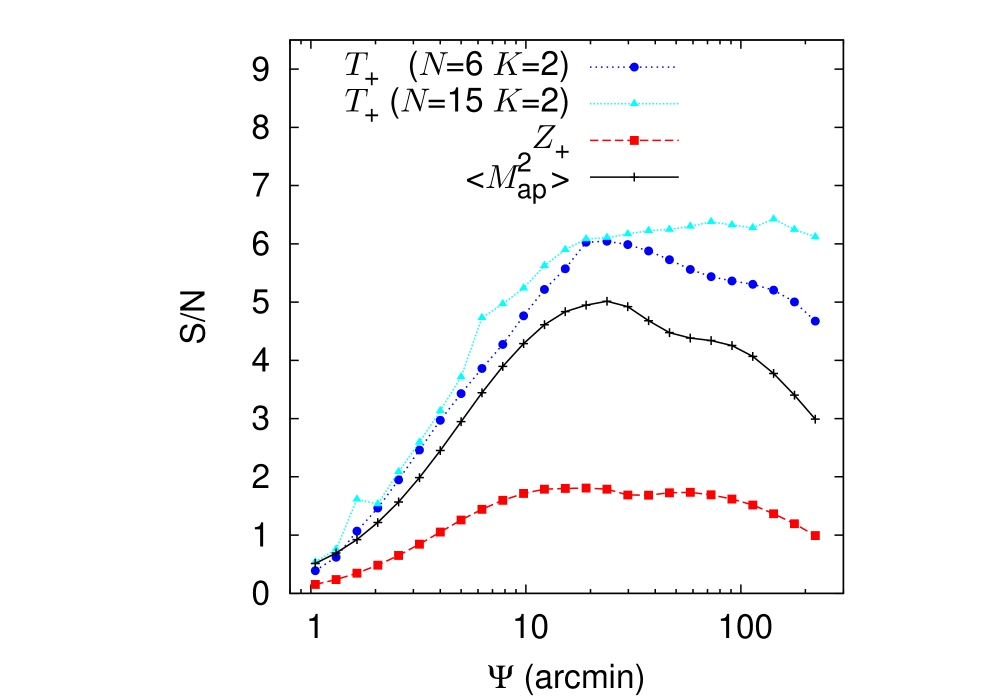
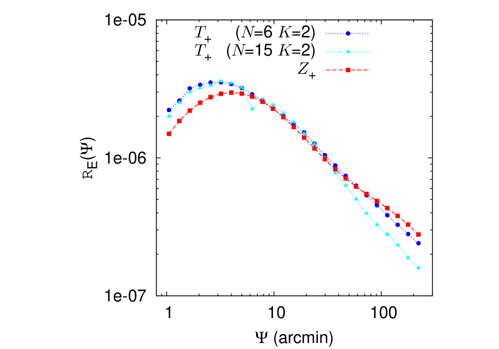
Figure 1: Left panel: Signal-to-noise ratio for fixed $\vartheta_{\rm min}=0.2\arcmin$, as functions of the maximum scale $\Psi$. The blue curve with circles and the cyan with triangles correspond to polynomial order $N=6$ and $N=15$, respectively. The red curve with squares shows the filter function from SK07. The black curve with crosses corresponds to the aperture-mass $\langle M_{\rm ap}^{2}\rangle$ with $\Psi$ being equal to the aperture diameter. Right panel: The comparison of ${\cal R}_{\rm E}$ obtained from the optimised function $T_{+}$ with polynomial orders $N=6$ and 15.

2.7 Optimisation

The maximisation of a quantity $Q$, to be defined in the next section as signal-to-noise ratio and Fisher matrix figure of merit, is done as follows. For a given polynomial order $N$ number of constraints $K\geq 2$, we perform the maximum search of $Q$ using the conjugate-gradient method Press et al. (1992) in the space of free coefficients $a_{K},\ldots,a_{N-1}$. At each step, we calculate $s_{m}$ (Eq. 19) and invert Eq. (20) to get the first $K$ coefficients $a_{0},\ldots a_{K-1}$; from there we compute $\tilde{T}_{+}$ (Eq. 14) and ${\cal R}_{\rm E}$ (Eq. 7).

We limit each of the coefficients $a_{K},\ldots,a_{N-1}$ to the box $[-10;10]$. In some cases the maximum-search fails, in particular if the polynomial order is high. The algorithm might run into a local maximum or hit the parameter boundary. To reduce the failure rate, we proceed as follows.

If a maximum is found close to the parameter boundary we discard it and redo the maximisation with larger box size for a different starting point. To initialise the maximisation for the first of a range of angular scales, we draw a number of random points, on the order 100, and start the maximisation with the point providing the largest $Q$.

For subsequent angular scales, we use the information about the previous maximum to start the next optimisation. If the ratio $\eta=\vartheta_{\rm min}/\vartheta_{\rm max}$ is kept constant when increasing $\vartheta_{\rm max}=\Psi$, we use the previous maximum coefficients $a_{n}$ as new starting value for the maximisation process. This renders the search for the maximum point more efficient and more stable, since for small changes in $\Psi$ the maximum will be close in $a$-space.

For constant minimum scale $\vartheta_{\rm min}$ we devise a different strategy. It can be shown that in this case, $Q$ is monotonously increasing with $\Psi$: Let $T_{+}^{(i)}$ be the function for scale $\Psi_{i}$ which maximises $Q(\Psi_{i})$. For the subsequent scale $\Psi_{i+1}>\Psi_{i}$, define the function $\bar{T}_{+}(\Psi)=T_{+}^{(i)}(\Psi)$ for $\Psi<\Psi_{i}$, and $\bar{T}_{+}(\Psi)=0$ otherwise. By construction, the resulting $Q$ for scale $\Psi_{i+1}$ is the same as for $\Psi_{i}$, $Q(\Psi_{i+1})=Q(\Psi_{i})$. Therefore, we choose as new starting point for scale $\Psi_{i+1}$ the coefficients resulting from the decomposition of the function $\bar{T}_{+}(\Psi)$. This assures the subsequent maximum $Q(\Psi_{i+1})$ found by the search algorithm to be larger or equal to the previous one, at least in the limit of large $N$. In practice however, due to the finite order $N$, the orthogonal polynomials are not a good representation of $\bar{T}_{+}$ for $\Psi>\Psi_{i}$ where it is zero, and the resulting $Q$ can actually decrease with increasing scale.

We summarise the the combinations of $Q$, the angular dependencies and the choice of the starting point for subsequent scales in Table 1.

Table 1: Overview of quantities kept fixed when varying the scales $\Psi$, and the corresponding method to determine the starting point for subsequent scales.

$Q$	Fixed quantity	Starting point for subsequent scales
S/N	$\vartheta_{\rm min}=\mbox{const.}$	Previous maximum function, $\bar{T}_{+}$
S/N	$\eta=\mbox{const.}$	Previous maximum coefficients $a_{n}$
FoM	$\eta=\mbox{const.}$	Previous maximum coefficients $a_{n}$

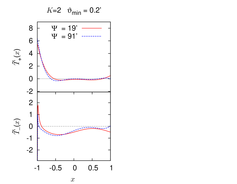
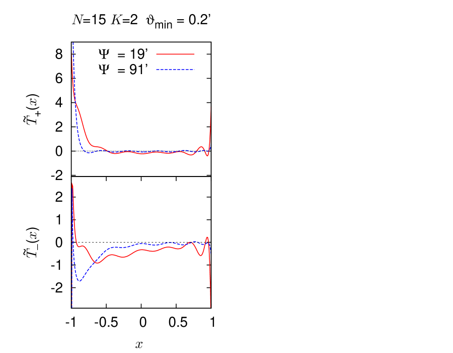
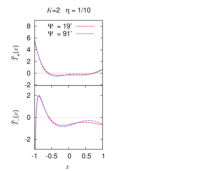
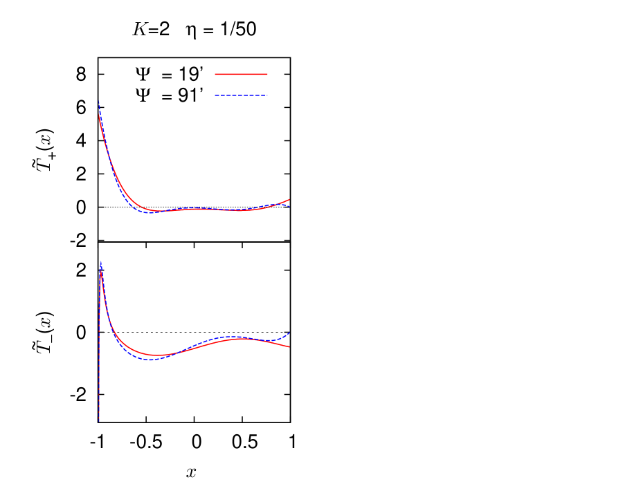
Figure 2: The normalised functions $\tilde{T}_{+}$ and $\tilde{T}_{-}$ optimised for signal-to-noise ratio at scales $\Psi=19\arcmin$ and $91\arcmin$, respectively. Left two panels: $\tilde{T}_{+}$ decomposed into polynomials of order $N=6$ and 15, respectively, for fixed $\vartheta_{\rm min}=0.2\arcmin$; Right two panels: The comparison of fixed $\eta=1/10$ and $1/50$ in the case of polynomials of order $N=6$.

3 Results

In this section we define $Q$ according to signal-to-noise and a Fisher-matrix figure of merit, respectively, which we maximise to find the corresponding optimised filter function $\tilde{T}_{+}$. Before that, we comment on our choice of $K$ and $N$, the number of constraints and polynomial order, respectively.

3.1 Number of constraints and polynomial order

We choose the minimum number of constraints $K=2$ necessary for a finite-interval E- and B-mode decomposition, corresponding to the two integral constraints (Eq. 9). Adding the two continuity constraints (Eq. 16) resulted in significantly lower values of $Q$. Some of the resulting functions $\tilde{T}_{\pm}$ showed strong variations and narrow peaks for $|x|$ near unity. This indicates that the continuity constraint is not very “natural” but represents a strong restriction on the optimised filter functions. The price that has to be paid for continuity is then a function which fluctuates strongly, which may be problematic when applied to noisy data.

Larger values of $N$ improved $Q$ to some extend but at the same time increased the occurrence of local maxima found by the search algorithm, reducing stability and reproducibility of the results. The functions $\tilde{T}_{\pm}$ sometimes showed a high number of oscillations. A good choice for the polynomial order $N$ was found to be 6, equivalent to 4 free parameters $a_{n}$ for $K=2$. A lower $N$ resulted in significantly smaller $Q$.

For the remainder of this paper we therefore choose $N=6$, $K=2$, if not indicated otherwise.

3.2 Shear covariance and cosmology

For the optimisation process we rely on a model shear correlation function and covariance. The fiducial cosmology for our model is a flat $\Lambda$CDM Universe with $\Omega_{\rm m}=0.25,\Omega_{\rm b}=0.044,h=0.7$ and $\sigma_{8}=0.8$. We use the non-linear fitting formula of Smith et al. (2003) together with the Eisenstein & Hu (1998) transfer function for the matter power spectrum. The redshift distribution of source galaxies is the best-fit model of Fu et al. (2008) which has a mean redshift of 0.95.

We use the covariance matrix $C_{++}$ of the shear correlation function $\xi_{+}$ from Fu et al. (2008), corresponding to the third data release of CFHTLS-Wide. This includes ellipticity noise and cosmic variance as well as the residual B-mode added in quadrature. The Gaussian part of the covariance was calculated using the method from Kilbinger & Schneider (2004). Non-Gaussian corrections on small scale were applied according to Semboloni et al. (2007).

The ${\cal R}_{\rm E}$-covariance matrix, $\langle{\cal R}_{\rm E}^{2}\rangle$, is an integral over $C_{++}$,

$$\left\langle{\cal R}_{\rm E}^{2}(\Psi_{1},\Psi_{2})\right\rangle=\int_{\vartheta_{{\rm min},1}}^{\Psi_{1}}{\mathrm{d}}\vartheta\,\vartheta T_{+}(\vartheta)\int_{\vartheta_{{\rm min},2}}^{\Psi_{2}}{\mathrm{d}}\vartheta^{\prime}\,\vartheta^{\prime}T_{+}(\vartheta^{\prime})C_{++}(\vartheta,\vartheta^{\prime}).$$ (36)

We use the two upper scale limits $\Psi_{1}$ and $\Psi_{2}$ as arguments of $\langle{\cal R}_{\rm E}^{2}\rangle$; it also depends on the two lower scale limits $\vartheta_{{\rm min},1}$ and $\vartheta_{{\rm min},2}$.

3.3 Signal-to-noise ratio

The first criterion for which we optimise the filter function is the signal-to-noise ratio

$$\rm{S/N}(\Psi)=\frac{{\cal R}_{\rm E}(\Psi)}{\left\langle{\cal R}_{\rm E}^{2}(\Psi,\Psi)\right\rangle^{1/2}}.$$ (37)

The variance $\langle{{\cal R}_{\rm E}^{2}(\Psi,\Psi)}\rangle$ is the diagonal of Eq. (36). As mentioned before, the signal-to-noise ratio does not depend on the normalisation of $\tilde{T}_{+}$ (Eq. 21).

3.3.1 Signal-to-noise for fixed $\vartheta_{\rm min}$

The signal-to-noise is calculated as a function of $\Psi=\vartheta_{\rm max}$, keeping $\vartheta_{\rm min}$ constant. We choose $\vartheta_{\rm min}=0.2\arcmin$ which is a typical (albeit conservative) lower limit where galaxies from ground-based data can be well separated. For each scale $\Psi$ we obtain an optimised filter function $T_{+}$, as discussed in Sect. 2.7 (see Table 1).

As can be seen in the left panel of Fig. 1 the optimal filter function with $N=6$ and $K=2$ results in a much higher signal-to-noise than for original ring statistic function $\langle{\cal RR}\rangle_{\rm E}$, using the filter function $Z_{+}$ from SK07. The new filter is superior to the aperture-mass dispersion. Note that we plot S/N for $\langle M_{\rm ap}^{2}\rangle$ as function of the aperture diameter instead of the radius, to have the same maximum shear correlation scale $\Psi$ as for ${\cal R}_{\rm E}$.

Although the optimal signal-to-noise is expected to be monotonic as function of $\Psi$, this is clearly not the case. However, when increasing the polynomial order $N$ to 15, the signal-to-noise is nearly constant for $\Psi>19\arcmin$ and larger than for $N=6$ (see Fig. 1). As a drawback, the S/N-curve for $N=15$ is less smooth due to the difficulty of finding the global maximum. We did in general not find significantly larger values for S/N with $N$ larger than 15.

The similar shape of S/N for the different cases ${\cal R}_{\rm E}$, $\langle M_{\rm ap}^{2}\rangle$ and $\langle{\cal RR}\rangle_{\rm E}$ is an imprint of the covariance structure of the shear correlation function. The shape is modified stronger for high $N$, where the peak at around 20 arc minutes disappears.

The shear function ${\cal R}_{\rm E}$ is plotted in the right panel of Fig. 1. It has a similar shape as $\langle{\cal RR}\rangle_{\rm E}$ from SK07, and also as $\langle M_{\rm ap}^{2}\rangle$. This is reflecting the fact that all functions correspond to narrow filters and are band-pass convolution of the power spectrum.

The normalised optimal filter functions for two angular scales are shown in the left two panels of Fig. 2. The similarity of the functions for different scales shows the relatively weak dependence of the filter shape on angular scale.

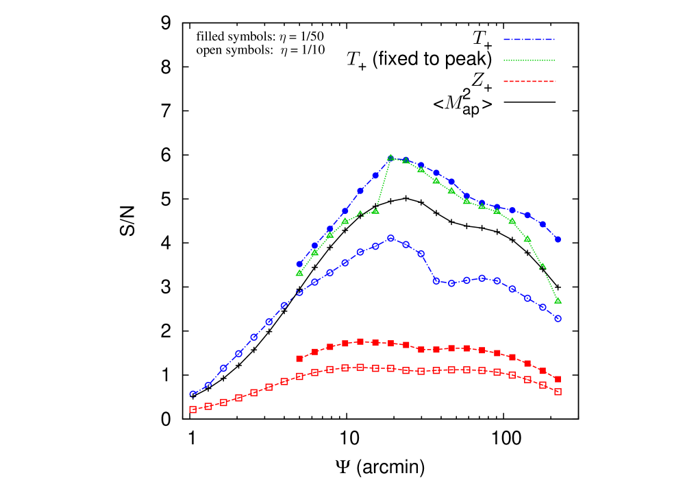
Figure 3: Left panel: Signal-to-noise ratio as function of $\Psi$, for fixed values of $\eta$ with $N=6$ and $K=2$. The blue curves correspond to the optimised function $\tilde{T}_{+}$. The green curve is obtained by applying the the optimal function $T_{+}$ of $\Psi=19\arcmin$ to all scales, instead of optimising each time separately, as done for the blue lines. The red curves shows the filter function $Z_{+}$ from SK07. The black curve with crosses corresponds to the aperture-mass with aperture diameter $\vartheta_{\rm max}$. Filled and open symbols represent $\eta=1/50$ and $1/10$, respectively. Right panel: ${\cal R}_{\rm E}$ for fixed values of $\eta$ of $1/10$ (open circles) and 1/50 (filled). For the green line (with filled triangles), the optimal function $\tilde{T}_{+}$ for $\Psi=19\arcmin$ was used on all scales, instead of optimising each time separately as for the blue lines.

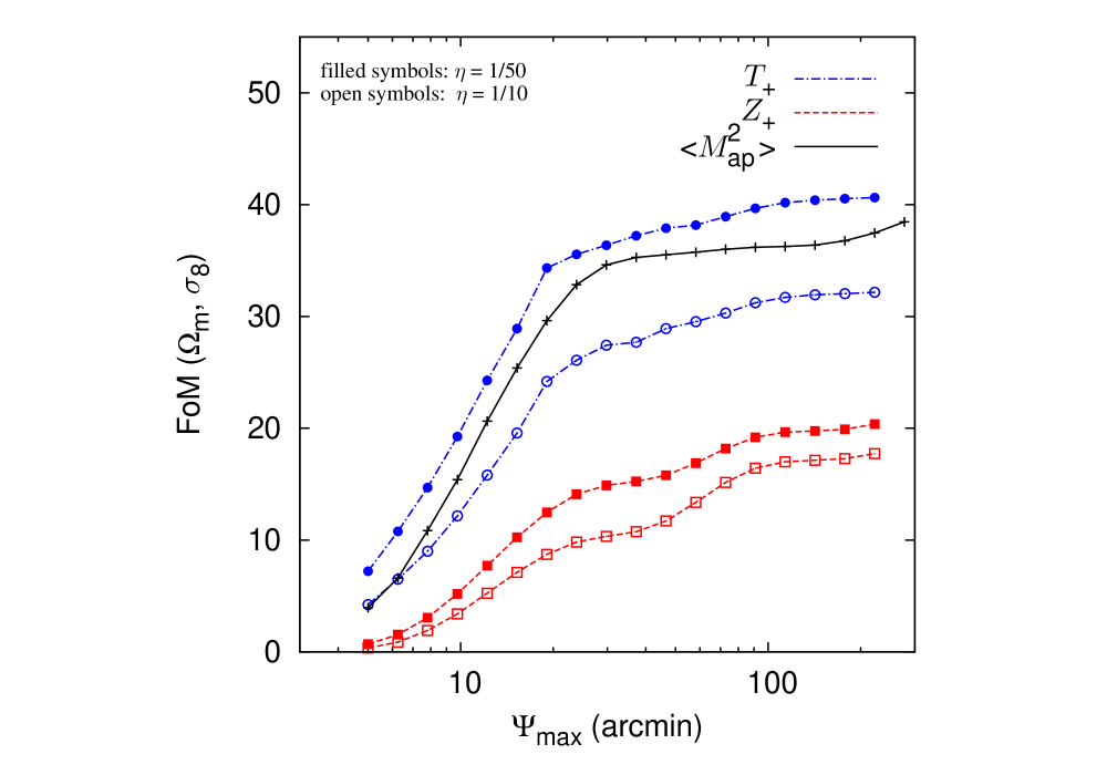
Figure 4: Figure of merit (FoM, Eq. 39) for the optimised filter function $T_{+}$ with $\eta=1/10$ and $\eta=1/50$ (blue curves). The red curves shows the FoM for the filter function $Z_{+}$ from SK07. The black curve with crosses corresponds to the aperture-mass with aperture diameter $\vartheta_{\rm max}$. Filled and open symbols represent $\eta=1/50$ and $1/10$, respectively.

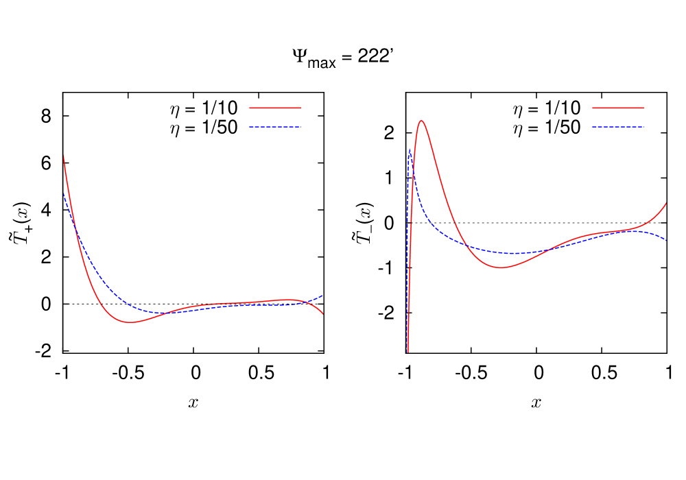
Figure 5: The normalised functions $\tilde{T}_{+}$ and $\tilde{T}_{-}$, optimised for the Fisher matrix figure of merit (Eq. 39) with $\Psi_{\rm max}=222\arcmin$. Two cases, $\eta=1/10$ and 1/50 are shown.

3.3.2 Signal-to-noise for fixed $\eta$

Instead of fixing $\vartheta_{\rm min}$, we now leave $\eta$ constant and change $\vartheta_{\rm min}$ along with $\Psi$. The signal-to-noise ratio increases with decreasing $\eta$ (left panel of Fig. 3). This is not surprising since a larger $\eta$ means a smaller range of angular scales. For $\eta=1/50$ the optimal S/N exceeds the one using the aperture-mass dispersion. The optimal filter functions have similar shape to the previous case of a fixed $\vartheta_{\rm min}$ (see the right two panels of Fig. 2). We use the previous maximum coefficients $a_{n}$ as starting point for subsequent scales as discussed in Sect. 2.7 (see Table 1). Unlike in the previous case of fixed $\vartheta_{\rm min}$ we do not expect S/N to be monotonous as function of $\Psi$, because $\vartheta_{\rm min}$ increases with $\Psi$.

Since $\eta$ is constant, each filter function provides a valid E-/B-mode decomposition for any given scale. We use the filter optimised for $\Psi=19\arcmin$, where the highest signal-to-noise occurs, and apply it to the other scales (see the green curve with triangles in the left panel of Fig. 3). As expected, the signal-to-noise for scales $\Psi\neq 19\arcmin$ is lower than in the previous case, where the optimisation was done for each scale individually. The difference however is not large and this case of fixed $\eta$ shows a S/N which is mostly larger than the aperture-mass dispersion.

The shear function ${\cal R}_{\rm E}$ is plotted in the right panel of Fig. 3, it is very similar in shape as in the case of fixed $\vartheta_{\rm min}$ (Sect. 3.3.1). Table 2 shows the polynomial coefficients of the corresponding filter function $\tilde{T}_{+}$.

3.4 Fisher matrix

Covariance matrix of ${\cal R}_{\rm E}$

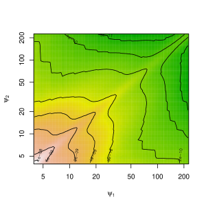
Correlation matrix of ${\cal R}_{\rm E}$

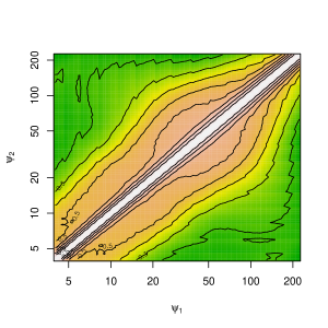
Covariance matrix of $\langle M_{\rm ap}^{2}\rangle$

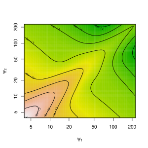
Correlation matrix of $\langle M_{\rm ap}^{2}\rangle$

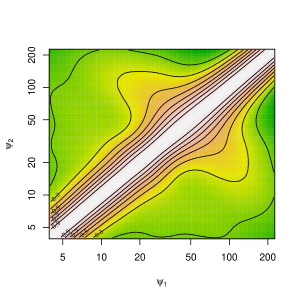
Figure 6: Covariance matrix (left panels) and correlation matrix (right) of ${\cal R}_{\rm E}$, optimised for the figure of merit (Eq. 39) with $\eta=1/50$ (top), and of the aperture-mass dispersion with $\Psi_{i}$ being equal to the aperture diameter (bottom). The colors correspond to the same levels for ${\cal R}_{\rm E}$ and $\langle M_{\rm ap}^{2}\rangle$. In the right panels, the contour lines start from the innermost value of 0.9 and are spaced by 0.1.

To optimise the filter function we take now the alternative approach of minimising the errors on cosmological parameters from our new second-order shear statistic. To that end, we use the Fisher matrix $F$, given by

$$F_{\alpha\beta}=\sum_{ij}\left\langle{\cal R}_{\rm E}^{2}(\Psi_{i},\Psi_{j})\right\rangle^{-1}\frac{\partial{\cal R}_{\rm E}(\Psi_{i})}{\partial p_{\alpha}}\frac{\partial{\cal R}_{\rm E}(\Psi_{j})}{\partial p_{\beta}}.$$ (38)

The cosmological parameters are comprised in the vector $\boldsymbol{p}$. As in the case of the signal-to-noise ratio, the Fisher matrix is independent of the normalisation of the filter function $\tilde{T}_{+}$.

The quantity $Q$ to be maximised is the inverse area of the error ellipsoid in parameter space, given by the Fisher matrix. In two dimensions this figure of merit (FoM, Albrecht et al. 2006) is

$${\rm FoM}^{-1}=\pi\left(\sigma_{11}\sigma_{22}-\sigma_{12}^{2}\right)^{1/2};\;\;\;\;\sigma_{ij}^{2}=\left(F^{-1}\right)_{ij}.$$ (39)

Eifler, Schneider & Krause (2009) used the quadrupole moment determinant $q$ of the likelihood function to quantify the size of the parameter confidence region. In case of a Gaussian likelihood (which correspond to our Fisher matrix approximation) in two dimensions, the relation FoM${}^{-1}=\pi q$ holds.

We keep $\eta$ constant, allowing for a single filter function $\tilde{T}_{+}$ to provide the E- and B-mode decomposition for each scale $\Psi$ in Eq. (38), and also for the covariance matrix. This requirement is not a necessity since the covariance between scales can be easily generalised to different filter functions. However, we choose this approach for simplicity. The cosmological parameters we consider are $\Omega_{\rm m}$ and $\sigma_{8}$.

In Fig. 4 we compare the figure of merit for the optimised filter function and the aperture-mass dispersion. For a given maximum scale $\Psi_{\rm max}$ we vary $\Psi_{i}$ in Eq. (38) between $4.0\arcmin$ and $\Psi_{\rm max}$. With $\eta=1/50$, the minimum angular scale is ${\min}(\vartheta_{\rm min})=4.8$ arc second. For $\eta=1/10$ we use the same angular scales, starting with 4.0′, for consistency with the case $\eta=1/50$. Alternatively, by using the same minimum angular scale of 4.8 arc second, the smallest $\Psi$ can be in principle as small as $4.8\arcsec/\eta=0.8\arcmin$. This addition of small scales results in a higher FoM which is comparable to the one for $\langle M_{\rm ap}^{2}\rangle$.

We choose the same range of scales for the aperture-mass dispersion, i.e. we vary the aperture diameter between $4.0\arcmin$ and $\Psi_{\rm max}$. Note that although the minimum angular scale is theoretically zero, in practise we are limited by the smallest scale for which the $\xi_{+}$-covariance matrix is calculated which is $3\arcsec$ in our case.

The normalised optimal filter functions $\tilde{T}_{\pm}$ are shown in Fig. 5. They have a similar shape as the functions optimised for S/N (see Fig. 2). Table 2 shows the corresponding polynomial coefficients.

3.5 The covariance of ${\cal R}_{\rm E}$

We calculate the covariance matrix $C$ of ${\cal R}_{\rm E}$ using the optimal filter function from the figure-of-merit maximisation at the largest scale $\Psi_{\rm max}=222\arcmin$, for a constant $\eta=1/50$, see Sect. 3.4. As can be seen in Fig. 6 the covariance is diagonally-dominated, similar to the one of the aperture-mass dispersion. The degree of correlation is seen more clearly by regarding the correlation matrix

$$r(\Psi_{1},\Psi_{2})=\frac{\langle{\cal R}_{\rm E}^{2}(\Psi_{1},\Psi_{2})\rangle}{\langle{\cal R}_{\rm E}^{2}(\Psi_{1},\Psi_{1})\rangle\langle{\cal R}_{\rm E}^{2}(\Psi_{2},\Psi_{2})\rangle},$$ (40)

see the right panels of Fig. 6. To quantify the correlation length, we compute the following function,

$$\tau(x)=\left\langle r(\Psi,x\Psi)\right\rangle_{\Psi},$$ (41)

which is the correlation between two scales separated by the multiplicative factor $x$, averaged over all $\Psi$. This function is shown in Fig. 7. Since the lines of equal $r$ are mainly parallel to the diagonal, the scatter is relatively small. The correlation of ${\cal R}_{\rm E}$ drops off faster near the diagonal than the one for $\langle M_{\rm ap}^{2}\rangle$, and shows a slightly larger correlation at intermediate distances $x$. The covariance of $\langle{\cal RR}\rangle_{\rm E}$ has been studied in Eifler, Schneider & Krause (2009) and has significantly smaller correlation length than the one for $\langle M_{\rm ap}^{2}\rangle$.

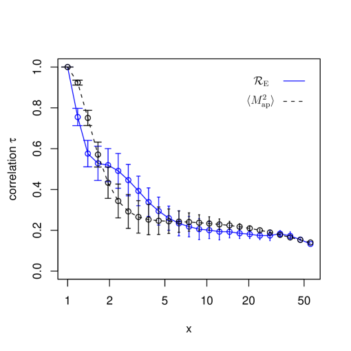
Figure 7: The average correlation $\tau$ (Eq. 41) for scales which are separated by the ratio $x$, for ${\cal R}_{\rm E}$ (solid, blue lines) and $\langle M_{\rm ap}^{2}\rangle$ (dashed, black curve). The error bars indicate the scatter when averaging over different scales $\Psi$.

3.6 Numerical limits on the B-mode ${\cal R}_{\rm B}$

We calculate the B-mode ${\cal R}_{\rm B}$ from Eq. (1) by using $\tilde{T}_{-}$ obtained from the optimal function $\tilde{T}_{+}$ (see Sect. 2.4). Theoretically, ${\cal R}_{\rm B}$ vanishes but there could be a residual B-mode because the E-/B-mode decomposition might not be perfect. For example, there could be numerical issues regarding the matrix inversion of Eq. (20). Our values of ${\cal R}_{\rm B}$ are limited by the precision of the numerical integration of Eq. (1). ${\cal R}_{\rm B}$ goes to zero for decreasing integration step size and we did not find evidence for a residual B-mode. For a step size of $\Delta\vartheta=5\cdot 10^{-4}$ arc seconds, we find ${\cal R}_{\rm B}/{\cal R}_{\rm E}<2\cdot 10^{-5}$ for all angular scales. Even if a residual B-mode should be present, it is straightforward to make it vanish identically. One can increase the polynomial order $N$ of the decomposition by one, and determine the corresponding coefficient $a_{N-1}$ such that ${\cal R}_{\rm B}=0$.

Table 2: Coefficients $a_{n}$ of the optimised function $\tilde{T}_{+}$ for (1) S/N, $\Psi=19\arcmin,\eta=1/50$; (2) FoM, $\Psi_{\rm max}=222\arcmin,\eta=1/10$; (3) FoM, $\Psi_{\rm max}=222\arcmin,\eta=1/50$.

	$\phantom{-}\rm{S/N}$ ($\Psi=19\arcmin$)	FoM ($\Psi=222\arcmin$)
$n$	$\phantom{-}a_{n}$ $(\eta=1/50)$	$\phantom{-}a_{n}$ $(\eta=1/10)$	$\phantom{-}a_{n}$ $(\eta=1/50)$
0	$\phantom{-}0.1197730890$	$\phantom{-}0.009877788826$	$\phantom{-}0.1239456383$
1	$-0.3881211865$	$\phantom{-}0.1061397843$	$-0.3881431858$
2	$\phantom{-}0.5212557875$	$-0.4300211814$	$\phantom{-}0.5579593467$
3	$-0.3440507036$	$\phantom{-}0.5451016406$	$-0.3679282338$
4	$\phantom{-}0.2761305382$	$-0.3372272549$	$\phantom{-}0.1540941993$
5	$-0.07286690971$	$\phantom{-}0.1716983151$	$\phantom{-}0.01293361618$

3.7 Dependence on cosmology and survey parameters

The results presented in this paper have been obtained by using a specific covariance matrix of $C_{++}$, namely the one used in Fu et al. (2008), and by choosing a specific cosmology. Here, we briefly describe how our results change when we modify these parameters.

First, we illustrate the dependence on the covariance matrix. Instead of using the full covariance, as was done in the previous sections, we repeat the S/N-analysis by taking the diagonal shot-noise component only. This noise origins from the intrinsic galaxy ellipticity dispersion. As expected, the S/N and FoM increase substantially, mainly because of the missing cross-correlation between angular scales in the shear correlation function. For all three cases, ${\cal R}_{\rm E},\langle M_{\rm ap}^{2}\rangle$ and $\langle{\cal RR}\rangle_{\rm E}$, the S/N increases monotonously with $\Psi$ beyond the maximum scale and does not show a peak at around 20 arc minutes. The relative trend between the three cases stays the same.

We change the fiducial cosmological model by increasing $\sigma_{8}$ from 0.8 to 0.9. This results in an increase of S/N of a factor between 1.3 and 1.4, which is roughly the same for ${\cal R}_{\rm E},\langle M_{\rm ap}^{2}\rangle$ and $\langle{\cal RR}\rangle_{\rm E}$. Increasing the mean redshift from 0.95 to 1.19 caused the S/N to be higher by 1.8 to 2, in the same way for all three cases. We conclude that the relative difference is not dependent on cosmology or the redshift distribution.

We repeat the calculation of S/N by choosing a fixed $\vartheta_{\rm min}$ which is different from our standard value of 0.2 arc minutes. The improvement of ${\cal R}_{\rm E}$ over $\langle{\cal RR}\rangle_{\rm E}$ decreases for decreasing $\vartheta_{\rm min}$, by about $\Delta$(S/N) = 0.1 for $\Delta\vartheta_{\rm min}=0.1\arcmin$, averaged over all scales $\Psi$. This might be because $\langle{\cal RR}\rangle_{\rm E}$ shows less cross-correlation between scales which leads to a larger gain when additional scales are included. The gain of ${\cal R}_{\rm E}$ with respect to $\langle M_{\rm ap}^{2}\rangle$ increases when lowering $\vartheta_{\rm min}$, as expected, since the inclusion of more small scales boosts the S/N. On average, the difference is 0.05 for each 0.1 arc minute which leads to an asymptotic value of [S/N(${\cal R}_{\rm E}$)]/[S/N($\langle M_{\rm ap}^{2}\rangle$)] = 1.31.

To check the stability of the results, we add an independent, uniform random variable between $-p$ and $p$ to each of the highest $N-K$ coefficients $a_{n}$ after the optimum has been found. For each randomisation we fix $a_{0},\ldots,a_{K-1}$ as described in Sect. 2.3 to assure E-/B-mode separation. The S/N and FoM are very robust against changes in the coefficients. For both $p=0.01$ and 0.1, the changes in S/N and FoM are on the order $p$ and less.

4 Summary

We have introduced a new second-order cosmic shear function which has the ability to separate E- and B-modes on a finite interval of angular scales. This function is a generalisation of the recently introduced “ring statistic” (SK07). Providing the second-order E-/B-mode shear field correlations, general filter functions are calculated and optimised for a specific goal. In this paper, we considered the signal-to-noise ratio (S/N) as function of angular scale, and a figure of merit (FoM) based on the Fisher matrix of the cosmological parameters $\Omega_{\rm m}$ and $\sigma_{8}$ as optimisation criteria.

Our method to find the optimal filter function consists in the following steps:

1. Choose the polynomial order $N$ and number of constraints $K\geq 2$ and define a quantity $Q$ to be maximised (in this work the signal-to-noise ratio S/N and the Fisher matrix figure-of-merit FoM).

2. Draw a random starting vector of coefficients $a_{K},\ldots a_{N-1}$.

3. For $m=0\ldots K-1$ calculate $s_{m}$ (Eq. 19).

4. Invert the constraints matrix equation (20) to get the first $K$ coefficients $a_{0}\ldots a_{K-1}$.

5. Compute the filter function $T_{+}$ (Eqs. 11, 14)

6. Calculate the shear function ${\cal R}_{\rm E}$ (Eq. 7) and $Q$ (in this work Eqs. 37, 38).

7. Maximise $Q$. At each iteration of the maximisation process, repeat steps 3.-6.

We were able to improve both S/N and FoM substantially with respect to the SK07 ring statistic. Moreover, we obtained better results than for the aperture-mass dispersion $\langle M_{\rm ap}^{2}\rangle$, even though the latter formally extends to zero lag and includes therefore more small-scale power.

We have adapted and optimised our new second-order statistic ${\cal R}_{\rm E}$ to a specific cosmology and survey parameters such as area and depth. We used a smallest scale of 0.2′which corresponds to the smallest separation for which galaxy images can easily be separated using ground-based imaging data. The cosmic shear-correlation covariance corresponds to the CFHTLS-Wide third data release used for weak cosmological lensing (Fu et al. 2008). The coefficients corresponding to the optimal filter functions can be found in Table 2. A C-program which calculates the filter functions and the shear statistic ${\cal R}_{\rm E}$ is freely available.

Our specific results can be applied to other requirements, although the results will not be optimal. Alternatively, the optimisation method described here can easily be applied to any given survey setting. For space-based surveys, where the galaxy-blending confusion limit is smaller than for ground-based observations, the advantage of ${\cal R}_{\rm E}$ over $\langle M_{\rm ap}^{2}\rangle$ is more pronounced.

5 Outlook

The new cosmic shear functions ${\cal R}_{\rm E}$ and ${\cal R}_{\rm B}$ can be applied in various ways in the context of detecting systematics in cosmic shear data and for constraining cosmological parameters.

The optimisation for signal-to-noise is useful for detecting a potential B-mode in the data. In this case the E-/B-mode decomposition serves merely as a diagnostic of the observations. A significant B-mode can be a sign for residuals in the PSF correction or non-perfect shape measurement. It might also hint to an astrophysically generated B-mode signal, for example from shape-shear correlations or shape-shape intrinsic alignment. In both cases, the B-mode signal is expected to be small and it is of great importance to obtain a clear E-/B-mode separation without mixing of modes.

In case of a suspected astrophysical B-mode, the separation of the shear field into E- and B-modes might be a decisive advantage. If the power spectrum contains both an E- and B-mode, $P_{\rm tot}=P_{\rm E}+P_{\rm B}$, both modes mix together into their Fourier-transform of $P_{\rm tot}$, the shear correlation function. Thus, the E- and B-mode may not be uniquely reconstructed from the correlation functions. The different astrophysical components giving rise to $P_{\rm E}$ and $P_{\rm B}$ can then only be separated by a E-/B-mode separating filter.

The figure-of-merit optimisation permits ${\cal R}_{\rm E}$ to be used for efficient constraints on cosmological parameters. The reason to use a filtered version of the shear correlation function $\xi_{\pm}$ instead of the latter directly can be manifold (Eifler et al. 2008). A filter can be chosen to be a narrow pass-band filter of the power spectrum and is therefore able to probe its local features, unlike the broad low-pass band function $\xi_{+}$. As a consequence, the correlation length is much smaller and the covariance matrix close to diagonal. This has numerical advantages in particular in the case of many data points, e.g. for shear tomography. Finally, higher-order moments (skewness, kurtosis, $\ldots$) of filtered quantities are easier to handle than higher-order statistics of the (spin-2) shear field (Jarvis et al. 2004; Schneider et al. 2005).

Apart from S/N and FoM maximisation, one can think of other, alternative quantities with respect to which the filter function can be optimised. For example, if a model for the B-mode is assumed, the signal-to-noise of ${\cal R}_{\rm B}$ can be optimised to facilitate the possible detection of a B-mode. Further, if cosmic shear is combined with other probes of cosmology; the relative gain from weak lensing could be maximised. This can be done for specific goals, for example a given dark-energy parametrisation or some alternative theory of modified gravity. However, we emphasis that the possibilities are restricted since the optimisation is always limited by the information contained in the lensing power spectrum.

In the case of shear tomography, where the shear signal from different redshifts is resolved (although only partially due to the broad lensing efficiency kernel), one can perform a redshift-dependent optimisation of the filter function. This is expected to bring further improvements: Firstly, the projection of physical onto angular scales varies with redshift; using a redshift-dependent filter function, physical scales can be sampled optimally with redshift. Secondly, the power spectrum changes with varying redshift; to optimise the sampling of this redshift-dependent information might require a redshift-varying filter.

${\cal R}_{\rm E}$ is beneficial in particular on small scales, where the aperture-mass dispersion suffers from mode-mixing. On scales less than a few arc minutes there is a leakage of modes of about 10% (Kilbinger et al. 2006). Those scales contain information about halo structure, substructure and baryonic physics. It is difficult to model those effects, the use of those small scales to constrain cosmological parameters is limited. On the other hand, lensing observations on small scales will provide important constraints on the physical processes involved and matter properties on small scales.

Appendix A Simultaneous optimisation for arbitrary scales

The optimisation scheme introduced in this paper holds for a given ratio of minimum and maximum scale $\eta=\vartheta_{\rm min}/\vartheta_{\rm max}$. In this section we introduce a simple generalisation of the scheme to obtain an optimised function $\tilde{T}_{+}$ which fulfills the integral constraints (Eq. 9) for all $(\vartheta_{\rm min},\vartheta_{\rm max})$. This comes at the expense of a poor resulting signal-to-noise.

If we demand the following relation to hold

$$I_{\nu}\equiv\int_{-1}^{+1}{\mathrm{d}}x\,x^{\nu}\tilde{T}_{+}(x)=0;\;\;\;\;\mbox{for}\;\;\;\;\nu=0,1,2,3,$$ (42)

then the two integral constraints

$$RI_{0}+I_{1}=R^{3}I_{0}+R^{2}I_{1}+RI_{2}+I_{3}=0$$ (43)

are satisfied. However, instead of two conditions we have now four equations (Eq. 42) which fix $K=4$ coefficients of the decomposition. In this case, the first four matrix elements are (cf. Eq. 17)

$$f_{mn}=\int_{-1}^{+1}{\mathrm{d}}x\,x^{m}\,C_{n}(x);\;\;\;\;m=0\ldots 3.$$ (44)

Since there are two more integrals than in the previous case, the resulting function has at least two more zeros. The corresponding signal-to-noise ratio is significantly lower than in the single-scale case; it is even smaller than the one obtained for $Z_{+}$. We therefore do not consider this option further.

References

- Albrecht et al. (2006) Albrecht A., Bernstein G., Cahn R., Freedman W. L., Hewitt J., Hu W., Huth J., Kamionkowski M., Kolb E. W., Knox L., Mather J. C., Staggs S., Suntzeff N. B., 2006
- Benjamin et al. (2007) Benjamin J., Heymans C., Semboloni E., Van Waerbeke L., Hoekstra H., Erben T., Gladders M. D., Hetterscheidt M., Mellier Y., Yee H. K. C., 2007, \mnras, 381, 702
- Crittenden et al. (2002) Crittenden R. G., Natarajan P., Pen U.-L., Theuns T., 2002, \apj, 568, 20
- Eifler et al. (2008) Eifler T., Kilbinger M., Schneider P., 2008, \aap, 482, 9