Search-based Structured Prediction

Abstract

We present Searn, an algorithm for integrating search and learning to solve complex structured prediction problems such as those that occur in natural language, speech, computational biology, and vision. Searn is a meta-algorithm that transforms these complex problems into simple classification problems to which any binary classifier may be applied. Unlike current algorithms for structured learning that require decomposition of both the loss function and the feature functions over the predicted structure, Searn is able to learn prediction functions for any loss function and any class of features. Moreover, Searn comes with a strong, natural theoretical guarantee: good performance on the derived classification problems implies good performance on the structured prediction problem.

1 Introduction

Prediction is the task of learning a function $f$ that maps inputs $x$ in an input domain $\mathcal{X}$ to outputs $y$ in an output domain $\mathcal{Y}$. Standard algorithms—support vector machines, decision trees, neural networks, etc.—focus on “simple” output domains such as $\mathcal{Y}=\{-1,+1\}$ (in the case of binary classification) or $\mathcal{Y}=\mathbb{R}$ (in the case of univariate regression).

We are interested in problems for which elements $y\in\mathcal{Y}$ have complex internal structure. The simplest and best studied such output domain is that of labeled sequences. However, we are interested in even more complex domains, such as the space of English sentences (for instance in a machine translation application), the space of short documents (perhaps in an automatic document summarization application), or the space of possible assignments of elements in a database (in an information extraction/data mining application). The structured complexity of features and loss functions in these problems significantly exceeds that of sequence labeling problems.

From a high level, there are four dimensions along which structured prediction algorithms vary: structure (varieties of structure for which efficient learning is possible), loss (different loss functions for which learning is possible), features (generality of feature functions for which learning is possible) and data (ability of algorithm to cope with imperfect data sources such as missing data, etc.). An in-depth discussion of alternative structured prediction algorithms is given in Section 5. However, to give a flavor, the popular conditional random field algorithm lafferty01crf is viewed along these dimensions as follows. Structure: inference for a CRF is tractable for any graphical model with bounded tree width; Loss: the CRF typically optimizes a log-loss approximation to 0/1 loss over the entire structure; Features: any feature of the input is possible but only output features that obey the graphical model structure are allowed; Data: EM can cope with hidden variables.

We prefer a structured prediction algorithm that is not limited to models with bounded treewidth, is applicable to any loss function, can handle arbitrary features and can cope with imperfect data. Somewhat surprisingly, Searn meets nearly all of these requirements by transforming structured prediction problems into binary prediction problems to which a vanilla binary classifier can be applied. Searn comes with a strong theoretical guarantee: good binary classification performance implies good structured prediction performance. Simple applications of Searn to standard structured prediction problems yield tractable state-of-the-art performance. Moreover, we can apply Searn to more complex, non-standard structured prediction problems and achieve excellent empirical performance.

This paper has the following outline:

1. Introduction.

2. Core Definitions.

3. The Searn Algorithm.

4. Theoretical Analysis.

5. A Comparison to Alternative Techniques.

6. Experimental results.

7. Discussion.

2 Core Definitions

In order to proceed, it is useful to formally define a structured prediction problem in terms of a state space.

Definition 1

A structured prediction problem $\mathcal{D}$ is a cost-sensitive classification problem where $\mathcal{Y}$ has structure: elements $y\in\mathcal{Y}$ decompose into variable-length vectors $(y_{1},y_{2},\dots,y_{T})$. $\mathcal{D}$ is a distribution over inputs $x\in\mathcal{X}$ and cost vectors $\boldsymbol{c}$, where $\left|\boldsymbol{c}\right|$ is a variable in $2^{T}$.

As a simple example, consider a parsing problem under F${}_{1}$ loss. In this case, $\mathcal{D}$ is a distribution over $(x,\boldsymbol{c})$ where $x$ is an input sequence and for all trees $y$ with $\left|x\right|$-many leaves, $c_{y}$ is the F${}_{1}$ loss of $y$ on the “true” output.

The goal of structured prediction is to find a function $h:\mathcal{X}\rightarrow\mathcal{Y}$ that minimizes the loss given in Eq (1).

$$L(\mathcal{D},h)=\mathbb{E}_{(x,\boldsymbol{c})\sim\mathcal{D}}\left\{c_{h(x)}\right\}$$ (1)

The algorithm we present is based on the view that a vector $y\in\mathcal{Y}$ can be produced by predicting each component $(y_{1},\dots,y_{T})$ in turn, allowing for dependent predictions. This is important for coping with general loss functions. For a data set $(x_{1},c_{1}),\dots,(x_{N},c_{N})$ of structured prediction examples, we write $T_{n}$ for the length of the longest search path on example $n$, and $T_{\textrm{max}}=\max_{n}T_{n}$.

3 The Searn Algorithm

There are several vital ingredients in any application of Searn: a seach space for decomposing the prediction problem; a cost sensitive learning algorithm; labeled structured prediction training data; a known loss function for the structured prediction problem; and a good initial policy. These aspects are described in more detail below.

A search space $\mathcal{S}$.

The choice of search space plays a role similar to the choice of structured decomposition in other algorithms. Final elements of the search space can always be referenced by a sequence of choices $\hat{\boldsymbol{y}}$. In simple applications of Searn the search space is concrete. For example, it might consist of the parts of speech of each individual word in a sentence. In general, the search space can be abstract, and we show this can be beneficial experimentally. An abstract search space comes with an (unlearned) function $f(\hat{\boldsymbol{y}})$ which turns any sequence of predictions in the abstract search space into an output of the correct form. (For a concrete search space, $f$ is just the identity function. To minimize confusion, we will leave off $f$ in future notation unless its presence is specifically important.)

A cost sensitive learning algorithm $A$.

The learning algorithm returns a multiclass classifier $h(s)$ given cost sensitive training data. Here $s$ is a description of the location in the search space. A reduction of cost sensitive classification to binary classification beygelzimer05reductions reduces the requirement to a binary learning algorithm. Searn relies upon this learning algorithm to form good generalizations. Nothing else in the Searn algorithm attempts to achieve generalization or estimation. The performance of Searn is strongly dependent upon how capable the learned classifier is. We call the learned classifier a policy because it is used multiple times on inputs which it effects, just as in reinforcement learning.

Labeled structured prediction training data.

Searn digests the labeled training data for the structured prediciton problem into cost-sensitive training data which is fed into the cost-sensitive learning algorithm.

A known loss function.

A loss function $L(\boldsymbol{y},f(\hat{\boldsymbol{y}}))$ must be known and be computable for any sequence of predictions.

A good initial policy.

This policy should achieve low loss when applied to the training data. This can (but need not always) be defined using a search algorithm.

3.1 Searn at Test Time

Searn at test time is a very simple algorithm. It uses the policy returned by the learning algorithm to construct a sequence of decisions $\hat{\boldsymbol{y}}$ and makes a final prediction $f(\hat{\boldsymbol{y}})$. First, one uses the learned policy to compute $y_{0}$ on the basis of just the input $x$. One then computes $y_{1}$ on the basis of $x$ and $y_{0}$, followed by predicting $y_{2}$ on the basis of $x$, $y_{0}$ and $y_{1}$, etc. Finally, one predicts $y_{T}$ on the basis of the input $x$ and all previous decisions.

3.2 Searn at Train Time

Searn operates in an iterative fashion. At each iteration it uses a known policy to create new cost-sensitive classification examples. These examples are essentially the classification decisions that a policy would need to get right in order to perform search well. These are used to learn a new classifier, which is interpreted as a new policy. This new policy is interpolated with the old policy and the process repeats.

3.2.1 Initial Policy

Searn relies on a good initial policy on the training data. This policy can take full advantage of the training data labels. The initial policy needs to be efficiently computable for Searn to be efficient. The implications of this assumption are discussed in detail in Section 3.4.1, but it is strictly weaker than assumptions made by other structured prediction techniques. The initial policy we use is a policy that, for a given state predicts the best action to take with respect to the labels:

Definition 2 (Initial Policy)

For an input $x$ and a cost vector $\boldsymbol{c}$ as in Def 1, and a state $s=x\times(y_{1},\dots,y_{t})$ in the search space, the initial policy $\pi(s,\boldsymbol{c})$ is $\arg\min_{y_{t+1}}\min_{y_{t+2},\dots,y_{T}}c_{\langle y_{1},\dots,y_{T}\rangle}$. That is, $\pi$ chooses the action (i.e., value for $y_{t+1}$) that minimizes the corresponding cost, assuming that all future decisions are also made optimally.

This choice of initial policy is optimal when the correct output is a deterministic function of the input features (effectively in a noise-free environment).

3.2.2 Cost-sensitive Examples

In the training phase, Searn uses a given policy $h$ (initialized to the the initial policy $\pi$) to construct cost-sensitive multiclass classification examples from which a new classifier is learned. These classification examples are created by running the given policy $h$ over the training data. This generates one path per structured training example. Searn creates a single cost-sensitive example for each state on each path. The classes associated with each example are the available actions (or next states). The only difficulty lies in specifying the costs.

The cost associated with taking an action that leads to state $s$ is the regret associated with this action, given our current policy. For each state $s$ and each action $a$, we take action $a$ and then execute the policy to gain a full sequence of predictions $\hat{\boldsymbol{y}}$ for which we can compute a loss $\boldsymbol{c}_{\hat{\boldsymbol{y}}}$. Of all the possible actions, one, $a^{\prime}$, has the minimum expected loss. The cost $\ell_{h}(\boldsymbol{c},s,a)$ for an action $a$ in state $s$ is the difference in loss between taking action $a$ and taking the action $a^{\prime}$; see Eq (2).

$$\ell_{h}(\boldsymbol{c},s,a)=\mathbb{E}_{\hat{\boldsymbol{y}}\sim(s,a,h)}{c}_{\hat{\boldsymbol{y}}}-\min_{a^{\prime}}\mathbb{E}_{\hat{\boldsymbol{y}}\sim(s,a^{\prime},h)}{c}_{\hat{\boldsymbol{y}}}$$ (2)

One complication arises because the policy used may be stochastic. This can occur even when the base classifier learned is deterministic due to stochastic interpolation within Searn. There are (at least) three possible ways to deal with randomness.

1. Monte-Carlo sampling: one draws many paths according to $h$ beginning at $s^{\prime}$ and average over the costs.

2. Single Monte-Carlo sampling: draw a single path and use the corresponding cost, with tied randomization as per Pegasus ng00pegasus.

3. Approximation: it is often possible to efficiently compute the loss associated with following the initial policy from a given state; when $h$ is sufficiently good, this may serve as a useful and fast approximation. (This is also the approach described by langford05reinforcement.)

The quality of the learned solution depends on the quality of the approximation of the loss. Obtaining Monte-Carlo samples is likely the best solution, but in many cases the approximation is sufficient. An empirical comparison of these options is performed in daume06thesis. Here it is observed that for easy problems (one for which low loss is possible), the approximation performs approximately as well as the alternatives. Moreover, typically the approximately outperforms the single sample approach, likely due to the noise induced by following a single sample.

3.2.3 Algorithm

The Searn algorithm is shown in Figure 1. As input, the algorithm takes a structured learning data set, an initial policy $\pi$ and a multiclass cost sensitive learner $A$. Searn operates iteratively, maintaining a current policy hypothesis $h$ at each iteration. This hypothesis is initialized to the initial policy (step 1).

Algorithm Searn($S^{\textrm{SP}}$, $\pi$, $A$) 1:  Initialize policy $h\leftarrow\pi$ 2:  while  $h$ has a significant dependence on $\pi$  do 3:     Initialize the set of cost-sensitive examples $S\leftarrow\emptyset$ 4:     for $(x,y)\in S^{\textrm{SP}}$ do 5:        Compute predictions under the current policy $\hat{\boldsymbol{y}}\sim x,h$ 6:        for $t=1\dots T_{x}$ do 7:           Compute features $\Phi=\Phi(s_{t})$ for state $s_{t}=(x,y_{1},...,y_{t})$ 8:           Initialize a cost vector $\boldsymbol{c}=\langle\rangle$ 9:           for each possible action $a$ do 10:              Let the cost $\ell_{a}$ for example $x,\boldsymbol{c}$ at state $s$ be $\ell_{h}(\boldsymbol{c},s,a)$ 11:           end for 12:           Add cost-sensitive example $(\Phi,\boldsymbol{\ell})$ to $S$ 13:        end for 14:     end for 15:     Learn a classifier on $S$: $h^{\prime}\leftarrow A(S)$ 16:     Interpolate: $h\leftarrow\beta h^{\prime}+(1-\beta)h$ 17:  end while 18:  return $h_{\textrm{last}}$ without $\pi$

Figure 1: Complete Searn Algorithm

The algorithm then loops for a number of iterations. In each iteration, it creates a (multi-)set of cost-sensitive examples, $S$. These are created by looping over each structured example (step 4). For each example (step 5), the current policy $h$ is used to produce a full output, represented as a sequence of predictions $y_{1},...,y_{T_{n}}$. From this, states are derived and used to create a single cost-sensitive example (steps 6-14) at each timestep.

The first task in creating a cost-sensitive example is to compute the associated feature vector, performed in step 7. This feature vector is based on the current state $s_{t}$ which includes the features $x$ (the creation of the feature vectors is discussed in more detail in Section 3.3). The cost vector contains one entry for every possible action $a$ that can be executed from state $s_{t}$. For each action $a$, we compute the expected loss associated with the state $s_{t}\oplus a$: the state arrived at assuming we take action $a$ (step 10).

Searn creates a large set of cost-sensitive examples $S$. These are fed into any cost-sensitive classification algorithm, $A$, to produce a new classifier $h^{\prime}$ (step 15). In step 16, Searn combines the newly learned classifier $h^{\prime}$ with the current classifier $h$ to produce a new classifier. This combination is performed through stochastic interpolation with interpolation parameter $\beta$ (see Section 4 for details). The meaning of stochastic interpolation here is: “every time $h$ is evaluated, a new random number is drawn. If the random number is less than $\beta$ then $h^{\prime}$ is used and otherwise the old $h$ is used.” Searn returns the final policy with $\pi$ removed (step 18) and the stochastic interpolation renormalized.

3.3 Feature Computations

In step 7 of the Searn algorithm (Figure 1), one is required to compute a feature vector $\Phi$ on the basis of the give state $s_{t}$. In theory, this step is arbitrary. However, the performance of the underlying classification algorithm (and hence the induced structured prediction algorithm) hinges on a good choice for these features. The feature vector $\Phi(s_{t})$ may depend on any aspect of the input $x$ and any past decision. In particular, there is no limitation to a “Markov” dependence on previous decisions.

For concreteness, consider the part-of-speech tagging task: for each word in a sentence, we must assign a single part of speech (eg., Det, Noun, Verb, etc.). Given a state $s_{t}=\langle x,y_{1},\dots y_{t}\rangle$, one might compute a sparse feature vector $\Phi(s_{t})$ with zeros everywhere except at positions corresponding to “interesting” aspects of the input. For instance, a feature corresponding to the identity of the $t+1$st word in the sentence would likely be very important (since this is the word to be tagged). Furthermore, a feature corresponding to the value $y_{t}$ would likely be important, since we believe that subsequent tags are not independent of previous tags. These features would serve as the input to the cost-sensitive learning algorithm, which would attempt to predict the correct label for the $t+1$st word. This usually corresponds to learning a single weight vector for each class (in a one-versus-all setting) or to learning a single weight vector for each pair of classes (for all-pairs).

3.4 Policies

Searn functions in terms of policies, a notion borrowed from the field of reinforcement learning. This section discusses the nature of the initial policy assumption and the connections to reinforcement learning.

3.4.1 Computability of the Initial Policy

Searn relies upon the ability to start with a good initial policy $\pi$, defined formally in Definition 2. For many simple problems under standard loss functions, it is straightforward to compute a good policy $\pi$ in constant time. For instance, consider the sequence labeling problem (discussed further in Section 6.1). A standard loss function used in this task is Hamming loss: of all possible positions, how many does our model predict incorrectly. If one performs search left-to-right, labeling one element at a time (i.e., each element of the $y$ vector corresponds exactly to one label), then $\pi$ is trivial to compute. Given the correct label sequence, $\pi$ simply chooses at position $i$ the correct label at position $i$. However, Searn is not limited to simple Hamming loss. A more complex loss function often considered for the sequence segmentation task is F-score over (correctly labeled) segments. As discussed in Section 6.1.3, it is just as easy to compute a good initial policy for this loss function. This is not possible in many other frameworks, due to the non-additivity of F-score. This is independent of the features.

This result—that Searn can learn under strictly more complex structures and loss functions than other techniques—is not limited to sequence labeling, as demonstrated below in Theorem 3.1. In order to prove this, we need to formalize what we consider as “other techniques.” We use the max-margin Markov network (M${}^{3}$N) formalism taskar05mmmn for comparison, since this currently appears to be the most powerful generic framework. In particular, learning in M${}^{3}$Ns is often tractable for problems that would be #P-hard for conditional random fields. The M${}^{3}$N has several components, one of which is the ability to compute a loss-augmented minimization taskar05mmmn. This requirement states that Eq (3) is computable for any input $x$, output set $\mathcal{Y}_{x}$, true output $y$ and weight vector $\boldsymbol{w}$.

$$\textit{opt}(\mathcal{Y}_{x},y,\boldsymbol{w})=\arg\max_{\hat{y}\in\mathcal{Y}_{x}}\boldsymbol{w}{}^{\top}\Phi(x,\hat{y})-l(y,\hat{y})$$ (3)

In Eq (3), $\Phi(\cdot)$ produces a vector of features, $\boldsymbol{w}$ is a weight vector and $l(y,\hat{y})$ is the loss for prediction $\hat{y}$ when the correct output is $y$.

Theorem 3.1

Suppose Eq (3) is computable in time $T(x)$; then the optimal policy is computable in time $\mathcal{O}(T(x))$. Further, there exist problems for which the optimal policy is computable in constant time and for which Eq (3) is an NP-hard computation.

Proof (sketch)

For the first part, we use a vector encoding of $y$ that maintains the decomposition over the regions used by the M${}^{3}$N. Given a prefix $y_{1},\dots,y_{t}$, solve opt on the future choices (i.e., remove the part of the structure corresponding to the first $t$ outputs), which gives us an optimal policy.

For the second part, we simply make $\Phi$ complex: for instance, include long-range dependencies in sequence labeling. As the Markov order $k$ increases, the complexity of Viterbi decoding grows as $l^{k}$, where $l$ is the number of labels. In the limit as the Markov order approaches the length of the longest sequence, $T_{\textrm{max}}$, the computation for the minimal cost path (with or without the added complexity of augmenting the cost with the loss) becomes NP-hard. Despite this intractability for Viterbi decoding, Searn can be applied to the identical problem with the exact same feature set, and inference becomes tractable (precisely because Searn never applies a Viterbi algorithm). The complexity of one iteration of Searn for this problem is identical to the case when a Markov assumption is made: it is $\mathcal{O}{Tl^{b}}$, where $T$ is the length of the sequence, and $b$ is the beam size.

3.4.2 Search-based Policies

The Searn algorithm and the theory to be presented in Section 4 do not require that the initial policy be optimal. Searn can train against any policy. One artifact of this observation is that we can use search to create the initial policy.

At any step of Searn, we need to be able to compute the best next action. That is, given a node in the search space, and the cost vector $\boldsymbol{c}$, we need to compute the best step to take. This is exactly the standard search problem: given a node in a search space, we find the shortest path to a goal. By taking the first step along this shortest path, we obtain a good initial policy (assuming this shortest path is, indeed, shortest). This means that when Searn asks for the best next step, one can execute any standard search algorithm to compute this, for cases where a good initial policy is not available analytically.

Given this observation, the requirements of Searn are reduced: instead of requiring a good initial policy, we simply require that one can perform efficient approximate search.

3.4.3 Beyond Greedy Search

We have presented Searn as an algorithm that mimics the operations of a greedy search algorithm. Real-world experience has shown that often greedy search is insufficient and more complex search algorithms are required. This observation is consistent with the standard view of search (trying to find a shortest path), but nebulous when considered in the context of Searn. Nevertheless, it is often desirable to allow a model to trade past decisions off future decisions, and this is precisely the purpose of instituting more complex search algorithms.

It turns out that any (non-greedy) search algorithm operating in a search space $\mathcal{S}$ can be equivalently viewed as a greedy search algorithm operating in an abstract space $\mathcal{S}^{*}$ (where the structure of the abstract space is dependent on the original search algorithm). In a general search algorithm russell95aibook, one maintains a queue of active states and expands a single state in each search step. After expansion, each resulting child state is enqueued. The ordering (and, perhaps, maximal size) of the queue is determined by the specific search algorithm.

In order to simulate this more complex algorithm as greedy search, we construct the abstract space $\mathcal{S}^{*}$ as follows. Each node $s\in\mathcal{S}^{*}$ represents a state of the queue. A transition exists between $s$ and $s^{\prime}$ in $\mathcal{S}^{*}$ exactly when a particular expansion of an $\mathcal{S}$-node in the $s$-queue results in the queue becoming $s^{\prime}$. Finally, for each goal state $g\in\mathcal{S}$, we augment $\mathcal{S}^{*}$ with a single unique goal state $g^{*}$. We insert transitions from $s\in\mathcal{S}^{*}$ to $g^{*}$ exactly when $g^{*}\in s$. Thus, in order to complete the search process, a goal node must be in the queue and the search algorithm must select this single node.

In general, Searn makes no assumptions about how the search process is structured. A different search process leads to a different bias in the learning algorithm. It is up to the designer to construct a search process so that (a) a good bias is exhibited and (b) computing a good initial policy is easy. For instance, for some combinatorial problems such as matchings or tours, it is known that left-to-right beam search tends to perform poorly. For these problems, a local hill-climbing search is likely to be more effective since we expect it to render the underlying classification problem simpler.

4 Theoretical Analysis

Searn functions by slowly moving away from the initial policy (which is available only for the training data) toward a fully learned policy. Each iteration of Searn degrades the current policy. The main theorem states that the learned policy is not much worse than the starting (optimal) policy plus a term related to the average cost sensitive loss of the learned classifiers and another term related to the maximum cost sensitive loss. To simplify notation, we write $T$ for $T_{\textrm{max}}$.

It is important in the analysis to refer explicitly to the error of the classifiers learned during Searn process. Let $\textsc{Searn}(\mathcal{D},h)$ denote the distribution over classification problems generated by running Searn with policy $h$ on distribution $\mathcal{D}$. Also let $\ell^{\textrm{CS}}_{h}(h^{\prime})$ denote the loss of classifier $h^{\prime}$ on the distribution $\textsc{Searn}(\mathcal{D},h)$. Let the average cost sensitive loss over $I$ iterations be:

$$\ell_{\textrm{avg}}=\frac{1}{I}\sum_{i=1}^{I}\ell^{\textrm{cs}}_{h_{i}}(h_{i}^{\prime})$$ (4)

where $h_{i}$ is the $i$th policy and $h_{i}^{\prime}$ is the classifier learned on the $i$th iteration.

Theorem 4.1

For all $\mathcal{D}$ with $c_{\textrm{max}}=\mathbb{E}_{(x,\boldsymbol{c})\sim\mathcal{D}}\max_{\boldsymbol{y}}c_{\boldsymbol{y}}$ (with $(x,\boldsymbol{c})$ as in Def 1), for all learned cost sensitive classifiers $h^{\prime}$, Searn with $\beta=1/T^{3}$ and $2T^{3}\ln T$ iterations, outputs a learned policy with loss bounded by:

$$L(\mathcal{D},h_{\textrm{last}})\leq L(\mathcal{D},\pi)+2T\ell_{\textrm{avg}}\ln T+(1+\ln T)c_{\textrm{max}}/T$$

The dependence on $T$ in the second term is due to the cost sensitive loss being an average over $T$ timesteps while the total loss is a sum. The $\ln T$ factor is not essential and can be removed using other approaches PSDP langford05reinforcement. The advantage of the theorem here is that it applies to an algorithm that naturally copes with variable length $T$ and yields a smaller amount of computation in practice.

The choices of $\beta$ and the number of iterations are pessimistic in practice. Empirically, we use a development set to perform a line search minimization to find per-iteration values for $\beta$ and to decide when to stop iterating. The analytical choice of $\beta$ is made to ensure that the probability that the newly created policy only makes one different choice from the previous policy for any given example is sufficiently low. The choice of $\beta$ assumes the worst: the newly learned classifier always disagrees with the previous policy. In practice, this rarely happens. After the first iteration, the learned policy is typically quite good and only rarely differs from the initial policy. So choosing such a small value for $\beta$ is unneccesary: even with a higher value, the current classifier often agrees with the previous policy.

The proof rests on the following lemmae.

Lemma 1 (Policy Degradation)

Given a policy $h$ with loss $L(\mathcal{D},h)$, apply a single iteration of Searn to learn a classifier $h^{\prime}$ with cost-sensitive loss $\ell^{\textrm{CS}}_{h}(h^{\prime})$. Create a new policy $h{}^{\textrm{new}}$ by interpolation with parameter $\beta\in(0,1/T)$. Then, for all $\mathcal{D}$, with $c_{\textrm{max}}=\mathbb{E}_{(x,\boldsymbol{c})\sim\mathcal{D}}\max_{i}c_{i}$ (with $(x,\boldsymbol{c})$ as in Def 1):

$$L(\mathcal{D},h{}^{\textrm{new}})\leq L(\mathcal{D},h)+T\beta\ell^{\textrm{CS}}_{h}(h^{\prime})+\frac{1}{2}\beta^{2}T^{2}c_{\textrm{max}}$$ (5)

Proof

The proof largely follows the proofs of Lem 6.1 and Theorem 4.1 for conservative policy iteration kakade02cpi. The three differences are that (1) we must deal with the finite horizon case; (2) we move away from rather than toward a good policy; and (3) we expand to higher order.

The proof works by separating three cases depending on whether $h^{\textrm{CS}}$ or $h$ is called in the process of running $h{}^{\textrm{new}}$. The easiest case is when $h^{\textrm{CS}}$ is never called. The second case is when it is called exactly once. The final case is when it is called more than once. Denote these three events by $c=0$, $c=1$ and $c\geq 2$, respectively.

$$L(\mathcal{D},h{}^{\textrm{new}})= Pr(c=0)L(\mathcal{D},h{}^{\textrm{new}}\textrm{~{}}\arrowvert\textrm{~{}}c=0)$$

$$+Pr(c=1)L(\mathcal{D},h{}^{\textrm{new}}\textrm{~{}}\arrowvert\textrm{~{}}c=1)$$

$$+Pr(c\geq 2)L(\mathcal{D},h{}^{\textrm{new}}\textrm{~{}}\arrowvert\textrm{~{}}c\geq 2)$$ (6)

$$\leq (1-\beta)^{T}L(\mathcal{D},h)+T\beta(1-\beta)^{T-1}\Big{[}L(\mathcal{D},h)+\ell^{\textrm{CS}}_{h}(h^{\prime})\Big{]}$$ (7)

$$+\Big{[}1-(1-\beta)^{T}-T\beta(1-\beta)^{T-1}\Big{]}c_{\textrm{max}}$$

$$= L(\mathcal{D},h)+T\beta(1-\beta)^{T-1}\ell^{\textrm{CS}}_{h}(h^{\prime})$$ (8)

$$+\Big{[}1-(1-\beta)^{T}-T\beta(1-\beta)^{T-1}\Big{]}(c_{\textrm{max}}-L(\mathcal{D},h))$$

$$\leq L(\mathcal{D},h)+T\beta\ell^{\textrm{CS}}_{h}(h^{\prime})$$

$$+\Big{[}1-(1-\beta)^{T}-T\beta(1-\beta)^{T-1}\Big{]}c_{\textrm{max}}$$ (9)

$$= L(\mathcal{D},h)+T\beta\ell^{\textrm{CS}}_{h}(h^{\prime})+\left(\sum_{i=2}^{T}(-1)^{i}\beta^{i}{T\choose i}\right)c_{\textrm{max}}$$ (10)

$$\leq L(\mathcal{D},h)+T\beta\ell^{\textrm{CS}}_{h}(h^{\prime})+\frac{1}{2}T^{2}\beta^{2}c_{\textrm{max}}$$ (11)

The first inequality writes out the precise probability of the events in terms of $\beta$ and bounds the loss of the last event ($c>2$) by $c_{\textrm{max}}$. The second inequality is algebraic. The third uses the assumption that $\beta<1/T$.

This lemma states that applying a single iteration of Searn does not cause the structured prediction loss of the learned hypothesis to degrade too much. In particular, up to a first order approximation, the loss increases proportional to the loss of the learned classifier. This observation can be iterated to yield the following lemma:

Lemma 2 (Iteration)

For all $\mathcal{D}$, for all learned $h^{\prime}$, after $C/\beta$ iterations of Searn beginning with a policy $\pi$ with loss $L(\mathcal{D},\pi)$, and average learned losses as Eq (4), the loss of the final learned policy $h$ (without the optimal policy component) is bounded by Eq (12).

$$L(\mathcal{D},h_{\textrm{last}})\leq L(\mathcal{D},\pi)+CT\ell_{\textrm{avg}}+c_{\textrm{max}}\left(\frac{1}{2}CT^{2}\beta+T\exp[-C]\right)$$ (12)

This lemma states that after $C/\beta$ iterations of Searn the learned policy is not much worse than the quality of the initial policy $\pi$. The theorem follows from a choice of the constants $\beta$ and $C$ in Lemma 2.

Proof

The proof involves invoking Lemma 1 $C/\beta$ times. The second and the third terms sum to give the following:

$$L(\mathcal{D},h)\leq L(\mathcal{D},\pi)+CT\ell_{\textrm{avg}}+c_{\textrm{max}}\left(\frac{1}{2}CT^{2}\beta\right)$$

Last, if we call the initial policy, we fail with loss at most $c_{\textrm{max}}$. The probability of failure after $C/\beta$ iterations is at most $T(1-\beta)^{C/\beta}\leq T\exp[-C]$.

5 Comparison to Alternative Techniques

Standard techniques for structured prediction focus on the case where the $\arg\max$ in Eq (13) is tractable. Given its tractability, they attempt to learn parameters $\theta$ such that solving Eq (13) often results in low loss. There are a handful of classes of such algorithms and a large number of variants of each. Here, we focus on independent classifier models, perceptron-based models, and global models (such as conditional random fields and max-margin Markov networks). There are, of course, alternative frameworks (see, eg., weston02kde; mcallester04cfd; altun04gp; mcdonald04margin; tsochantaridis05svmiso), but these are common examples.

5.1 The $\arg\max$ Problem

Many structured prediction problems construct a scoring function $F(y\textrm{~{}}\arrowvert\textrm{~{}}x,\theta)$. For a given input $x\in\mathcal{X}$ and set of parameters $\theta\in\Theta$, $F$ provides a score for each possible output $y$. This leads to the “$\arg\max$” problem (also known as the decoding problem or the pre-image problem), which seeks to find the $y$ that maximizes $F$ in order to make a prediction.

$$\hat{y}=\arg\max_{y\in\mathcal{Y}_{x}}F(y\textrm{~{}}\arrowvert\textrm{~{}}x,\theta)$$ (13)

In Eq (13), we seek the output $y$ from the set $\mathcal{Y}_{x}$ (where $\mathcal{Y}_{x}\subseteq\mathcal{Y}$ is the set of all “reasonable” outputs for the input $x$ – typically assumed to be finite). Unfortunately, solving Eq (13) exactly is tractable only for very particular structures $\mathcal{Y}$ and scoring functions $F$. As an easy example, when $\mathcal{Y}_{x}$ is interpreted as a label sequence and the score function $F$ depends only on adjacent labels, then dynamic programming can be used, leading to an $\mathcal{O}(nk^{2})$ prediction algorithm, where $n$ is the length of the sequence and $k$ is the number of possible labels for each element in the sequence. Similarly, if $\mathcal{Y}$ represents trees and $F$ obeys a context-free assumption, then this problem can be solved in time $\mathcal{O}(n^{3}k)$.

Often we are interested in more complex structures, more complex features or both. For such tasks, an exact solution to Eq (13) is not tractable. For example, In natural language processing most statistical word-based and phrase-based models of translation are known to be NP-hard germann03decoding; syntactic translations models based on synchronous context free grammars are sometimes polynomial, but with an exponent that is too large in practice, such as $n^{11}$ huang05hooks. Even in comparatively simple problems like sequence labeling and parsing—which are only $\mathcal{O}(n)$ or $\mathcal{O}(n^{3})$—it is often still computationally prohibitive to perform exhaustive search bikel03collins. For another sort of example, in computational biology, most models for phylogeny foulds82phylogeny and protein secondary structure prediction crescenzi98folding result in NP-hard search problems.

When faced with such intractable search problem, the standard tactic is to use an approximate search algorithm, such as greedy search, beam search, local hill-climbing search, simulated annealing, etc. These search algorithms are unlikely to be provably optimal (since this would imply that one is efficiently solving an NP-hard problem), but the hope is that they perform well on problems that are observed in the real world, as opposed to “worst case” inputs.

Unfortunately, applying suboptimal search algorithms to solve the structured prediction problem from Eq (13) dispenses with many nice theoretical properties enjoyed by sophisticated learning algorithms. For instance, it may be possible to learn Bayes-optimal parameters $\theta$ such that if exact search were possible, one would always find the best output. But given that exact search is not possible, such properties go away. Moreover, given that different search algorithms exhibit different properties and biases, it is easy to believe that the value of $\theta$ that is optimal for one search algorithm is not the same as the value that is optimal for another search algorithm. It is these observations that have motivated our exploration of search-based structured prediction algorithms: learning algorithms for structured prediction that explicitly model the search process.

5.2 Independent Classifiers

There are essentially two varieties of local classification techniques applied to structured prediction problems. In the first variety, the structure in the problem is ignored, and a single classifier is trained to predict each element in the output vector independently punyakanok01inference or with dependence created by enforcement of membership in $\cal{Y}_{x}$ constraints punyakanok05constrainted. The second variety is typified by maximum entropy Markov models mccallum00memm, though the basic idea of MEMMs has also been applied more generally to SVMs kudo01chunking; kudo03kernel; gimenez04svmtook. In this variety, the elements in the prediction vector are made sequentially, with the $n$th element conditional on outputs $n-k\dots n-1$ for a $k$th order model.

In the purely independent classifier setting, both training and testing proceed in the obvious way. Since the classifiers make one decision completely independently of any other decision, training makes use only of the input. This makes training the classifiers incredibly straightforward, and also makes prediction easy. In fact, running Searn with $\Phi(x,y)$ independent of all but $y_{n}$ for the $n$ prediction would yield exactly this framework (note that there would be no reason to iterate Searn in this case). While this renders the independent classifiers approach attractive, it is also significantly weaker, in the sense that one cannot define complex features over the output space. This has not thus far hindered its applicability to problems like sequence labeling punyakanok01inference, parsing and semantic role labeling punyakanok05role, but does seem to be an overly strict condition. This also limits the approach to Hamming loss.

Searn is more similar to the MEMM-esque prediction setting. The key difference is that in the MEMM, the $n$th prediction is being made on the basis of the $k$ previous predictions. However, these predictions are noisy, which potentially leads to the suboptimal performance described in the previous section. The essential problem is that the models have been trained assuming that they make all previous predictions correctly, but when applied in practice, they only have predictions about previous labels. It turns out that this can cause them to perform nearly arbitrarily badly. This is formalized in the following theorem, due to Matti Kääriäinen.

Theorem 5.1 (kaariainen06lower)

There exists a distribution $\mathcal{D}$ over first order binary Markov problems such that training a binary classifier based on true previous predictions to an error rate of $\epsilon>0$ leads to a Hamming loss given in Eq (14), where $T$ is the length of the sequence.

$$\frac{T}{2}-\frac{1-(1-2\epsilon)^{T+1}}{4\epsilon}+\frac{1}{2}\approx\frac{T}{2}$$ (14)

Where the approximation is true for small $\epsilon$ or large $T$.

Recently, cohen05stacked has described an algorithm termed stacked sequential learning that attempts to remove this bias from MEMMs in a similar fashion to Searn. The stacked algorithm learns a sequence of MEMMs, with the model trained on the $t+1$st iteration based on outputs of the model from the $t$th iteration. For sequence labeling problems, this is quite similar to the behaviour of Searn when $\beta$ is set to $1$. However, unlike Searn, the stacked sequential learning framework is effectively limited to sequence labeling problems. This limitation arises from the fact that it implicitly assumes that the set of decisions one must make in the future are always going to be same, regardless of decisions in the past. In many applications, such as entity detection and tracking daume05coref, this is not true. The set of possible choices (actions) available at time step $i$ is heavily dependent on past choices. This makes the stacked sequential learning inapplicable in these problems.

5.3 Perceptron-Style Algorithms

The structured perceptron is an extension of the standard perceptron rosenblatt58perceptron to structured prediction collins02perceptron. Assuming that the $\arg\max$ problem is tractable, the structured perceptron constructs the weight vector in nearly an identical manner as for the binary case. While looping through the training data, whenever the predicted $\hat{y}_{n}$ for $x_{n}$ differs from $y_{n}$, we update the weights according to Eq (15).

$$\boldsymbol{w}\leftarrow\boldsymbol{w}+\Phi(x_{n},y_{n})-\Phi(x_{n},\hat{y}_{n})$$ (15)

This weight update serves to bring the vector closer to the true output and further from the incorrect output. As in the standard perceptron, this often leads to a learned model that generalizes poorly. As before, one solution to this problem is weight averaging freund99perceptron.

The incremental perceptron collins04incremental is a variant on the structured perceptron that deals with the issue that the $\arg\max$ may not be analytically available. The idea of the incremental perceptron is to replace the $\arg\max$ with a beam search algorithm. The key observation is that it is often possible to detect in the process of executing search whether it is possible for the resulting output to ever be correct. The incremental perceptron is essentially a search-based structured prediction technique, although it was initially motivated only as a method for speeding up convergence of the structured perceptron. In comparison to Searn, it is, however, much more limited. It cannot cope with arbitrary loss functions, and is limited to a beam-search application. Moreover, for search problems with a large number of internal decisions (such as entity detection and tracking daume05coref), aborting search at the first error is far from optimal.

5.4 Global Prediction Algorithms

Global prediction algorithms attempt to learn parameters that, essentially, rank correct (low loss) outputs higher than incorrect (high loss) alternatives.

Conditional random fields are an extension of logistic regression (maximum entropy models) to structured outputs lafferty01crf. Similar to the structured perceptron, a conditional random field does not employ a loss function, but rather optimizes a log-loss approximation to the 0/1 loss over the entire output. Only when the features and structure are chosen properly can dynamic programming techniques be used to compute the required partition function, which typically limits the application of CRFs to linear chain models under a Markov assumption.

The maximum margin Markov network (M${}^{3}$N) formalism considers the structured prediction problem as a quadratic programming problem taskar03mmmn; taskar05mmmn, following the formalism for the support vector machine for binary classification. The M${}^{3}$N formalism extends this to structured outputs under a given loss function $l$ by requiring that the difference in score between the true output $y$ and any incorrect output $\hat{y}$ is at least the loss $l(x,y,\hat{y})$ (modulo slack variables). That is: the M${}^{3}$N framework scales the margin to be proportional to the loss. Under restrictions on the output space and the features (essentially, linear chain models with Markov features) it is possible to solve the corresponding quadratic program in polynomial time.

In comparison to CRFs and M${}^{3}$Ns, Searn is strictly more general. Searn is limited neither to linear chains nor to Markov style features and can effectively and efficiently optimize structured prediction models under far weaker assumptions (see Section LABEL:sec:summarization for empirical evidence supporting this claim).

6 Experimental Results

In this section, we present experimental results on two different sorts of structured prediction problems. The first set of problems—the sequence labeling problems—are comparatively simple and are included to demonstrate the application of Searn to easy tasks. They are also the most common application domain on which other structured prediction techniques are tested; this enables us to directly compare Searn with alternative algorithms on standardized data sets. The second application we describe is based on an automatic document summarization task, which is a significantly more complex domain than sequence labeling. This task enables us to test Searn on significantly more complex problems with loss functions that do not decompose over the structure.

6.1 Sequence Labeling

Sequence labeling is the task of assigning a label to each element in an input sequence. Sequence labeling is an attractive test bed for structured prediction algorithms because it is the simplest non-trivial structure. Modern state-of-the-art structured prediction techniques fare very well on sequence labeling problems. In this section, we present a range of results investigating the performance of Searn on four separate sequence labeling tasks: handwriting recognition, named entity recognition (in Spanish), syntactic chunking and joint chunking and part-of-speech tagging.

For pure sequence labeling tasks (i.e., when segmentation is not also done), the standard loss function is Hamming loss, which gives credit on a per label basis. For a true output $y$ of length $N$ and hypothesized output $\hat{y}$ (also of length $N$), Hamming loss is defined according to Eq (16).

$$\ell^{\textrm{Ham}}(y,\hat{y}) \triangleq\sum_{n=1}^{N}\boldsymbol{1}\big{[}y_{n}\neq\hat{y}_{n}\big{]}$$ (16)

The most common loss function for joint segmentation and labeling problems (like the named entity recognition and syntactic chunking problems) is F${}_{1}$ measure over chunks. F${}_{1}$ is the geometric mean of precision and recall over the (properly-labeled) chunk identification task, given in Eq (17).

$$\ell^{\textrm{F}}(y,\hat{y})\triangleq\frac{2\left|y\cap\hat{y}\right|}{\left|y\right|+\left|\hat{y}\right|}$$ (17)

As can be seen in Eq (17), one is penalized both for identifying too many chunks (penalty in the denominator) and for identifying too few (penalty in the numerator). The advantage of F${}_{1}$ measure over Hamming loss seen most easily in problems where the majority of words are “not chunks”—for instance, in gene name identification mcdonald05gene—Hamming loss often prefers a system that identifies no chunks to one that identifies some correctly and other incorrectly. Using a weighted Hamming loss can not completely alleviate this problem, for essentially the same reasons that a weighted zero-one loss cannot optimize F${}_{1}$ measure in binary classification, though one can often achieve an approximation lewis01filtering; musicant03fmeasure.

6.1.1 Handwriting Recognition

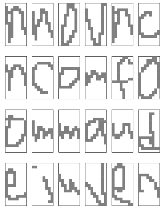
Figure 2: Eight example words from the handwriting recognition data set.

The handwriting recognition task we consider was introduced by kassel95handwriting. Later, taskar03mmmn presented state-of-the-art results on this task using max-margin Markov networks. The task is an image recognition task: the input is a sequence of pre-segmented hand-drawn letters and the output is the character sequence (“a”-“z”) in these images. The data set we consider is identical to that considered by taskar03mmmn and includes 6600 sequences (words) collected from 150 subjects. The average word contains $8$ characters. The images are $8\times 16$ pixels in size, and rasterized into a binary representation. Example image sequences are shown in Figure 2 (the first characters are removed because they are capitalized).

For each possible output letter, there is a unique feature that counts how many times that letter appears in the output. Furthermore, for each pair of letters, there is an “edge” feature counting how many times this pair appears adjacent in the output. These edge features are the only “structural features” used for this task (i.e., features that span multiple output labels). Finally, for every output letter and for every pixel position, there is a feature that counts how many times that pixel position is “on” for the given output letter.

In the experiments, we consider two variants of the data set. The first, “small,” is the problem considered by taskar03mmmn. In the small problem, ten fold cross-validation is performed over the data set; in each fold, roughly 600 words are used as training data and the remaining 6000 are used as test data. In addition to this setting, we also consider the “large” reverse experiment: in each fold, 6000 words are used as training data and 600 are used as test data.

6.1.2 Spanish Named Entity Recognition

El presidente de la [Junta de Extremadura]${}_{\textsf{ORG}}$ , [Juan Carlos Rodríguez Ibarra]${}_{\textsf{PER}}$ , recibirá en la sede de la [Presidencia del Gobierno]${}_{\textsf{ORG}}$ extremeño a familiares de varios de los condenados por el proceso “ [Lasa-Zabala]${}_{\textsf{MISC}}$ ” , entre ellos a [Lourdes Díez Urraca]${}_{\textsf{PER}}$ , esposa del ex gobernador civil de [Guipúzcoa]${}_{\textsf{LOC}}$ [Julen Elgorriaga]${}_{\textsf{PER}}$ ; y a [Antonio Rodríguez Galindo]${}_{\textsf{PER}}$ , hermano del general [Enrique Rodríguez Galindo]${}_{\textsf{PER}}$ .

Figure 3: Example labeled sentence from the Spanish Named Entity Recognition task.

The named entity recognition (NER) task is concerned with spotting names of persons, places and organizations in text. Moreover, in NER we only aim to spot names and neither pronouns (“he”) nor nominal references (“the President”). We use the CoNLL 2002 data set, which consists of $8324$ training sentences and $1517$ test sentences; examples are shown in Figure 3. A $300$-sentence subset of the training data set was previously used by tsochantaridis05svmiso for evaluating the SVM${}^{\textnormal{struct}}$ framework in the context of sequence labeling. The small training set was likely used for computational considerations. The best reported results to date using the full data set are due to ando05transfer. We report results on both the “small” and “large” data sets.

The structural features used for this task are roughly the same as in the handwriting recognition case. For each label, each label pair and each label triple, a feature counts the number of times this element is observed in the output. Furthermore, the standard set of input features includes the words and simple functions of the words (case markings, prefix and suffix up to three characters) within a window of $\pm 2$ around the current position. These input features are paired with the current label. This feature set is fairly standard in the literature, though ando05transfer report significantly improved results using a much larger set of features. In the results shown later in this section, all comparison algorithms use identical feature sets.

6.1.3 Syntactic Chunking

[Great American]${}_{\textsf{NP}}$ [said]${}_{\textsf{VP}}$ [it]${}_{\textsf{NP}}$ [increased]${}_{\textsf{VP}}$ [its loan-loss reserves]${}_{\textsf{NP}}$ [by]${}_{\textsf{PP}}$ [$ 93 million]${}_{\textsf{NP}}$ [after]${}_{\textsf{PP}}$ [reviewing]${}_{\textsf{VP}}$ [its loan portfolio]${}_{\textsf{NP}}$ , [raising]${}_{\textsf{VP}}$ [its total loan and real estate reserves]${}_{\textsf{NP}}$ [to]${}_{\textsf{PP}}$ [$ 217 million]${}_{\textsf{NP}}$ .

Figure 4: Example labeled sentence from the syntactic chunking task.