A Bayesian Model for Discovering Typological Implications

Abstract

A standard form of analysis for linguistic typology is the universal implication. These implications state facts about the range of extant languages, such as “if objects come after verbs, then adjectives come after nouns.” Such implications are typically discovered by painstaking hand analysis over a small sample of languages. We propose a computational model for assisting at this process. Our model is able to discover both well-known implications as well as some novel implications that deserve further study. Moreover, through a careful application of hierarchical analysis, we are able to cope with the well-known sampling problem: languages are not independent.

1 Introduction

Linguistic typology aims to distinguish between logically possible languages and actually observed languages. A fundamental building block for such an understanding is the universal implication [Greenberg, 1963]. These are short statements that restrict the space of languages in a concrete way (for instance “object-verb ordering implies adjective-noun ordering”); ?), ?) and ?) provide excellent introductions to linguistic typology. We present a statistical model for automatically discovering such implications from a large typological database [Haspelmath et al., 2005].

Analyses of universal implications are typically performed by linguists, inspecting an array of $30$-$100$ languages and a few pairs of features. Looking at all pairs of features (typically several hundred) is virtually impossible by hand. Moreover, it is insufficient to simply look at counts. For instance, results presented in the form “verb precedes object implies prepositions in 16/19 languages” are nonconclusive. While compelling, this is not enough evidence to decide if this is a statistically well-founded implication. For one, maybe $99\%$ of languages have prepositions: then the fact that we’ve achieved a rate of $84\%$ actually seems really bad. Moreover, if the $16$ languages are highly related historically or areally (geographically), and the other $3$ are not, then we may have only learned something about geography.

In this work, we propose a statistical model that deals cleanly with these difficulties. By building a computational model, it is possible to apply it to a very large typological database and search over many thousands of pairs of features. Our model hinges on two novel components: a statistical noise model a hierarchical inference over language families. To our knowledge, there is no prior work directly in this area. The closest work is represented by the books Possible and Probable Languages [Newmeyer, 2005] and Language Classification by Numbers [McMahon and McMahon, 2005], but the focus of these books is on automatically discovering phylogenetic trees for languages based on Indo-European cognate sets [Dyen et al., 1992].

2 Data

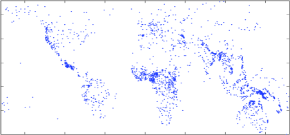
Figure 1: Map of the $2150$ languages in the database.

	Numeral			Glottalized		Number of
Language	Classifiers	Rel/N Order	O/V Order	Consonants	Tone	Genders
English	Absent	NRel	VO	None	None	Three
Hindi	Absent	RelN	OV	None	None	Two
Mandarin	Obligatory	RelN	VO	None	Complex	None
Russian	Absent	NRel	VO	None	None	Three
Tukang Besi	Absent	?	Either	Implosives	None	Three
Zulu	Absent	NRel	VO	Ejectives	Simple	Five+

Table 1: Example database entries for a selection of diverse languages and features.

The database on which we perform our analysis is the World Atlas of Language Structures [Haspelmath et al., 2005]. This database contains information about $2150$ languages (sampled from across the world; Figure 1 depicts the locations of languages). There are $139$ features in this database, broken down into categories such as “Nominal Categories,” “Simple Clauses,” “Phonology,” “Word Order,” etc. The database is sparse: for many language/feature pairs, the feature value is unknown. In fact, only about $16\%$ of all possible language/feature pairs are known. A sample of five languages and six features from the database are shown in Table 1.

Importantly, the density of samples is not random. For certain languages (eg., English, Chinese, Russian), nearly all features are known, whereas other languages (eg., Asturian, Omagua, Frisian) that have fewer than five feature values known. Furthermore, some features are known for many languages. This is due to the fact that certain features take less effort to identify than others. Identifying, for instance, if a language has a particular set of phonological features (such as glottalized consonants) requires only listening to speakers. Other features, such as determining the order of relative clauses and nouns require understanding much more of the language.

3 Models

In this section, we propose two models for automatically uncovering universal implications from noisy, sparse data. First, note that even well attested implications are not always exceptionless. A common example is that verbs preceding objects (“VO”) implies adjectives following nouns (“NA”). This implication (VO $\supset$ NA) has one glaring exception: English. This is one particular form of noise. Another source of noise stems from transcription. WALS contains data about languages documented by field linguists as early as the 1900s. Much of this older data was collected before there was significant agreement in documentation style. Different field linguists often had different dimensions along which they segmented language features into classes. This leads to noise in the properties of individual languages.

Another difficulty stems from the sampling problem. This is a well-documented issue (see, eg., [Croft, 2003]) stemming from the fact that any set of languages is not sampled uniformly from the space of all probable languages. Politically interesting languages (eg., Indo-European) and typologically unusual languages (eg., Dyirbal) are better documented than others. Moreover, languages are not independent: German and Dutch are more similar than German and Hindi due to history and geography.

The first model, Flat, treats each language as independent. It is thus susceptible to sampling problems. For instance, the WALS database contains a half dozen versions of German. The Flat model considers these versions of German just as statistically independent as, say, German and Hindi. To cope with this problem, we then augment the Flat model into a Hierarchical model that takes advantage of known hierarchies in linguistic phylogenetics. The Hier model explicitly models the fact that individual languages are not independent and exhibit strong familial dependencies. In both models, we initially restrict our attention to pairs of features. We will describe our models as if all features are binary. We expand any multi-valued feature with $K$ values into $K$ binary features in a “one versus rest” manner.

3.1 The Flat Model

In the Flat model, we consider a $2\times N$ matrix of feature values. The $N$ corresponds to the number of languages, while the $2$ corresponds to the two features currently under consideration (eg., object/verb order and noun/adjective order). The order of the two features is important: $f_{1}$ implies $f_{2}$ is logically different from $f_{2}$ implies $f_{1}$. Some of the entries in the matrix will be unknown. We may safely remove all languages from consideration for which both are unknown, but we do not remove languages for which only one is unknown. We do so because our model needs to capture the fact that if $f_{2}$ is always true, then $f_{1}\supset f_{2}$ is uninteresting.

The statistical model is set up as follows. There is a single variable (we will denote this variable “$m$”) corresponding to whether the implication holds. Thus, $m=1$ means that $f_{1}$ implies $f_{2}$ and $m=0$ means that it does not. Independent of $m$, we specify two feature priors, $\pi_{1}$ and $\pi_{2}$ for $f_{1}$ and $f_{2}$ respectively. $\pi_{1}$ specifies the prior probability that $f_{1}$ will be true, and $\pi_{2}$ specifies the prior probability that $f_{2}$ will be true. One can then put the model together naïvely as follows. If $m=0$ (i.e., the implication does not hold), then the entire data matrix is generated by choosing values for $f_{1}$ (resp., $f_{2}$) independently according to the prior probability $\pi_{1}$ (resp., $\pi_{2}$). On the other hand, if $m=1$ (i.e., the implication does hold), then the first column of the data matrix is generated by choosing values for $f_{1}$ independently by $\pi_{1}$, but the second column is generated differently. In particular, if for a particular language, we have that $f_{1}$ is true, then the fact that the implication holds means that $f_{2}$ must be true. On the other hand, if $f_{1}$ is false for a particular language, then we may generate $f_{2}$ according to the prior probability $\pi_{2}$. Thus, having $m=1$ means that the model is significantly more constrained. In equations:

$$p(f_{1}\textrm{~{}}\arrowvert\textrm{~{}}\pi_{1}) =\pi_{1}^{f_{1}}(1-\pi_{1})^{1-f_{1}}$$

$$p(f_{2}\textrm{~{}}\arrowvert\textrm{~{}}f_{1},\pi_{2},m) =\left\{\begin{array}[]{ll}f_{2}&m=f_{1}=1\\ \pi_{2}^{f_{2}}(1-\pi_{2})^{1-f_{2}}&\text{otherwise}\end{array}\right.$$

The problem with this naïve model is that it does not take into account the fact that there is “noise” in the data. (By noise, we refer either to mis-annotations, or to “strange” languages like English.) To account for this, we introduce a simple noise model. There are several options for parameterizing the noise, depending on what independence assumptions we wish to make. One could simply specify a noise rate for the entire data set. One could alternatively specify a language-specific noise rate. Or one could specify a feature-specific noise rate. We opt for a blend between the first and second option. We assume an underlying noise rate for the entire data set, but that, conditioned on this underlying rate, there is a language-specific noise level. We believe this to be an appropriate noise model because it models the fact that the majority of information for a single language is from a single source. Thus, if there is an error in the database, it is more likely that other errors will be for the same languages.

In order to model this statistically, we assume that there are latent variables $e_{1,n}$ and $e_{2,n}$ for each language $n$. If $e_{1,n}=1$, then the first feature for language $n$ is wrong. Similarly, if $e_{2,n}=1$, then the second feature for language $n$ is wrong. Given this model, the probabilities are exactly as in the naïve model, with the exception that instead of using $f_{1}$ (resp., $f_{2}$), we use the exclusive-or $f_{1}\otimes e_{1}$ (resp., $f_{2}\otimes e_{2}$) so that the feature values are flipped whenever the noise model suggests an error.

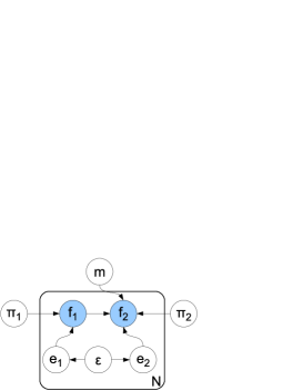
Figure 2: Graphical model for the Flat model.

The graphical model for the Flat model is shown in Figure 2. Circular nodes denote random variables and arrows denote conditional dependencies. The rectangular plate denotes the fact that the elements contained within it are replicated $N$ times ($N$ is the number of languages). In this model, there are four “root” nodes: the implication value $m$; the two feature prior probabilities $\pi_{1}$ and $\pi_{2}$; and the language-specific error rate $\epsilon$. On all of these nodes we place Bayesian priors. Since $m$ is a binary random variable, we place a Bernoulli prior on it. The $\pi$s are Bernoulli random variables, so they are given independent Beta priors. Finally, the noise rate $\epsilon$ is also given a Beta prior. For the two Beta parameters governing the error rate (i.e., $a_{\epsilon}$ and $b_{\epsilon}$) we set these by hand so that the mean expected error rate is $5\%$ and the probability of the error rate being between $0\%$ and $10\%$ is $50\%$ (this number is based on an expert opinion of the noise-rate in the data). For the rest of the parameters we use uniform priors.

3.2 The Hier Model

A significant difficulty in working with any large typological database is that the languages will be sampled nonuniformly. In our case, this means that implications that seem true in the Flat model may only be true for, say, Indo-European, and the remaining languages are considered noise. While this may be interesting in its own right, we are more interested in discovering implications that are truly universal.

We model this using a hierarchical Bayesian model. In essence, we take the Flat model and build a notion of language relatedness into it. In particular, we enforce a hierarchy on the $m$ implication variables. For simplicity, suppose that our “hierarchy” of languages is nearly flat. Of the $N$ languages, half of them are Indo-European and the other half are Austronesian. We will use a nearly identical model to the Flat model, but instead of having a single $m$ variable, we have three: one for IE, one for Austronesian and one for “all languages.”

For a general tree, we assign one implication variable for each node (including the root and leaves). The goal of the inference is to infer the value of the $m$ variable corresponding to the root of the tree.

All that is left to specify the full Hier model is to specify the probability distribution of the $m$ random variables. We do this as follows. We place a zero mean Gaussian prior with (unknown) variance $\sigma^{2}$ on the root $m$. Then, for a non-root node, we use a Gaussian with mean equal to the “$m$” value of the parent and tied variance $\sigma^{2}$. In our three-node example, this means that the root is distributed $\mathcal{N}\textit{or}(0,\sigma^{2})$ and each child is distributed $\mathcal{N}\textit{or}(m_{\text{root}},\sigma^{2})$, where $m_{\text{root}}$ is the random variable corresponding to the root. Finally, the leaves (corresponding to the languages themselves) are distributed logistic-binomial. Thus, the $m$ random variable corresponding to a leaf (language) is distributed $\mathcal{B}\textit{in}(s(m_{\text{par}}))$, where $m_{\text{par}}$ is the $m$ value for the parent (internal) node and $s$ is the sigmoid function $s(x)=[1+exp(-x)]^{-1}$.

The intuition behind this model is that the $m$ value at each node in the tree (where a node is either “all languages” or a specific language family or an individual language) specifies the extent to which the implication under consideration holds for that node. A large positive $m$ means that the implication is very likely to hold. A large negative value means it is very likely to not hold. The normal distributions across edges in the tree indicate that we expect the $m$ values not to change too much across the tree. At the leaves (i.e., individual languages), the logistic-binomial simply transforms the real-valued $m$s into the range $[0,1]$ so as to make an appropriate input to the binomial distribution.

4 Statistical Inference

In this section, we describe how we use Markov chain Monte Carlo methods to perform inference in the statistical models described in the previous section; ?) provide an excellent introduction to MCMC techniques. The key idea behind MCMC techniques is to approximate intractable expectations by drawing random samples from the probability distribution of interest. The expectation can then be approximated by an empirical expectation over these sample.

For the Flat model, we use a combination of Gibbs sampling with rejection sampling as a subroutine. Essentially, all sampling steps are standard Gibbs steps, except for sampling the error rates $e$. The Gibbs step is not available analytically for these. Hence, we use rejection sampling (drawing from the Beta prior and accepting according to the posterior).

The sampling procedure for the Hier model is only slightly more complicated. Instead of performing a simple Gibbs sample for $m$ in Step (4), we first sample the $m$ values for the internal nodes using simple Gibbs updates. For the leaf nodes, we use rejection sampling. For this rejection, we draw proposal values from the Gaussian specified by the parent $m$, and compute acceptance probabilities.

In all cases, we run the outer Gibbs sampler for $1000$ iterations and each rejection sampler for $20$ iterations. We compute the marginal values for the $m$ implication variables by averaging the sampled values after dropping $200$ “burn-in” iterations.

5 Data Preprocessing and Search

After extracting the raw data from the WALS electronic database [Haspelmath et al., 2005], we perform a minor amount of preprocessing. Essentially, we have manually removed certain feature values from the database because they are underrepresented. For instance, the “Glottalized Consonants” feature has eight possible values (one for “none” and seven for different varieties of glottalized consonants). We reduce this to simply two values “has” or “has not.” $313$ languages have no glottalized consonants and $139$ have some variety of glottalized consonant. We have done something similar with approximately twenty of the features.

For the Hier model, we obtain the hierarchy in one of two ways. The first hierarchy we use is the “linguistic hierarchy” specified as part of the WALS data. This hierarchy divides languages into families and subfamilies. This leads to a tree with the leaves at depth four. The root has $38$ immediate children (corresponding to the major families), and there are a total of $314$ internal nodes. The second hierarchy we use is an areal hierarchy obtained by clustering languages according to their latitude and longitude. For the clustering we first cluster all the languages into $6$ “macro-clusters.” We then cluster each macro-cluster individually into $25$ “micro-clusters.” These micro-clusters then have the languages at their leaves. This yields a tree with $31$ internal nodes.

Given the database (which contains approximately $140$ features), performing a raw search even over all possible pairs of features would lead to over $19,000$ computations. In order to reduce this space to a more manageable number, we filter:

• There must be at least $250$ languages for which both features are known.

• There must be at least $15$ languages for which both feature values hold simultaneously.

• Whenever $f_{1}$ is true, at least half of the languages also have $f_{2}$ true.

Performing all these filtration steps reduces the number of pairs under consideration to $3442$. While this remains a computationally expensive procedure, we were able to perform all the implication computations for these $3442$ possible pairs in about a week on a single modern machine (in Matlab).

6 Results

The task of discovering universal implications is, at its heart, a data-mining task. As such, it is difficult to evaluate, since we often do not know the correct answers! If our model only found well-documented implications, this would be interesting but useless from the perspective of aiding linguists focus their energies on new, plausible implications. In this section, we present the results of our method, together with both a quantitative and qualitative evaluation.

6.1 Quantitative Evaluation

In this section, we perform a quantitative evaluation of the results based on predictive power. That is, one generally would prefer a system that finds implications that hold with high probability across the data. The word “generally” is important: this quality is neither necessary nor sufficient for the model to be good. For instance, finding $1000$ implications of the form $A_{1}\supset X,A_{2}\supset X,\dots,A_{1000}\supset X$ is completely uninteresting if $X$ is true in $99\%$ of the cases. Similarly, suppose that a model can find $1000$ implications of the form $X\supset A_{1},\dots,X\supset A_{1000}$, but $X$ is only true in five languages. In both of these cases, according to a “predictive power” measure, these would be ideal systems. But they are both somewhat uninteresting.

Despite these difficulties with a predictive power-based evaluation, we feel that it is a good way to understand the relative merits of our different models. Thus, we compare the following systems: Flat (our proposed flat model), LingHier (our model using the phylogenetic hierarchy), DistHier (our model using the areal hierarchy) and Random (a model that ranks implications—that meet the three qualifications from the previous section—randomly).

The models are scored as follows. We take the entire WALS data set and “hide” a random $10\%$ of the entries. We then perform full inference and ask the inferred model to predict the missing values. The accuracy of the model is the accuracy of its predictions. To obtain a sense of the quality of the ranking, we perform this computation on the top $k$ ranked implications provided by each model; $k\in\{2,4,8,\dots,512,1024\}$.

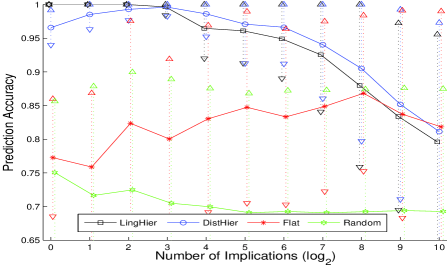
Figure 3: Results of quantitative (predictive) evaluation. Top curves are the hierarchical models; middle is the flat model; bottom is the random baseline.

The results of this quantitative evaluation are shown in Figure 3 (on a log-scale for the x-axis). The two best-performing models are the two hierarchical models. The flat model does significantly worse and the random model does terribly. The vertical lines are a standard deviation over $100$ folds of the experiment (hiding a different $10\%$ each time). The difference between the two hierarchical models is typically not statistically significant. At the top of the ranking, the model based on phylogenetic information performs marginally better; at the bottom of the ranking, the order flips. Comparing the hierarchical models to the flat model, we see that adequately modeling the a priori similarity between languages is quite important.

6.2 Cross-model Comparison

The results in the previous section support the conclusion that the two hierarchical models are doing something significantly different (and better) than the flat model. This clearly must be the case. The results, however, do not say whether the two hierarchies are substantially different. Moreover, are the results that they produce substantially different. The answer to these two questions is “yes.”

We first address the issue of tree similarity. We consider all pairs of languages which are at distance $0$ in the areal tree (i.e., have the same parent). We then look at the mean tree-distance between those languages in the phylogenetic tree. We do this for all distances in the areal tree (because of its construction, there are only three: $0$, $2$ and $4$). The mean distances in the phylogenetic tree corresponding to these three distances in the areal tree are: $2.9$, $3.5$ and $4.0$, respectively. This means that languages that are “nearby” in the areal tree are quite often very far apart in the phylogenetic tree.

To answer the issue of whether the results obtained by the two trees are similar, we employ Kendall’s $\tau$ statistic. Given two ordered lists, the $\tau$ statistic computes how correlated they are. $\tau$ is always between $0$ and $1$, with $1$ indicating identical ordering and $0$ indicated completely reversed ordering. The results are as follows. Comparing Flat to LingHier yield $\tau=0.4144$, a very low correlation. Between Flat and DistHier, $\tau=0.5213$, also very low. These two are as expected. Finally, between LingHier and DistHier, we obtain $\tau=0.5369$, a very low correlation, considering that both perform well predictively.

6.3 Qualitative Analysis

For the purpose of a qualitative analysis, we reproduce the top $30$ implications discovered by the LingHier model in Table 2 (see the final page). Each implication is numbered, then the actual implication is presented. For instance, #7 says that any language that has adjectives preceding their governing nouns also has numerals preceding their nouns. We additionally provide an “analysis” of many of these discovered implications. Many of them (eg., #7) are well known in the typological literature. These are simply numbered according to well-known references. For instance our #7 is implication #18 from Greenberg, reproduced by ?). Those that reference Hawkins (eg., #11) are based on implications described by ?); those that reference Lehmann are references to the principles decided by ?) in Ch 4 & 8.

Some of the implications our model discovers are obtained by composition of well-known implications. For instance, our #3 (namely, OV $\supset$ Genitive-Noun) can be obtained by combining Greenberg #4 (OV $\supset$ Postpositions) and Greenberg #2a (Postpositions $\supset$ Genitive-Noun). It is quite encouraging that $14$ of our top $21$ discovered implications are well-known in the literature (and this, not even considering the tautalogically true implications)! This strongly suggests that our model is doing something reasonable and that there is true structure in the data.

In addition to many of the known implications found by our model, there are many that are “unknown.” Space precludes attempting explanations of them all, so we focus on a few. Some are easy. Consider #8 (Strongly suffixing $\supset$ Tense-aspect suffixes): this is quite plausible—if you have a language that tends to have suffixes, it will probably have suffixes for tense/aspect. Similarly, #10 states that languages with verb morphology for questions lack question particles; again, this can be easily explained by an appeal to economy.

Some of the discovered implications require a more involved explanation. One such example is #20: labial-velars implies no uvulars. It turns out that labial-velars are most common in Africa just north of the equator, which is also a place that has very few uvulars (there are a handful of other examples, mostly in Papua New Guinea). While this implication has not been previously investigated, it makes some sense: if a language has one form of rare consonant, it is unlikely to have another.

As another example, consider #28: Obligatory suffix pronouns implies no possessive affixes. This means is that in languages (like English) for which pro-drop is impossible, possession is not marked morphologically on the head noun (like English, “book” appears the same regarless of if it is “his book” or “the book”). This also makes sense: if you cannot drop pronouns, then one usually will mark possession on the pronoun, not the head noun. Thus, you do not need marking on the head noun.

Finally, consider #25: High and mid front vowels (i.e., / u/, etc.) implies large vowel inventory ($\geq 7$ vowels). This is supported by typological evidence that high and mid front vowels are the “last” vowels to be added to a language’s repertoire. Thus, in order to get them, you must also have many other types of vowels already, leading to a large vowel inventory.

Not all examples admit a simple explanation and are worthy of further thought. Some of which (like the ones predicated on “SV”) may just be peculiarities of the annotation style: the subject verb order changes frequently between transitive and intransitive usages in many languages, and the annotation reflects just one. Some others are bizzarre: why not having fricatives should mean that you don’t have tones (#27) is not a priori clear.

#	Implicant $\supset$	Implicand	Analysis
1	Postpositions $\supset$	Genitive-Noun	Greenberg #2a
2	OV $\supset$	Postpositions	Greenberg #4
3	OV $\supset$	Genitive-Noun	Greenberg #4 + Greenberg #2a
4	Genitive-Noun $\supset$	Postpositions	Greenberg #2a (converse)
5	Postpositions $\supset$	OV	Greenberg #2b (converse)
6	SV $\supset$	Genitive-Noun	???
7	Adjective-Noun $\supset$	Numeral-Noun	Greenberg #18
8	Strongly suffixing $\supset$	Tense-aspect suffixes	Clear explanation
9	VO $\supset$	Noun-Relative Clause	Lehmann
10	Interrogative verb morph $\supset$	No question particle	Appeal to economy
11	Numeral-Noun $\supset$	Demonstrative-Noun	Hawkins XVI (for postpositional languages)
12	Prepositions $\supset$	VO	Greenberg #3 (converse)
13	Adjective-Noun $\supset$	Demonstrative-Noun	Greenberg #18
14	Noun-Adjective $\supset$	Postpositions	Lehmann
15	SV $\supset$	Postpositions	???
16	VO $\supset$	Prepositions	Greenberg #3
17	Initial subordinator word $\supset$	Prepositions	Operator-operand principle (Lehmann)
18	Strong prefixing $\supset$	Prepositions	Greenberg #27b
19	Little affixation $\supset$	Noun-Adjective	???
20	Labial-velars $\supset$	No uvular consonants	See text
21	Negative word $\supset$	No pronominal possessive affixes	See text
22	Strong prefixing $\supset$	VO	Lehmann
23	Subordinating suffix $\supset$	Strongly suffixing	???
24	Final subordinator word $\supset$	Postpositions	Operator-operand principle (Lehmann)
25	High and mid front vowels $\supset$	Large vowel inventories	See text
26	Plural prefix $\supset$	Noun-Genitive	???
27	No fricatives $\supset$	No tones	???
28	Obligatory subject pronouns $\supset$	No pronominal possessive affixes	See text
29	Demonstrative-Noun $\supset$	Tense-aspect suffixes	Operator-operand principle (Lehmann)
30	Prepositions $\supset$	Noun-Relative clause	Lehmann, Hawkins

Table 2: Top $30$ implications discovered by the LingHier model.

6.4 Multi-conditional Implications

Many implications in the literature have multiple implicants. For instance, much research has gone into looking at which implications hold, considering only “VO” languages, or considering only languages with prepositions. It is straightforward to modify our model so that it searches over triples of features, conditioning on two and predicting the third. Space precludes an in-depth discussion of these results, but we present the top examples in Table 3 (after removing the tautalogically true examples, which are more numerous in this case, as well as examples that are directly obtainable from Table 2). It is encouraging that in the top $1000$ multi-conditional implications found, the most frequently used were “OV” ($176$ times) “Postpositions” ($157$ times) and “Adjective-Noun” ($89$ times). This result agrees with intuition.

Implicants		Implicand
Postpositions	$\supset$	Demonstrative-Noun
Adjective-Noun
Posessive prefixes	$\supset$	Genitive-Noun
Tense-aspect suffixes
Case suffixes	$\supset$	Genitive-Noun
Plural suffix
Adjective-Noun	$\supset$	OV
Genitive-Noun
High cons/vowel ratio	$\supset$	No tones
No front-rounded vowels
Negative affix	$\supset$	OV
Genitive-Noun
No front-rounded vowels	$\supset$	Large vowel quality inventory
Labial velars
Subordinating suffix	$\supset$	Postpositions
Tense-aspect suffixes
No case affixes	$\supset$	Initial subordinator word
Prepositions
Strongly suffixing	$\supset$	Genitive-Noun
Plural suffix

Table 3: Top implications discovered by the LingHier multi-conditional model.

7 Discussion

We have presented a Bayesian model for discovering universal linguistic implications from a typological database. Our model is able to account for noise in a linguistically plausible manner. Our hierarchical models deal with the sampling issue in a unique way, by using prior knowledge about language families to “group” related languages. Quantitatively, the hierarchical information turns out to be quite useful, regardless of whether it is phylogenetically- or areally-based. Qualitatively, our model can recover many well-known implications as well as many more potential implications that can be the object of future linguistic study. We believe that our model is sufficiently general that it could be applied to many different typological databases — we attempted not to “overfit” it to WALS. Our hope is that the automatic discovery of such implications not only aid typologically-inclined linguists, but also other groups. For instance, well-attested universal implications have the potential to reduce the amount of data field linguists need to collect. They have also been used computationally to aid in the learning of unsupervised part of speech taggers [Schone and Jurafsky, 2001]. Many extensions are possible to this model; for instance attempting to uncover typologically hierarchies and other higher-order structures. We have made the full output of all models available at http://hal3.name/WALS.

Acknowledgments.

We are grateful to Yee Whye Teh, Eric Xing and three anonymous reviewers for their feedback on this work.

References

- [1]
- [Andrieu et al., 2003] Christophe Andrieu, Nando de Freitas, Arnaud Doucet, and Michael I. Jordan. 2003. An introduction to MCMC for machine learning. Machine Learning (ML), 50:5–43.
- [Croft, 2003] William Croft. 2003. Typology and Univerals. Cambridge University Press.
- [Dyen et al., 1992] Isidore Dyen, Joseph Kurskal, and Paul Black. 1992. An Indoeuropean classification: A lexicostatistical experiment. Transactions of the American Philosophical Society, 82(5). American Philosophical Society.
- [Greenberg, 1963] Joseph Greenberg, editor. 1963. Universals of Languages. MIT Press.
- [Haspelmath et al., 2005] Martin Haspelmath, Matthew Dryer, David Gil, and Bernard Comrie, editors. 2005. The World Atlas of Language Structures. Oxford University Press.
- [Hawkins, 1983] John A. Hawkins. 1983. Word Order Universals: Quantitative analyses of linguistic structure. Academic Press.
- [Lehmann, 1981] Winfred Lehmann, editor. 1981. Syntactic Typology, volume xiv. University of Texas Press.
- [McMahon and McMahon, 2005] April McMahon and Robert McMahon. 2005. Language Classification by Numbers. Oxford University Press.
- [Newmeyer, 2005] Frederick J. Newmeyer. 2005. Possible and Probable Languages: A Generative Perspective on Linguistic Typology. Oxford University Press.
- [Schone and Jurafsky, 2001] Patrick Schone and Dan Jurafsky. 2001 Language Independent Induction of Part of Speech Class Labels Using only Language Universals. Machine Learning: Beyond Supervision.
- [Song, 2001] Jae Jung Song. 2001. Linguistic Typology: Morphology and Syntax. Longman Linguistics Library.