On resonance parameter measurement and luminosity determination at $e^{+}e^{-}$ collider

1 Introduction

Resonance are a special kind of particles and their study is of great interest and importance in the domain of elementary particle physics. Measurements of resonance parameters, such as the mass ($M_{R}$), total decay width ($\Gamma_{t}$), partial decay width of final state $f$ ($\Gamma_{f}$, where $f=e,\mu,\tau$ indicating the $e$-pair, $\mu$-pair, and $\tau$-pair final states, respectively), and corresponding branching ratios are fundamental work for high energy experimental physics. For resonances of $1^{--}$ charmonium and bottomnium, such as $J/\psi$, $\psi^{\prime}$, $\psi^{\prime\prime}$, $\cdots$, $\Upsilon(nS),(n=1,2,3,4,\cdots)$ $etc$, their resonance parameters can be measured by scan experiment at $e^{+}e^{-}$ colliders [1]-[13], which is one of basic approaches to understand resonances in collision experiment.

For the experiment using scan method, data are taken at several different energy points in the vicinity of the resonance to be measured. The minimization technique is usually applied on the estimator which constructed by the difference between the measured number of events and the expected number of events. The latter can be obtained by theoretical calculation and Monte carlo simulation. Specially, the expected number of events for certain final state $f$ at the point with center-of-mass energy $W$ can be obtained by the expression

$$N_{f}(W,\vec{\eta})=L(W)\cdot\sigma^{obs}_{f}(W,\vec{\eta})~{},$$ (1)

where $\vec{\eta}$ is the parameter vector which contains the information of resonance parameters. $\sigma^{obs}$ is the experimentally observed cross section (the detailed description refer to section 3) which is the synthetic cross section including resonance part, continuum part, and their interference; and also incorporating the effect due to experiment efficiency. $L$ is the luminosity which can be acquired through several approaches.

Figure 1: Differential cross sections for three QED processes: $e^{+}e^{-}\to e^{+}e^{-}$, $e^{+}e^{-}\to\mu^{+}\mu^{-}$, and $e^{+}e^{-}\to\gamma\gamma$. The center-of-mass energy is 3.5 GeV.

In principle any detectable process can be used for luminosity measurement. However in order to achieve high precision, one often selects the process which has larger cross section and salient characteristic topology experimentally with accurate theoretical calculation of the cross section. From these point of view, the QED processes such as $e^{+}e^{-}\to e^{+}e^{-}$, $e^{+}e^{-}\to\mu^{+}\mu^{-}$, and $e^{+}e^{-}\to\gamma\gamma$, are most often adopted for luminosity measurements [14]. The lowest order of differential cross sections for these processes are shown in Fig. 1. Experimentally, the response of the detector to each of these reactions is quite distinct: efficiencies rely on the charged particle tracking ($e^{+}e^{-}$), calorimetry ($e^{+}e^{-}$ and $\gamma\gamma$), muon counter ($\mu^{+}\mu^{-}$), and trigger algorithms. The expected theoretical cross sections are calculable in quantum electrodynamics; weak interaction effects are negligible for charm and B-factories at the level of 1 per mill. [15].

For luminosity measurement, the interference effect in the vicinity of resonance peaks has to be treated with great care. Such effect not only distorts the cross section in the peak region but also shifts the resonance peak position. Especially, when the cross sections of resonance and non-resonance processes are compatible, the interference effect are too prominent to be neglected. In such circumstance, when we consider how to determine the luminosity, we come across a dilemma. On one hand, to determine the luminosity we must subtract the contributions due to resonances and corresponding interference effect. This can be realized by correct determination of resonance parameters. On the other hand, the measurement of resonance parameters depends on the accurate determination of luminosity. That is to say the measurement of resonance parameter and determination of luminosity are the cause-consequence interdependence. To resolve such an intertwist issue, we recourse to an iteration approach which will be expounded in section 4. Before that, in section 2 and 3, presented are the formulas for experimentally observed cross section which take into account various experimental effects at $e^{+}e^{-}$ collider such as vacuum polarization, initial radiative correction, and beam energy spread.

2 Cross Section for $1^{--}$ resonance

In this section, we discuss in detail the experimental corrections on cross section and provide the analytic expressions for calculation of experimentally observed cross section.

2.1 Experimental corrections

The cross section of the resonance process

$$e^{+}e^{-}\rightarrow\mbox{Res.}\rightarrow f~{},$$ (2)

where $f$ denotes a certain kind of final state, is described by the Breit-Wigner formula

$$\sigma_{BW}(W)=\frac{12\pi\cdot\Gamma_{e}\Gamma_{f}}{(W^{2}-M^{2})^{2}+\Gamma^{2}M^{2}},$$ (3)

where $W$ is the center-of-mass energy, $\Gamma_{e}$ and $\Gamma_{f}$ are the widths of the resonance decaying into $e^{+}e^{-}$ and $f$, $\Gamma$ and $M$ are the total width and mass of resonance. Taking the initial state radiative (ISR) correction into consideration, the cross section becomes [16]

$$\sigma_{r.c.}(W)=\int\limits_{0}^{x_{m}}dxF(x,s)\frac{1}{|1-\Pi(s(1-x))|^{2}}\sigma_{BW}(s(1-x)),$$ (4)

where $s=W^{2}$, $x_{m}=1-s^{\prime}/s$, $\sqrt{s^{\prime}}$ is the experimentally required minimum invariant mass of the final state $f$ after losing energy due to multi-photon emission; $F(x,s)$ has been calculated in many references [16, 17, 18, 19] and $\Pi(s(1-x))$ is the vacuum polarization factor. The radiative correction in the final states are usually not considered [20, 21]. The reasons are twofold. In the first place, the hadronic final system is very complicated and since the radiative corrections depend upon the details of how the experiment is done, it is difficult to give a general, model-independent prescription for them. The second reason is that our understanding of the hadronic problem is so crude that there is no need to worry about the electromagnetic corrections.

The $e^{+}e^{-}$ colliders have finite beam energy spread. The beam energy spread function $G(W,W^{\prime})$ is usually a Gaussian distribution:

$$G(W,W^{\prime})=\frac{1}{\sqrt{2\pi}\Delta}e^{-\frac{(W-W^{\prime})^{2}}{2{\Delta}^{2}}},$$ (5)

where $\Delta$ is the standard deviation of the Gaussian distribution. It varies with the beam energy of the collider. For narrow resonances such as $J/\psi$ and $\psi^{\prime}$, $\Delta$ is usually much wider than the resonance intrinsic width. Therefore the beam-spreaded resonance cross section is the radiatively corrected Breit-Wigner cross section folded with the energy spread function:

$$\sigma_{G}(W)=\int\limits_{0}^{\infty}dW^{\prime}\sigma_{r.c.}(W^{\prime})G(W^{\prime},W),$$ (6)

where $\sigma_{r.c.}$ is defined by Eq. (4).

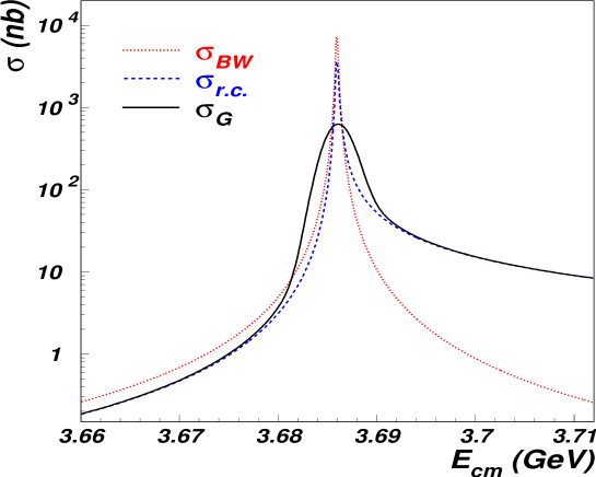
Figure 2: Inclusive hadronic cross sections for resonance of $\psi^{\prime}$: $\sigma_{BW}$ for Breit-Wigner cross section; $\sigma_{r.c.}$ the cross section with radiative correction; $\sigma_{G}$ the beam-spreaded cross section with the energy spread effect. In the calculation of these cross sections, the following parameters are used [13]: $M=3.68596$ GeV, $\Gamma_{t}=300$ keV, $\Gamma_{e}=2.19$ keV, and $\Delta=1.3$ MeV.

Take resonance $\psi^{\prime}$ as an example, Fig. 2 displays three cross sections: the Breit-Wigner cross section of Eq. (3); the cross section after radiative correction by Eq. (4), and the beam-spreaded cross section by Eq. (6). From the three curves in Fig. 2, it can be seen that the radiative correction reduces the height of the resonance. It also shifts the peak position to above the $\psi(2S)$ nominal mass. The reduction factor $\rho$ and the shift of the peak $\Delta\sqrt{s}_{max}$ are approximately expressed by [22]

$$\rho = {\displaystyle\left(\frac{\Gamma}{M}\right)^{t}\cdot(1+\delta)},$$ (7)

$$\Delta\sqrt{s}_{max} = {\displaystyle\frac{t\pi}{8}\Gamma},$$ (8)

where $t$ is defined as

$$t=\frac{2\alpha}{\pi}\left(\ln\frac{s}{m^{2}_{e}}-1\right),$$ (9)

with $\alpha$ and $m_{e}$ the QED fine structure constant and the mass of electron;

$$\delta=\frac{\alpha}{\pi}(\frac{\pi^{2}}{3}-\frac{1}{2})+\frac{3}{4}t+t^{2}(\frac{9}{32}-\frac{\pi^{2}}{12})$$ (10)

Herein the reduction factor $\rho$ is the ratio of the maximum resonance cross section with radiative correction to that of Born order.

At the $\psi^{\prime}$ mass, $t\approx 0.0779$ and $\delta\approx 0.06$, then the reduction factor $\rho\approx 0.51$ and the shift of the peak $\Delta\sqrt{s}_{max}\approx 9$ keV. The energy spread further lowers down and shifts the experimentally observed $\psi^{\prime}$ peak. In the case of a collider with $\Delta=1.3$ MeV, the maximum height of the $\psi(2S)$ peak becomes 640 nb, and the position of the peak is shifted by 0.14 MeV above the $\psi^{\prime}$ nominal mass.

From the example discussed above, the effects due to experimental corrections on resonance cross section are fairly prominent. For the continuum, effects are comparatively moderate [23]. Next, we will discuss in detail the ISR effect on Breit-Wigner cross section.

2.2 Initial state radiative correction

The ISR correction scheme used by earlier experiments, is based on the work of Bonneau and Martin [24] and that of Jackson and Scharre [25]. The former only calculated to $\alpha^{3}$ order which is insufficient for resonances; while the latter made some mistakes [26, 27]. The drawbacks due to the treatment of the radiative correction with these two schemes were studied for Z in Ref. [26] and for narrow resonances of $\psi$ and $\Upsilon$ families in Ref. [27]. In the eighties of the last century Kuraev and Fadin treats ISR correction based on the structure function approach which achieves 0.1% accuracy [16]. Afterwards such an approach is extensively used for ISR correction which is also followed in this paper.

The calculation of $F(x,s)$ is summarized in Ref [22]. But for the discussions on resonances in this paper, a different form derived in Ref [28] is more useful:

$$F(x,s)=x^{t-1}t\cdot(1+\delta)+x^{t}(-t-\frac{t^{2}}{4})+x^{t+1}(\frac{t}{2}-\frac{3}{8}t^{2})+{\cal O}(x^{t+2}t^{2})~{}.$$ (11)

Here the conversion of soft photons into real $e^{+}e^{-}$ pairs is included. Notice that $x<1$ and $t<1$, so the omitted terms in the above equation are small quantities. Then using equality [29]

$$\int\limits^{\infty}_{0}\frac{\nu x^{\nu-1}dx}{x^{2}+2ax\cos\beta+a^{2}}=a^{\nu-2}\cdot\frac{\pi\nu\sin[\beta(1-\nu)]}{\sin\beta\sin\pi\nu}~{}(\mbox{For }\nu<2)~{},$$ (12)

It can be obtained finally [28]

$$\sigma_{r.c.}(s)=\frac{12\pi\Gamma^{exp}_{e}\Gamma_{f}}{s^{2}}\cdot\left\{(1+\delta)t\cdot\frac{}{}\right.$$

$$\left[\frac{1}{t}\cdot a^{t-2}\phi(\cos\beta,t)+\frac{1}{t-2}+\frac{2(s-M^{2})}{(t-3)s}+\frac{3(s-M^{2})^{2}-M^{2}\Gamma^{2}}{(t-4)s^{2}}\right]$$

$$-t\left(1+\frac{t}{4}\right)\cdot$$

$$\left[\frac{1}{(t+1)}\cdot a^{t-1}\phi(\cos\beta,t+1)+\frac{1}{t-1}+\frac{2(s-M^{2})}{(t-2)s}+\frac{3(s-M^{2})^{2}-M^{2}\Gamma^{2}}{(t-3)s^{2}}\right]$$

$$+t\left(\frac{1}{2}-\frac{3}{8}t\right)\cdot$$

$$\mbox{}\hskip-14.22636pt\left.\left[\frac{1}{2}\ln\frac{1+2a\cos\beta+a^{2}}{a^{2}}-\mbox{ctg}\beta\cdot\left(\arctan\frac{1+a\cos\beta}{a\sin\beta}-\frac{\pi}{2}+\beta\right)\right]\right\}~{},$$ (13)

where

$$a^{2} = \left(1-\frac{M^{2}}{s}\right)^{2}+\frac{M^{2}\Gamma^{2}}{s^{2}}\hskip 14.22636pt(a>0)$$ (14)

$$\cos\beta = \frac{1}{a}\cdot\left(\frac{M^{2}}{s}-1\right)$$ (15)

$$\phi(\cos\beta,y) = \frac{\pi y\sin[\beta(1-y)]}{\sin\beta\sin\pi y}$$ (16)

In fact, a more simplified formula can be used , viz.

$${\sigma}_{r.c.}(s)=\frac{12\pi\Gamma^{exp}_{e}\Gamma_{f}}{W^{4}}\left\{(1+\delta)a^{t-2}\phi(\cos\beta,t)+(-t+\frac{3}{4}t^{2})a^{t-1}\phi(\cos\beta,t+1)\right\}~{}.$$ (17)

For resonances of $\psi$ and $\Upsilon$ families, the accuracy of expression (13) is better than 0.1% while that of expression (17) is better than 0.2% over a sufficient large energy range around the resonances which is usually scanned by the experiments. Therefore even the latter is accurate enough to be used for present data fit [28].

One remark is in order here. As aforementioned, in Eq. (3), $\Gamma_{e}$ and $\Gamma_{f}$ are the partial widths of the $e^{+}e^{-}$ mode and the final state $f$ (here $f$ usually indicates the hadronic final state) respectively. Here $\Gamma_{e}$ describes the coupling strength of the resonance to $e^{+}e^{-}$ through a virtual photon. For example, in potential model, $\Gamma_{e}$ is related to the wave function at the origin $\psi(0)$ in the way

$$\Gamma_{ee}=\frac{4\alpha^{2}Q_{q}^{2}|\psi(0)|^{2}}{M^{2}}~{},$$

where $Q_{q}$ is the charge carried by the quark in the quarkonium and $\alpha$ is the QED fine structure constant. Since the decay of a quarkonium $1^{--}$ state to $e^{+}e^{-}$ pair is through a virtual photon, there is always vacuum polarization associated with this process. So the experimentally observed $e^{+}e^{-}$ partial width, denoted explicitly as $\Gamma_{e}^{exp}$, is related to $\Gamma_{e}$ by the expression

$$\Gamma_{e}^{exp}=\frac{\Gamma_{ee}}{|1-\Pi(M^{2})|^{2}}~{}.$$

This is the convention of Ref. [20, 27] which is adopted by PDG. In this convention $\Gamma_{e}$ means $\Gamma_{e}^{exp}$. So in the above discussion, the factor of vacuum polarization has been absorbed into the partial decay width of $e^{+}e^{-}$ final state, as in Eqs. (13) and (17). However, when the leptonic decay is concerned, only one polarization factor can be absorbed into $\Gamma_{e}$ or $\Gamma_{\mu}$. Therefore in the following formulas, the vacuum polarization factor will be given explicitly.

2.3 Vacuum polarization

A pedagogical description on the calculation of vacuum polarization can be found in many textbooks on quantum electrodynamic, e.g. Ref. [30]. In this section, we merely collected the formulas for the following usage.

In the actually calculation, the polarization factor is often expressed as $1+\delta_{vac}$ with relation

$$1+\delta_{vac}=\frac{1}{|1-\Pi(s)|^{2}}~{}.$$ (18)

According to the calculation of field theory,

$$\begin{array}[]{lcl}\delta_{vac}&=&-2\cdot Re\Pi(s)\hskip 119.50148pt\makebox[22.76228pt]{($s$ \mbox{channel} )}\\ &&-2\cdot Re\Pi(t)\hskip 122.34692pt\makebox[22.76228pt]{($t$ \mbox{channel} )}\\ &&-Re\Pi(s)\cdot Re\Pi(t)\hskip 71.13188pt\makebox[68.28644pt]{~{}~{}~{}(~{}~{}~{}\mbox{interference bwteen} $s$ \mbox{ and } $t$)}\end{array}$$ (19)

2.3.1 Leptonic part

When $s>4m_{l}^{2}$, $m_{l}$ is the mass of lepton ($l=e,\mu,\tau$)

$$Re\Pi(s,m_{l}^{2})=\frac{\alpha}{\pi}\left[\frac{8}{9}-\frac{a_{l}^{2}}{3}+a_{l}\cdot\left(\frac{1}{2}-\frac{a_{l}^{2}}{6}\right)\cdot\ln b_{l}\right]~{},$$ (20)

where

$$a_{l}=\left(1-\frac{4m_{l}^{2}}{s}\right)^{\frac{1}{2}},\hskip 28.45274ptb_{l}=\frac{1-a_{l}}{1+a_{l}}~{}.$$ (21)

When $s<4m_{l}^{2}$

$$Re\Pi(s,m_{l}^{2})=\frac{\alpha}{\pi}\left[\frac{8}{9}+\frac{a_{l}^{2}}{3}-2a_{l}\cdot\left(\frac{1}{2}+\frac{a_{l}^{2}}{6}\right)\cdot\cot^{-1}(a_{l})\right]$$ (22)

where

$$a_{l}=\left(\frac{4m_{l}^{2}}{s}-1\right)^{\frac{1}{2}}~{}.$$ (23)

For $t<0$, $t=-s\cdot\sin^{2}\frac{\theta}{2}$($\theta$: polar angle), so $Re\Pi(t,m_{l}^{2})$ is the function of the center-of-mass energy $E_{cm}$ and scattering angle $\theta$.

$$Re\Pi(t,m_{l}^{2})=\frac{\alpha}{\pi}\left[\frac{8}{9}-\frac{a_{l}^{2}}{3}+a_{l}\cdot\left(\frac{1}{2}-\frac{a_{l}^{2}}{6}\right)\cdot\ln(-b_{l})\right]$$ (24)

where

$$a_{l}=\left(1-\frac{4m_{l}^{2}}{t}\right)^{\frac{1}{2}},\hskip 28.45274ptb_{l}=\frac{1-a_{l}}{1+a_{l}}~{}.$$ (25)

2.3.2 Hadronic part

For $s$ channel [31]

$$\begin{array}[]{l}Re\Pi_{h}(s)={\displaystyle\frac{-3s}{\alpha}\sum\limits_{resonances}\frac{\Gamma_{e}}{M}\cdot\frac{s-M^{2}}{M^{2}\Gamma^{2}_{tot}+(s-M^{2})^{2}}\hskip 14.22636pt\makebox[56.9055pt]{~{}~{}(\mbox{ resonance part})}}\\ {\displaystyle-\frac{\alpha}{3\pi}R(s_{1})\ln\left|\frac{s-s_{1}}{s_{1}}\right|+\frac{s}{4\pi^{2}\alpha}\int^{s_{1}}_{4m^{2}_{\pi}}\frac{\sigma_{h}(s^{\prime})-\sigma_{h}(s)}{s^{\prime}-s}ds^{\prime}}\\ {\displaystyle+\frac{s\cdot\sigma_{h}(s)}{4\pi^{2}\alpha}\ln\left|\frac{s_{1}-s}{4m^{2}_{\pi}-s}\right|~{}.\hskip 42.67912pt\makebox[113.81102pt]{~{}~{}~{}~{}(\mbox{ continuum part, viz. $R$-value part})}}\\ \end{array}$$ (26)

In the above equation, the summation includes all $1^{--}$ resonances, such as $\rho$, $\omega$, $\phi$, $J/\psi$, $\psi^{\prime}$, $\Upsilon$ and so forth. Where $R(s_{1})$ is $R$-value at $s_{1}$. In the second term of Eq. (26), $R(s_{1})$ can be expressed through $\sigma_{h}(s_{1})$ as

$$-\frac{s_{1}\cdot\sigma_{h}(s_{1})}{4\pi^{2}\alpha}\ln\left|\frac{s-s_{1}}{s_{1}}\right|~{},$$ (27)

where $\sigma_{h}(s_{1})$ indicates the hadronic cross section produced in $e^{+}e^{-}$ collider at $s=s_{1}$. When $s<4m^{2}_{\pi}$, $\sigma_{h}(s)=0$.

For $t$ channel, the variable of $s$ should be changed into $t$ in Eq. (26), but the value $s_{1}$ should be kept the same.

It should be noticed that when a resonance is to be fit, the contribution from itself is not included in the summation of Eq. (26) to calculate of the vacuum polarization. In this case, the vacuum polarization is always a smooth function in the vicinity of the resonance and can be treated as a constance. Always the calculation program is readily available [32].

3 Experimentally observed cross sections

In $e^{+}e^{-}$ colliding beam experiment, for a final state $f$, besides the decays from resonance which are produced by $e^{+}e^{-}$ annihilation (refer to Eq. (2)), most often the process

$$e^{+}e^{-}\rightarrow\gamma^{*}\rightarrow f$$ (28)

produces the same final state simultaneously, which is indistinguishable from that due to resonance decays. So for the final state produced in $e^{+}e^{-}$ experiment, it generally composes of three parts: the resonance, the continuum, and the interference between them.

In addition, another factor which should be considered is the experimental acceptance which actually includes trigger efficiency, reconstruction efficiency, and selection efficiency. For the last term, it includes the geometry efficiency implicitly (through the sub-detector coverage) or explicitly (by applying certain angle cut).

Therefore, the so-call experimentally observed cross sections denote total cross sections which include interference effect and acceptance. In the content that follows, we will present the detailed formulas of cross section for inclusive hadronic final state, $\mu^{+}\mu^{-}$ final state and $e^{+}e^{-}$ final state respectively.

3.1 Hadronic final state

The experimentally observed cross section for inclusive hadronic final state is as follows

$$\sigma_{h}^{obs}(W)=A_{h}^{R}\sigma_{h}^{R}(W)+A_{h}^{C}\sigma_{h}^{C}(W)~{}.$$ (29)

Herein the observed cross section has taken into account the effect due to the energy spread, that is

$$\sigma_{f}^{R,C,I}(W)=\int\limits_{0}^{\infty}dW^{\prime}G(W,W^{\prime})\tilde{\sigma}_{f}^{R,C,I}(W^{\prime})~{},$$ (30)

where $A_{h}^{R}$ and $A_{h}^{C}$ are acceptances for resonance and continuum hadronic events respectively [8]; $f$ indicates the final state which can be inclusive hadron ($h$), $\mu$-pair ($\mu$), and $e$-pair ($e$) respectively; $R$, $C$, and $I$ denote resonance, continuum, and interference respectively. In this section, $\tilde{\sigma}$ denotes the ISR corrected cross section (which is denoted by $\sigma_{r.c.}$ in the previous section).

In Eq. (29), the resonance cross section has been given in Eq. (17); for non-resonance part:

$$\sigma_{h}^{C}=\tilde{R}\sigma_{\mu}^{0}(QED)=\tilde{R}\frac{4\pi\alpha^{2}}{3W^{2}}=\tilde{R}\frac{86.85(\mbox{nb})}{W^{2}(\mbox{GeV}^{2})}$$ (31)

where $\tilde{R}$ is the $R$-value with radiative correction, viz.

$$\tilde{R}=R\cdot(1+\delta_{rad})$$ (32)

where $\delta_{rad}$ is radiative correction factor at the non-resonance region [33, 34].

3.2 $\mu^{+}\mu^{-}$ final state

The experimentally observed cross section for $\mu^{+}\mu^{-}$ final state is

$$\sigma_{\mu}^{obs}(W)=A_{\mu}^{R}\cdot\sigma_{\mu}^{R}(W)+A_{\mu}^{C}\cdot\sigma_{\mu}^{C}(W)+A_{\mu}^{I}\cdot\sigma_{\mu}^{I}(W)~{}.$$ (33)

As indicated in Eq. (6) the effect due to the energy spread has been taken into account for the cross section in $\sigma_{\mu}^{obs}$. The $\tilde{\sigma}$, which is denoted as $\sigma_{r.c.}(W)$ in Eq. (6), can be approximated analytically by the following form

$$\tilde{\sigma}(W=\sqrt{s})=(1+\delta_{vac}(s))\cdot$$

$$\left\{\frac{4\pi\alpha^{2}}{3W^{2}}\cdot A_{\mu}^{C}\cdot\left[1+\frac{t}{2}\cdot\left(2\ln X_{f}-\ln(1-X_{f})+\frac{3}{2}-X_{f}\right)+\frac{\alpha}{\pi}(\frac{\pi^{2}}{3}-\frac{1}{2})\right]\right.$$

$$+C_{1}\cdot(1+\delta)\cdot\left[a^{t-2}\phi(\cos\beta,t)+t\cdot\left(\frac{X_{f}^{t-2}}{t-2}+\frac{X_{f}^{t-3}}{t-3}R_{2}+\frac{X_{f}^{t-4}}{t-4}R_{3}\right)\right]$$

$$\mbox{}\hskip-11.38092pt+\left[-t(1+\delta)C_{2}+(-t-\frac{t^{2}}{4})C_{1}\right]\cdot\left[\frac{a^{t-1}}{1+t}\phi(\cos\beta,t+1)+\frac{X_{f}^{t-1}}{t-1}+\frac{X_{f}^{t-2}}{t-2}R_{2}+\frac{X_{f}^{t-3}}{t-3}R_{3}\right]$$

$$+\left[\frac{1}{2}\ln\frac{X_{f}^{2}+2aX_{f}\cos\beta+a^{2}}{a^{2}}-\mbox{ctg}\beta\cdot\left(\arctan\frac{X_{f}+a\cos\beta}{a\sin\beta}-\frac{\pi}{2}+\beta\right)\right]\cdot$$

$$\left.\left[(t+\frac{t^{2}}{4})\cdot C_{2}+(\frac{t}{2}-\frac{3}{8}t^{2})\cdot C_{1}\right]\right\}$$ (34)

with

$$R_{2} = \frac{2(s-M^{2})}{s}=-2a\cos\beta$$ (35)

$$R_{3} = a^{2}(4\cos^{2}\beta-1)$$ (36)

$$X_{f} = 1-\frac{s_{m}}{s}$$ (37)

where $s_{m}=4E^{2}_{cut}$, $E_{cut}$ is the energy cut for $\mu$, with $E_{cut}\geq m_{\mu}$. The definition of the other variables $C_{1}$ and $C_{2}$ read

$$\mbox{}\hskip-34.14322ptC_{1} = \left[8\pi\alpha\cdot\frac{\sqrt{\Gamma_{e}\Gamma_{\mu}}}{M}\cdot(s-M^{2})\cdot A_{\mu}^{I}+12\pi\left(\frac{\Gamma_{e}\Gamma_{\mu}}{M^{2}}\right)\cdot s\cdot A_{\mu}^{R}\right]\Big{/}s^{2}~{},$$ (38)

$$\mbox{}\hskip-34.14322ptC_{2} = \left[8\pi\alpha\cdot\frac{\sqrt{\Gamma_{e}\Gamma_{\mu}}}{M}\cdot A_{\mu}^{I}+12\pi\left(\frac{\Gamma_{e}\Gamma_{\mu}}{M^{2}}\right)\cdot A_{\mu}^{R}\right]\Big{/}s~{}.$$ (39)

In the above expression, the terms with $\sqrt{\Gamma_{e}\Gamma_{\mu}}$ indicate the interference part while the terms with $\Gamma_{e}\Gamma_{\mu}$ are for the resonance part. The variables $t$, $\phi$ and $a$ are given in Eqs. (9), (16) and (14)respectively.

3.3 $e^{+}e^{-}$ final state

The experimentally observed cross section for $e^{+}e^{-}$ final state is

$$\sigma_{e}^{obs}(W,\vartheta)=A_{e}^{R}(\vartheta)\sigma_{e}^{R}(W)+A_{e}^{QED}(\vartheta)\sigma_{e}^{C}(W)+A_{e}^{I}(\vartheta)\sigma_{e}^{Int}(W)$$ (40)

Since QED cross section of $e^{+}e^{-}$ final state is divergent at the small angle, the acceptance of $A(\vartheta)$ is relevant to the certain Monte Carlo simulation angle, that is the $e^{+}e^{-}$ events are produced within the scope ($\vartheta\rightarrow\pi-\vartheta$).

The special expressions for the cross section in the above equation are as follows:
1) for resonance

$$\tilde{\sigma}^{R}(W)=\frac{2\pi H^{2}}{s}(1+\delta_{vac}(s))\cdot$$

$$\left\{T_{R0}(1+\delta)a^{t-2}\phi(\cos\beta,t)+[T_{R0}\delta_{1}+T_{R1}t(1+\delta)]a^{t-1}\frac{\phi(\cos\beta,t+1)}{1+t}\right\}~{};$$ (41)

2) for continuum or QED process

$$\tilde{\sigma}^{QED}(W)=\frac{2\pi\alpha^{2}}{s}(1+\delta_{vac}(s))\cdot$$

$$\left\{C_{\gamma 0}(1+\delta)x_{0}^{t}+\frac{1}{1+t}[C_{\gamma 0}\delta_{1}+C_{\gamma 1}t(1+\delta)]x_{0}^{t+1}\right\}~{};$$ (42)

3) for the interference

$$\tilde{\sigma}^{Int}(W)=\frac{2\pi\alpha H}{s}\cdot\left(1+\frac{\delta_{vac}(s)+\delta_{vac}(t)}{2}\right)\cdot$$

$$\left\{C_{i0}(1+\delta)\cdot\frac{s-M^{2}}{s}\cdot a^{t-2}\phi(\cos\beta,t)\right.$$

$$+\left[-C_{i0}t(1+\delta)s+C_{i0}\delta(S-M^{2})+C_{i1}t(1+\delta)(s-M^{2})\right]\cdot$$

$$\left.\frac{1}{(1+t)s}\cdot a^{t-1}\phi(\cos\beta,t+1)\right\}~{}.$$ (43)

The special meaning of parameters in Eq. (43) is

$$H=3\frac{\Gamma_{e}^{0}}{M}~{},\hskip 14.22636pt\delta_{1}=-t-\frac{t^{2}}{4}~{},\hskip 14.22636ptx_{0}=\frac{2C_{m}}{1+C_{m}}~{},$$

with the variables $t$ and $\phi$ given in Eqs. (9) and (16) respectively. In addition,

$$T_{10}=2\left(\frac{1+C_{m}}{1-C_{m}}-\frac{1-C_{m}}{1+C_{m}}\right){}\hskip 162.18062ptT_{t0}=T_{10}+T_{20}+T_{30}$$

$$T_{20}=2\ln\left(\frac{1-C_{m}}{1+C_{m}}\right){}\hskip 199.16928ptT_{i0}=T_{20}+4T_{30}+T_{40}$$

$$T_{30}=C_{m}{}\hskip 264.6107ptT_{R0}=T_{30}+T_{40}+T_{50}$$

$$T_{40}=-C_{m}{}\hskip 258.92024ptT_{t1}=T_{11}+T_{21}+T_{31}$$

$$T_{50}=\frac{1}{12}(6C_{m}+2C_{m}^{3}){}\hskip 199.16928ptT_{i1}=T_{21}+4T_{31}+T_{41}$$

$$T_{11}=-4\frac{1-C_{m}}{1+C_{m}}{}\hskip 227.62204ptT_{R1}=T_{31}+T_{41}+T_{51}$$

$$T_{21}=2\left(1+\ln\frac{1-C_{m}}{1+C_{m}}\right){}\hskip 184.9429ptC_{\gamma 0}=T_{t0}+T_{i0}+T_{R0}$$

$$T_{31}=\frac{1}{2}[2C_{m}+C_{m}(1+C_{m})-(1+C_{m})]{}\hskip 113.81102ptC_{\gamma 1}=T_{t1}+T_{i1}+T_{R1}$$

$$T_{41}=\frac{1}{2}[-2C_{m}-2C_{m}(1+C_{m})+(1+C_{m})^{2}]{}\hskip 113.81102ptC_{i0}=2T_{R0}+T_{i0}$$

$$T_{51}=\frac{1}{12}[6C_{m}+2C_{m}^{3}+\frac{3}{2}(1+C_{m})(6C_{m}+2C_{m}^{3})-3(1+C_{m})^{3}]{}\hskip 17.07182ptC_{i1}=2T_{R1}+T_{i1}$$

where $C_{m}=|\cos\vartheta_{max}|$, $\vartheta_{max}$ is the largest angle for event selection, that is $(-C_{m}<\cos\vartheta<C_{m})$.

4 Fit of experimental data

Assume that the scan data are taken at $n_{pt}$ points with different energies $W_{i}$ ($i=1,2,\cdots,n_{pt}$), at each point, the number of experimentally selected events for final state $f$ is denoted as $n_{f}^{i}$ ($f=h(\mbox{hdaron}),e(\mbox{e-pair}),\mu(\mbox{$\mu$-pair})$); the theoretically expected number is calculated by the formula

$$N_{f}^{i}(\vec{\eta})=L^{i}\cdot\sigma_{f}^{i}(\vec{\eta})~{},$$ (44)

where $L^{i}$ is the luminosity measured at energy $W_{i}$ and the energy dependence has been denoted simply by the subscribe “$i$”; $\sigma$ indicates the observed cross sections given in the previous section with the superscription “$obs$” removed in this section; $\vec{\eta}$ is the parameter vector which contains all parameters to be fit, such as resonance mass ($M_{R}$), total decay width ($\Gamma_{t}$), partial decay width of final state $f$ ($\Gamma_{f}$), energy spread ($\Delta$), and so on. For example, for $\psi^{\prime}$ scan (assuming $e$-$\mu$ universality, $i.e.$ $\Gamma_{e}=\Gamma_{\mu}$),

$$\vec{\eta}=\eta(M_{R},\Gamma_{t},\Gamma_{\mu},\Delta)~{}.$$ (45)

Then chi-square estimator [38] can be constructed as follows

$$\chi^{2}=\sum\limits^{n_{pt}}_{i=1}\sum\limits^{h,e,\mu}_{f}\left(\frac{n_{f}^{i}-N_{f}^{i}(\vec{\eta})}{\delta n_{f}^{i}}\right)^{2}~{}.$$ (46)

Minimizing $\chi^{2}$ yields best values (estimates) of the parameters wanted [38]. Usually Poisson distribution is assumed for the data, then the relation $\delta n_{f}^{i}=\sqrt{n_{f}^{i}}$ is always adopted for the statistical uncertainty of the data.

As aforementioned, for physics analysis the luminosity is often determined by some physics process with salient characteristic topology and large cross section. As an example, for $\psi^{\prime}$ scan the luminosity is calculated by $e^{+}e^{-}$ event as follows

$$L^{i}=\frac{n_{e}^{C}(W_{i})}{A_{e}^{QED}(\vartheta)\sigma_{e}^{C}(W_{i})}~{}.$$ (47)

However, as mentioned before, among $e^{+}e^{-}$ events besides the contribution due to QED process there is also the contribution from the resonance decay and interference. To know $n_{e}^{C}(W_{i})$, resonance parameters must be determined first. To solve this intertwist difficulty, an iteration method is adopted.

For the $j$-th iteration, the luminosity at energy $W_{i}$ is calculated as follows:

$$L^{i}_{(j)}=\frac{n_{e}(W_{i})}{\sigma_{e}^{j}(W_{i})}~{},$$ (48)

where $n_{e}(W_{i})$ is the observed number of events of $e^{+}e^{-}$ final state, and $\sigma_{e}^{j}(W_{i})$ is the observed cross section (with superscript “$obs$” removed) calculated by Eq. (40) at $j$-th iteration. As the first step in the fit, the $\sigma_{e}^{1}(W_{i})$ is obtained by a rough guess of the parameters, or the previously measured ones, if they are available ($e.g.$ PDG values), then calculated by Eq. (48) is the $L^{i}_{(1)}$ which can be used to work out the expected numbers of events for the processes interested, such as $N^{i}_{h}$, $N^{i}_{\mu}$ (refer to Eq. (44)). Then utilize the estimator of Eq. (46) to get the fit parameters

$$\vec{\eta}_{(1)}=\eta(M_{R}^{(1)},\Gamma_{t}^{(1)},\Gamma_{\mu}^{(1)},\Delta^{(1)})~{}.$$

At the next step of the fit, the estimated resonance parameter values can be obtained directly from the measured data, which in turn are used to acquire the approximate total observed $e^{+}e^{-}$ cross section $\sigma_{e}^{2}(W_{i})$ by Eq. (40).

With the recalculated luminosity, the parameters

$$\vec{\eta}_{(2)}=\eta(M_{R}^{(2)},\Gamma_{t}^{(2)},\Gamma_{\mu}^{(2)},\Delta^{(2)})~{}.$$

are fitted again. Such a recursive iteration is repeatly carried out until the corrected values of $L^{i}_{(j)}$ are converged in two successive iterations, that is

$$\left|\frac{L^{i}_{(j+1)}-L^{i}_{(j)}}{L^{i}_{(j+1)}}\right|<\alpha~{}.$$

Here $\alpha$ is the convergence precision which can be adjusted to meet the need of scan fit.

5 Summary

For $e^{+}e^{-}$ collision experiment, the approximate analytic formulas of cross sections are presented for final states of inclusive hadron, $e$-pair, and $\mu$-pair, where the experimental effects are taken into account including initial radiative correction, vacuum polarization, and energy spread. The experimentally observed cross sections are also presented which take into account of the acceptance of events and the contributions of the resonance, the continuum, and the interference between them.

In the light of $e$-$\mu$ universality, the iteration technique is adopted to figure out the cause-consequence interdependence between the measurement of resonance parameter and determination of luminosity. Such a kind of methods have been used successfully for resonance parameters measurement of $\psi^{\prime}$ by BES collaboration [8].

References

- [1] J.E. Augustin et al., Phys. Rev. Lett. 33, 1406 (1974).
- [2] R. Baldini-Celio et al., Phys. Lett. B 58, 471 (1975).
- [3] M. Boyaski et al., Phys. Rev. Lett. 34, 1357 (1975).
- [4] B. Esposito et al., Lett. Nuovo Cim. 14, 73 (1975).
- [5] BES collaboration, J.Z. Bai et al., Phys. Lett. B 355, 374 (1995).
- [6] KEDR Collaboration, V.M. Aulchenko et al., Phys. Lett. B 573, 63 (2003).
- [7] V.Lüth et al., Phys. Rev. Lett. 35, 1124 (1975).
- [8] BES collaboration, J.Z. Bai et al., Phys. Lett. B 550, 24 (2002).
- [9] P.A. Rapidis et al., Phys. Rev. Lett. 39, 526 (1977).
- [10] W. Bacino et al., Phys. Rev. Lett. 40, 671 (1978).
- [11] R. H. Schindler et al., Phys. Rev. D 21, 2716 (1980).
- [12] BES Collaboration, M. Ablikim,et al., Phys. Lett. B 660, 315 (2008).
- [13] Particle Data Group, C. Amsler et al., Phys. Lett. B 667, 1 (2008).
- [14] G.S. Huang et al., HEP & NP 24, 373 (2000).
- [15] Physics at BESIII, Kuang-Ta Chao and YiFang Wang Ed., arXiv:0809.1869[hep-ex].
- [16] E. A. Kuraev and V. S. Fadin, Sov.J. Nucl. Phys. 41(1985)466-472.
- [17] G. Altarelli and G. Martinelli, CERN 86-02 (1986) 47.
- [18] O. Nicrosini and L. Trentadue, Phys. Lett. B 196, 551 (1987).
- [19] F. A. Berends, G. Burgers and W. L. Neerven, Nucl. Phys. B 297, 429 (1988); Nucl. Phys. B 304, 921 (1988).
- [20] Y. S. Tsai, SLAC-PUB-3129(1983).
- [21] F. A. Berends and R. Gastmans, “Electromagnetic interactions of hadrons”, Volume 2, edited by A. Donnachine and G. Shaw, Plenum Press, New York, 1978.
- [22] F. A. Berends, “Z Line Shape”, CERN 89-08 (1989), edited by G. Altarelli, R. Kliess and C. Verzegnassi.
- [23] P. Wang, X.H. Mo, C.Z. Yuan, Int. J. Mod. Phys. A 21, 5163 (2006).
- [24] G. Bonneau and F. Martin, Nucl. Phys. B 27, 381 (1971).
- [25] J. D. Jackson and D. L. Scharre, Nucl. Instrum. Methods 128, 13 (1975).
- [26] J. P. Alexander et al., Phys. Rev. D 37, 56 (1988).
- [27] J. P. Alexander et al., Nucl. Phys. B 320, 45 (1989).
- [28] F.Z. Chen et al., HEP & NP 14, 585 (1990).
- [29] R.N. Cahn, Phys. Rev. D 36, 2666 (1987).
- [30] W. Greiner, J. Reinhart, “Quantum electrodynamics” (third edition), Springer-Verlag, Berlin, 2003.
- [31] F.A. Berends, and G.J. Komen, Phys. Lett. B 63, 432 (1976).
-
[32]
F. Jegerlehner, Z. Phys. C 32, 195 (1986);
H. Burkhardt et al., Z. Phys. C 42, 497 (1989);
S. Eidelman, F. Jegerlehner, Z. Phys. C 67, 585 (1995).
The program can be found at http://www-com.physik.hu-berlin.de/~fjeger/hadr5n.f - [33] BES collaboration, J.Z. Bai et al., Phys. Rev. Lett. 88, 130 (2002).
- [34] H.M. Hu et al., HEP & NP 25, 701 (2001).
- [35] P. Wang, X.H. Mo, C.Z. Yuan, Phys. Lett. B 557, 192 (2003).
- [36] C.Z. Yuan, P. Wang, X.H. Mo, Phys. Lett. B 567, 73 (2003).
- [37] P. Wang, C.Z. Yuan, X.H. Mo, Phys. Lett. B 574, 41 (2003).
- [38] CERN Library “MINUIT Reference Manual” version 92.1(March 1992).
- [39] X.H. Mo, Y.S. Zhu, HEP & NP 27, 465 (2003); HEP & NP 27, 747 (2003).
- [40] X.H. Mo, HEP & NP 30, 140 (2006); HEP & NP 31, 745 (2007).
- [41] X.H. Mo, Y.S. Zhu, HEP & NP 27, 474 (2003).