Unified approach to Quantum and Classical Dualities

Abstract

We show how classical and quantum dualities, as well as duality relations that appear only in a sector of certain theories (emergent dualities), can be unveiled, and systematically established. Our method relies on the use of morphisms of the bond algebra of a quantum Hamiltonian. Dualities are characterized as unitary mappings implementing such morphisms, whose even powers become symmetries of the quantum problem. Dual variables -which were guessed in the past- can be derived in our formalism. We obtain new self-dualities for four-dimensional Abelian gauge field theories.

Introduction. Dualities appear in nearly all disciplines of physics and play a central role in statistical mechanics and field theory Savit ; witten . When available, these mathematical transformations provide an elegant, efficient way to obtain information about models that need not be exactly solvable. Most notably, dualities may be used to determine features of phase diagrams such as boundaries between phases, and the exact location of some critical/multicritical points. Historically, dualities were introduced in classical statistical mechanics by Kramers and Wannier (KW) as a relation between the partition function of one system at high temperature (or weak coupling) to the partition function of another (dual) system at low temperatures (or strong coupling). This relation allowed for a determination of the exact critical temperature of the two-dimensional Ising model on a square lattice KW , before the exact solution of the model was available. Later on, it was noticed that, due to the connection between quantum theories in $d$ space dimensions and classical statistical systems in $d+1$ dimensions, dualities can provide relations between quantum theories in the strong coupling and weak coupling regimes Savit . The current work is motivated by a quest for a simple unifying framework for the detection and treatment of dualities.

We will describe an algebraic approach to dualities and self-dualities for systems of arbitrary spatial dimensionality d. We will show that quantum (self-)dualities (a connection between Hamiltonians) become dualities of the related classical statistical problem in $d+1$ dimensions. Thus, quantum and classical (self-)dualities are intrinsically equivalent, yet it will become clear that quantum (self-)dualities are -with the technique presented here- much easier to detect and exploit. The gist of the method is the characterization of quantum (self-)dualities as structure preserving mappings (homomorphisms) between operator algebras which are Hamiltonian dependent. The structure of quantum mechanics further requires that these (self-)duality mappings should be unitarily implementable. In contrast, generalized Jordan-Wigner transformations GJW for example, are dictionaries connecting representations, independent of the structure of any particular Hamiltonian.

Bond Algebras and Dualities. Our main thesis is that quantum dualities (self-dualities) are homomorphisms (automorphisms) of bond algebras bondDec08 that preserve locality of interactions and can be implemented through a unitary map. Take a quantum Hamiltonian $H$, given as a sum of quasi-local operators or bonds $\{h_{R}\}$ weighed by couplings $\alpha_{R}$, $H=\sum_{R}\alpha_{R}h_{R}$. The index $R$ can represent, for example, lattice sites. The bond algebra of $H$, ${\cal A}_{H}$, is the smallest operator algebra that contains every bond in $H$ -and thus $H$ itself. It can be described as the algebra of all linear combinations of products of bonds $\prod h_{R}$ and the identity operator. The core idea is that two Hamiltonians $H$ and $H_{\sf dual}$ are dual to each other if there is a unitarily implementable homomorphism $\Phi$ between their bond algebras mapping $H$ to $H_{\sf dual}$ up to irrelevant terms in the thermodynamic limit irrelevant . So we demand that $\Phi(H)=U_{D}HU_{D}^{\dagger}=H_{\sf dual}+V_{\sf B}$ where the boundary operator $V_{\sf B}$ is irrelevant irrelevant . If $H$ and $H_{\sf dual}$ share the same bonds but with different couplings, then the duality is nothing but a self-duality, established through an automorphism of ${\cal A}_{H}$. This scenario includes the very useful special case of two exchanged couplings representing a weak coupling$\leftrightarrow$strong coupling exchange. To make clear that this approach is physically sensible, it is enough to notice that such homomorphisms preserve the Heisenberg equations of motion. Notice that the labels $\{R\}$ are completely arbitrary, no reference is made to any particular geometry or dimensionality. The primary algebraic objects are the bonds bondDec08 , built out of elementary degrees of freedom such as spins. In the past, quantum dualities such as KW were presented as non-local mappings between elementary degrees of freedom. In contrast, duality morphisms are mappings local in the bonds and, remarkably, provide means to derive those non-local mappings (which shows that these self-duality automorphisms are indeed the quantum version of the classical order-disorder transformations of Kadanoff and Ceva KC ). That all dualities are manifestations of bond algebraic morphisms is not obvious. If, however, as is the standard case, two systems are dual to one another on general subsets $\Lambda$ of an infinite lattice then an exact duality between the two systems exists if and only if the bond algebras of the two systems are identical. The proof of this assertion is straightforward. The proviso of general sublattices implies that a unitary transformation giving rise to the same spectrum may be applied for a general collection of bonds $R\in\Lambda$ and their duals $R^{\prime}\in\Lambda^{\prime}$: $U_{D}HU_{D}^{\dagger}=U_{D}\Big{(}\sum_{R\in\Lambda}\alpha_{R}h_{R}\Big{)}U_{D}^{\dagger}=\sum_{R^{\prime}\in\Lambda^{\prime}}\alpha_{R^{\prime}}h_{R^{\prime}}^{\prime}=H_{\sf dual}$. As this holds for all $\Lambda$, it follows that $U_{D}h_{R}U_{D}^{\dagger}=h^{\prime}_{R^{\prime}}$ for all $R,R^{\prime}$. If two sets of operators (including the bond operators $\{h_{R}\}$) are related by a unitary transformation $U_{D}$ then their algebras are identical. Similarly, if two sets of operators $\{h_{R}\}$ and $\{h^{\prime}_{R^{\prime}}\}$ exhibit an identical algebra then there is a unitary transformation $U_{D}$ relating them.

In general, self-dualities do not leave $H$ invariant. They are symmetries of the bond algebra ${\cal A}_{H}$, and this is the key to detect them. However, they may become symmetries on appropriate regions of parameter space. If, e.g., $U_{D}$ exchanges the couplings $g$ and $g^{\prime}$ in $H$ then at the self-dual point $g=g^{\prime}$, $[H,U_{D}]=0$ (up to the irrelevant terms irrelevant ). Moreover, if $U_{D}$ effects the exchange for any values of $g$ and $g^{\prime}$, then for even $n$, $[U_{D}^{n},H]=0$ (again, up to irrelevant terms). Taking $n=2$ we see that

$$\boxed{\mbox{\sf Self-duality}\rightarrow\sqrt{{\sf Quantum\ Symmetry}}}.$$

Thus a self-duality could reveal nontrivial hidden symmetries of a problem. Of course, the symmetries $U_{D}^{n}$, need not be all independent or non-trivial (we will see examples below). One can always add to $H$ an irrelevant boundary term $V_{\sf B}^{\prime}$ (related, but not equal to $V_{B}$) derived from the bond algebra, so that even for finite systems $[H+V_{\sf B}^{\prime},U_{D}^{n}]=0$ exactly. Thus, it may be useful to work with the more symmetric $H+V_{\sf B}^{\prime}$.

As a basic illustration, take $\tilde{H}[j,h]=j\sum_{l=1}^{N-1}\sigma^{z}_{l}\sigma^{z}_{l+1}+h\sum_{l=1}^{N}\sigma_{l}^{x}+j\sigma^{z}_{N}=H[j,h]+j\sigma^{z}_{N}$, $(j\sigma^{z}_{N}=V_{\sf B}^{\prime})$ (the $\sigma^{\alpha}_{l}$ are Pauli matrices), where $H[j,h]$ is the Hamiltonian of an Ising chain in a transverse magnetic field ($N$ spins). One can check that $\sigma^{x}_{1}\mapsto\sigma^{z}_{N}$, $\sigma^{z}_{N}\mapsto\sigma^{x}_{1}$, $\sigma^{x}_{i}\mapsto\sigma^{z}_{r(i)}\sigma^{z}_{r(i)+1}$ ($i=2,3,\cdots,N$), $\sigma^{z}_{i}\sigma^{z}_{i+1}\mapsto\sigma^{x}_{r(i)}$ ($i=1,\cdots,N-1$), with $r(i)=N+1-i$, gives a unitarily implementable automorphism $\Phi$ of $H$’s bond algebra. $\Phi$ is clearly a self-duality for the Ising chain $H[j,h]$, $U_{D}H[j,h]U_{D}^{\dagger}=H[h,j]+V_{\sf B}$, with boundary term $V_{\sf B}=h\sigma^{z}_{N}-j\sigma^{x}_{1}$, and it is an exact self-duality for $\tilde{H}$, $\Phi(\tilde{H}[j,h])=U_{D}\tilde{H}[j,h]U_{D}^{\dagger}=\tilde{H}[h,j]$. In this simple case, $U_{D}^{2}=1$. The standard approach kogut to this self-duality involves defining non-local spin operators -the dual variables- but nothing in principle determines their form; dual variables have to be guessed. In contrast, in our formalism it is natural to use the duality mapping to define dual variables $\mu^{\alpha}_{i}$ as $\mu^{\alpha}_{i}=U_{D}\sigma^{\alpha}_{i}U_{D}^{\dagger}$. Then the above relations lead to $\mu_{1}^{x}=\sigma^{z}_{N},\ \mu^{x}_{i}=\sigma^{z}_{r(i)}\sigma^{z}_{r(i)+1},\ i=2,\cdots,N$. On the other hand, $\mu^{z}_{i}=U_{D}\sigma^{z}_{i}U_{D}^{\dagger}=U_{D}\sigma^{z}_{i}\sigma^{z}_{i+1}\times\cdots\sigma^{z}_{N-1}\sigma^{z}_{N}\times\sigma^{z}_{N}U_{D}^{\dagger}$, so that, by the duality mapping above, reduces to $\mu^{z}_{i}=\prod_{m=i}^{N}\sigma^{x}_{r(m)}=\prod_{m=1}^{N-1+i}\sigma^{x}_{m}$. Similarly, the Jordan-Wigner dictionary GJW gives rise to a bond algebra mapping when applied to $d=1$ spin and spinless Fermi systems. The explicit exchange statistics transformation can be derived by solving for one set of bonds in terms of the other. It can be shown that there is no Jordan-Wigner transformation that relates two local Hamiltonians in dimensions $d>1$: By examining the product of bonds around closed loops an inconsistency is found if local spin-less Fermi bilinears could be mapped to local spin terms and vice versa. In the following we disregard boundary terms without further comments.

Dualities and Self-dualities in Quantum Statistical Mechanics. The $d=3$ orbital compass (OC) model

$$H_{\sf OC}=-\sum_{\vec{\imath}}[ J_{x}S^{x}_{\vec{\imath}}S^{x}_{\vec{\imath}+\vec{e}_{1}}+J_{y}S^{y}_{\vec{\imath}}S^{y}_{\vec{\imath}+\vec{e}_{2}}+J_{z}S^{z}_{\vec{\imath}}S^{z}_{\vec{\imath}+\vec{e}_{3}}]$$

($S^{\alpha}_{\vec{\imath}}=\frac{1}{2}\sigma^{\alpha}_{\vec{\imath}}$) has been proposed orbital_compass to study orbital ordering in transition metal compounds. A still interesting yet simplified scenario for orbital ordering is provided by the planar OC model (POC)

$$H_{\sf POC}[J_{x},J_{y}]=-\sum_{\vec{\imath}}(J_{x}\sigma^{x}_{\vec{\imath}}\sigma^{x}_{\vec{\imath}+\vec{e}_{1}}+J_{y}\sigma^{y}_{\vec{\imath}}\sigma^{y}_{\vec{\imath}+\vec{e}_{2}})$$ (1)

Its bond algebra ${\cal A}_{H_{\sf POC}}$ is generated by $\{\sigma^{x}_{\vec{\imath}}\sigma^{x}_{\vec{\imath}+\vec{e}_{1}},\sigma^{y}_{\vec{\imath}}\sigma^{y}_{\vec{\imath}+\vec{e}_{2}}\}_{\vec{\imath}}$, and it is specified by a few relations: Each bond (i) squares to one, (ii) anti-commutes with the four other bonds which share any of its vertices, and (iii) commutes with all other bonds. The mapping $\Phi(\sigma^{x}_{\vec{\imath}}\sigma^{x}_{\vec{\imath}+\vec{e}_{1}})=\sigma^{y}_{\vec{\imath}+\vec{e}_{1}}\sigma^{y}_{\vec{\imath}+\vec{e}_{1}+\vec{e}_{2}}$, $\Phi(\sigma^{y}_{\vec{\imath}}\sigma^{y}_{\vec{\imath}+\vec{e}_{2}})=\sigma^{x}_{\vec{\imath}+\vec{e}_{2}}\sigma^{x}_{\vec{\imath}+\vec{e}_{2}+\vec{e}_{1}}$, preserves every relation among bonds, showing a self-duality under $J_{x}\leftrightarrow J_{y}$. The POC Hamiltonian is dual as well NF to the Xu-Moore (XM) Hamiltonian XM

$$H_{\sf XM}[j,h]=-\sum_{\vec{\imath}}(j\square{\sigma^{z}}_{\vec{\imath}}+h\sigma^{x}_{\vec{\imath}}),$$ (2)

(with $\square{\sigma^{z}}_{\vec{\imath}}=\sigma^{z}_{\vec{\imath}}\sigma^{z}_{\vec{\imath}+\vec{e}_{1}}\sigma^{z}_{\vec{\imath}+\vec{e}_{1}+\vec{e}_{2}}\sigma^{z}_{\vec{\imath}+\vec{e}_{2}}$) which was introduced as a simplified model for some aspects of quantum phase transitions in $p+ip$ superconducting arrays. The duality comes from the mapping of bonds $\Phi(\sigma^{x}_{\vec{\imath}}\sigma^{x}_{\vec{\imath}+\vec{e}_{1}})=\square{\sigma^{z}}_{\vec{\imath}},\ \Phi(\sigma^{y}_{\vec{\imath}}\sigma^{y}_{\vec{\imath}+\vec{e}_{2}})=\sigma^{x}_{\vec{\imath}+\vec{e}_{2}}$,which is indeed given by a unitary $U_{D}$. Thus $U_{D}H_{\sf POC}[J_{x},J_{y}]U_{D}^{\dagger}=H_{\sf XM}[J_{x},J_{y}]$, and these two models must have the same phase diagram. In spite of this, the quantum($d$)-to-classical($d+1$) mapping is much easier for $H_{\sf XM}$ than for $H_{\sf POC}$, another manifestation of the power of duality transformations and a useful fact if one wants to perform, say, quantum Monte Carlo simulations. The self-duality of the XM Hamiltonian XM can be deduced from the self-duality of the POC model and the duality just described, or directly as an automorphism of its bond algebra. Applied to the elementary degrees of freedom $\{\sigma^{x}_{\vec{\imath}},\sigma^{z}_{\vec{\imath}}\}$, the automorphism returns the non-local dual operators of XM .

Classical from Quantum Dualities. The standard quantum($d$)-to-classical$(d+1)$ connection establishes an equivalence between quantum (as unitary mappings) and classical dualities. Take for example the XM Hamiltonian $H_{\sf XM}[j,h]$ of Eq. (2). Its classical rendition is $\left(\mbox{$\textstyle\frac{1}{2}$}\sinh(2J^{*})\right)^{\Omega/2}{\cal Z}[J,K]$, with ${\cal Z}[J,K]\equiv\sum_{[\sigma]}e^{\sum_{\vec{\imath},t}\left(J\square{\sigma^{z}}_{\vec{\imath}}(t)+K\sigma_{\vec{\imath},t}\sigma_{\vec{\imath},t+1}\right)}$, $J=j\frac{\Delta\tau}{N_{t}}$, $J^{*}=h\frac{\Delta\tau}{N_{t}}$, and $K=-\mbox{$\textstyle\frac{1}{2}$}\ln\tanh\left(h\frac{\Delta\tau}{N_{t}}\right)$. The length along the time axis $N_{t}\gg 1$. Similarly, $H_{\sf XM}[h,j]$ maps to $\left(\mbox{$\textstyle\frac{1}{2}$}\sinh(2J)\right)^{\Omega/2}{\cal Z}[J^{*},K^{*}]$, with $K^{*}=-\mbox{$\textstyle\frac{1}{2}$}\ln\tanh\left(j\frac{\Delta\tau}{N_{t}}\right)$. It follows already that $\sinh 2J\sinh 2K^{*}=1=\sinh 2J^{*}\sinh 2K$, yet nothing in principle guarantees any relation between ${\cal Z}[J,K]$ and ${\cal Z}[J^{*},K^{*}]$ so far. Now, due to the quantum self-duality $H_{\sf XM}[j,h]=U_{D}H_{\sf XM}[h,j]U_{D}^{\dagger}$, we have that ${\sf Tr}\exp\left(-\Delta\tau H_{\sf XM}[j,h]\right)={\sf Tr}\exp\left(-\Delta\tau H_{\sf XM}[h,j]\right)$. Hence $\frac{{\cal Z}[J,K]}{\left(\mbox{$\textstyle\frac{1}{2}$}\sinh(2J)\right)^{\Omega/2}}=\frac{{\cal Z}[J^{*},K^{*}]}{\left(\mbox{$\textstyle\frac{1}{2}$}\sinh(2J^{*})\right)^{\Omega/2}}$, which is indeed the classical self-duality obtained in XM by considerably more laborious classical methods.

Emergent Dualities. A (self-)duality can emerge in a sector of a theory (e.g., for particular subsets of couplings, or low energy subspace). The projection of a bond algebra onto a sector of the full Hilbert space generates a new bond algebra that may have (self-)dualities not present in the full model. An example is provided by the Quantum Dimer Model (QDM) RK defined on the orthonormal set of dense dimer coverings of a lattice. The QDM Hamiltonian reads

$$H_{\sf QDM} = \sum_{\Box}\left[-t\left(\left|\begin{picture}(13.0,9.0)(-2.0,2.0)\put(0.0,0.0){\line(0,1){8.0}} \put(8.0,8.0){\line(0,-1){8.0}} \put(0.0,0.0){\circle*{3.0}} \put(0.0,8.0){\circle*{3.0}} \put(8.0,0.0){\circle*{3.0}} \put(8.0,8.0){\circle*{3.0}} \end{picture}\right\rangle\left\langle\begin{picture}(13.0,9.0)(-2.0,2.0)\put(0.0,0.0){\line(1,0){8.0}} \put(8.0,8.0){\line(-1,0){8.0}} \put(0.0,0.0){\circle*{3.0}} \put(0.0,8.0){\circle*{3.0}} \put(8.0,0.0){\circle*{3.0}} \put(8.0,8.0){\circle*{3.0}} \end{picture}\right|+\left|\begin{picture}(13.0,9.0)(-2.0,2.0)\put(0.0,0.0){\line(1,0){8.0}} \put(8.0,8.0){\line(-1,0){8.0}} \put(0.0,0.0){\circle*{3.0}} \put(0.0,8.0){\circle*{3.0}} \put(8.0,0.0){\circle*{3.0}} \put(8.0,8.0){\circle*{3.0}} \end{picture}\right\rangle\left\langle\begin{picture}(13.0,9.0)(-2.0,2.0)\put(0.0,0.0){\line(0,1){8.0}} \put(8.0,8.0){\line(0,-1){8.0}} \put(0.0,0.0){\circle*{3.0}} \put(0.0,8.0){\circle*{3.0}} \put(8.0,0.0){\circle*{3.0}} \put(8.0,8.0){\circle*{3.0}} \end{picture}\right|\right)\right.$$ (3)

$$+ \left.v\left(\left|\begin{picture}(13.0,9.0)(-2.0,2.0)\put(0.0,0.0){\line(0,1){8.0}} \put(8.0,8.0){\line(0,-1){8.0}} \put(0.0,0.0){\circle*{3.0}} \put(0.0,8.0){\circle*{3.0}} \put(8.0,0.0){\circle*{3.0}} \put(8.0,8.0){\circle*{3.0}} \end{picture}\right\rangle\left\langle\begin{picture}(13.0,9.0)(-2.0,2.0)\put(0.0,0.0){\line(0,1){8.0}} \put(8.0,8.0){\line(0,-1){8.0}} \put(0.0,0.0){\circle*{3.0}} \put(0.0,8.0){\circle*{3.0}} \put(8.0,0.0){\circle*{3.0}} \put(8.0,8.0){\circle*{3.0}} \end{picture}\right|+\left|\begin{picture}(13.0,9.0)(-2.0,2.0)\put(0.0,0.0){\line(1,0){8.0}} \put(8.0,8.0){\line(-1,0){8.0}} \put(0.0,0.0){\circle*{3.0}} \put(0.0,8.0){\circle*{3.0}} \put(8.0,0.0){\circle*{3.0}} \put(8.0,8.0){\circle*{3.0}} \end{picture}\right\rangle\left\langle\begin{picture}(13.0,9.0)(-2.0,2.0)\put(0.0,0.0){\line(1,0){8.0}} \put(8.0,8.0){\line(-1,0){8.0}} \put(0.0,0.0){\circle*{3.0}} \put(0.0,8.0){\circle*{3.0}} \put(8.0,0.0){\circle*{3.0}} \put(8.0,8.0){\circle*{3.0}} \end{picture}\right|\right)\right],$$

with the sum performed over all elementary plaquettes. The QDM contains both a kinetic ($t$) term that flips one dimer tiling of any plaquette to another (a horizontal covering to a vertical one and vice versa), and a potential ($v$) term. At the (so-called) RK point $t=v$ RK , the ground states are equal amplitude superpositions of dimer coverings. If $P_{g}$ is the projection operator onto the ground state sector, then $P_{g}[\left(\left|\begin{picture}(13.0,9.0)(-2.0,2.0)\put(0.0,0.0){\line(0,1){8.0}} \put(8.0,8.0){\line(0,-1){8.0}} \put(0.0,0.0){\circle*{3.0}} \put(0.0,8.0){\circle*{3.0}} \put(8.0,0.0){\circle*{3.0}} \put(8.0,8.0){\circle*{3.0}} \end{picture}\right\rangle\left\langle\begin{picture}(13.0,9.0)(-2.0,2.0)\put(0.0,0.0){\line(1,0){8.0}} \put(8.0,8.0){\line(-1,0){8.0}} \put(0.0,0.0){\circle*{3.0}} \put(0.0,8.0){\circle*{3.0}} \put(8.0,0.0){\circle*{3.0}} \put(8.0,8.0){\circle*{3.0}} \end{picture}\right|+\left|\begin{picture}(13.0,9.0)(-2.0,2.0)\put(0.0,0.0){\line(1,0){8.0}} \put(8.0,8.0){\line(-1,0){8.0}} \put(0.0,0.0){\circle*{3.0}} \put(0.0,8.0){\circle*{3.0}} \put(8.0,0.0){\circle*{3.0}} \put(8.0,8.0){\circle*{3.0}} \end{picture}\right\rangle\left\langle\begin{picture}(13.0,9.0)(-2.0,2.0)\put(0.0,0.0){\line(0,1){8.0}} \put(8.0,8.0){\line(0,-1){8.0}} \put(0.0,0.0){\circle*{3.0}} \put(0.0,8.0){\circle*{3.0}} \put(8.0,0.0){\circle*{3.0}} \put(8.0,8.0){\circle*{3.0}} \end{picture}\right|\right)]_{\Box}P_{g}=P_{g}[\left(\left|\begin{picture}(13.0,9.0)(-2.0,2.0)\put(0.0,0.0){\line(0,1){8.0}} \put(8.0,8.0){\line(0,-1){8.0}} \put(0.0,0.0){\circle*{3.0}} \put(0.0,8.0){\circle*{3.0}} \put(8.0,0.0){\circle*{3.0}} \put(8.0,8.0){\circle*{3.0}} \end{picture}\right\rangle\left\langle\begin{picture}(13.0,9.0)(-2.0,2.0)\put(0.0,0.0){\line(0,1){8.0}} \put(8.0,8.0){\line(0,-1){8.0}} \put(0.0,0.0){\circle*{3.0}} \put(0.0,8.0){\circle*{3.0}} \put(8.0,0.0){\circle*{3.0}} \put(8.0,8.0){\circle*{3.0}} \end{picture}\right|+\left|\begin{picture}(13.0,9.0)(-2.0,2.0)\put(0.0,0.0){\line(1,0){8.0}} \put(8.0,8.0){\line(-1,0){8.0}} \put(0.0,0.0){\circle*{3.0}} \put(0.0,8.0){\circle*{3.0}} \put(8.0,0.0){\circle*{3.0}} \put(8.0,8.0){\circle*{3.0}} \end{picture}\right\rangle\left\langle\begin{picture}(13.0,9.0)(-2.0,2.0)\put(0.0,0.0){\line(1,0){8.0}} \put(8.0,8.0){\line(-1,0){8.0}} \put(0.0,0.0){\circle*{3.0}} \put(0.0,8.0){\circle*{3.0}} \put(8.0,0.0){\circle*{3.0}} \put(8.0,8.0){\circle*{3.0}} \end{picture}\right|\right)]_{\Box}P_{g}=x_{\Box}P_{g}$, with $x_{\Box}=0$ or $1$ on the particular plaquette $\Box$ where $[\left(\left|\begin{picture}(13.0,9.0)(-2.0,2.0)\put(0.0,0.0){\line(0,1){8.0}} \put(8.0,8.0){\line(0,-1){8.0}} \put(0.0,0.0){\circle*{3.0}} \put(0.0,8.0){\circle*{3.0}} \put(8.0,0.0){\circle*{3.0}} \put(8.0,8.0){\circle*{3.0}} \end{picture}\right\rangle\left\langle\begin{picture}(13.0,9.0)(-2.0,2.0)\put(0.0,0.0){\line(1,0){8.0}} \put(8.0,8.0){\line(-1,0){8.0}} \put(0.0,0.0){\circle*{3.0}} \put(0.0,8.0){\circle*{3.0}} \put(8.0,0.0){\circle*{3.0}} \put(8.0,8.0){\circle*{3.0}} \end{picture}\right|+\left|\begin{picture}(13.0,9.0)(-2.0,2.0)\put(0.0,0.0){\line(1,0){8.0}} \put(8.0,8.0){\line(-1,0){8.0}} \put(0.0,0.0){\circle*{3.0}} \put(0.0,8.0){\circle*{3.0}} \put(8.0,0.0){\circle*{3.0}} \put(8.0,8.0){\circle*{3.0}} \end{picture}\right\rangle\left\langle\begin{picture}(13.0,9.0)(-2.0,2.0)\put(0.0,0.0){\line(0,1){8.0}} \put(8.0,8.0){\line(0,-1){8.0}} \put(0.0,0.0){\circle*{3.0}} \put(0.0,8.0){\circle*{3.0}} \put(8.0,0.0){\circle*{3.0}} \put(8.0,8.0){\circle*{3.0}} \end{picture}\right|\right)]_{\Box}$ flips the dimer in the plaquette $\Box$. At the RK point, the projected Hamiltonian becomes $P_{g}H_{\sf QDM}P_{g}=0$. Since both the kinetic ($t$) and potential ($v$) terms are given by $x_{\Box}P_{g}$ within the ground state sector, the kinetic and potential operators can be interchanged without affecting the bond algebra. This self-duality emerges exclusively in the ground state sector of the QDM at the RK point.

Dualities in Quantum Field Theory (QFT). An elementary application of our technique is provided by a free massless scalar field in $1+1$ dimensions witten , with Hamiltonian $H=\frac{1}{2}\int dx\ [\pi^{2}(x,t)+\left(\frac{\partial\phi(x,t)}{\partial x}\right)^{2}],$ and $[\phi(x,t),\pi(x^{\prime},t)]=i\delta(x-x^{\prime})$. (With obvious modifications, this Hamiltonian describes a taut string.) To study this model’s bond algebra, it is convenient to discretize it, with lattice spacing $a$, i.e. $\frac{a}{2}\sum_{i}[\pi_{i}^{2}+(\phi_{i+1}-\phi_{i})^{2}/a^{2}]$. The automorphism $\pi_{i}\mapsto-(\phi_{i+1}-\phi_{i})/a,\ \ (\phi_{i+1}-\phi_{i})/a\mapsto-\pi_{i+1}$ preserves the canonical commutation relations. The dual variables provide a convenient way to study this self-duality in the continuum. Their discrete form is $\tilde{\phi}_{i}=a\sum_{m=i+1}^{\infty}\pi_{m},\ \ \tilde{\pi}_{i}=-(\phi_{i+1}-\phi_{i})/a$. Now we can let $a$ go to zero to obtain dual variables in the continuum: $\tilde{\pi}(x,t)=U_{D}\pi(x,t)U_{D}^{\dagger}=-\frac{\partial\phi}{\partial x}(x,t)$, $\tilde{\phi}(x,t)=U_{D}\phi(x,t)U_{D}^{\dagger}=\int_{x}^{\infty}dy\ \pi(y,t)$. These are toy examples of solitonic variables. In general, self-dualities can be destroyed by coupling the system to sources, but this is not necessarily the case. Consider the scalar field now coupled to external classical sources $A,E$: $H^{A,E}=\int dx\left[\frac{1}{2}(\pi-\lambda A)^{2}+\frac{1}{2}\Bigl{(}\frac{\partial\phi}{\partial x}\Bigr{)}^{2}-\lambda E\phi\right]$. The self-duality maps $H^{A,E}$ to

$$H {}^{\tilde{A},\tilde{E}}\!\!=\!\!\int\!\!dx\left[\frac{1}{2}(\pi-\lambda\tilde{A})^{2}\!\!+\frac{1}{2}\Bigl{(}\frac{\partial\phi}{\partial x}\Bigr{)}^{2}\!\!-\lambda\tilde{E}\phi+\mbox{c-number}\right]\!\!.$$

The self-duality survives this coupling to external sources, with dual sources $\tilde{A}(x,t)=\int_{-\infty}^{x}dw\ E(w,t),\ \ \tilde{E}(x,t)=\frac{\partial A}{\partial x}(x,t)$.

Next we consider ${\mathbb{Z}}_{N}$ gauge field theories (GFTs) defined on a Euclidean $3+1$-dimensional lattice. The interest in these theories grew out of ’t Hooft studies on quark (charge) confinement in pure $SU(N)$ gauge theories thooft , that suggest that their most important degrees of freedom near a confinement-deconfinement phase transition are the field configurations taking values in the center subgroup of $SU(N)$, ${\mathbb{Z}}_{N}$. To explore this scenario, several author considered Wilson’s action for Euclidean lattice GFTs yoneya , $S=-\frac{1}{g^{2}}(\sum_{\Box}\mbox{Re Tr}(U_{i,j}U_{j,k}U_{k,l}U_{l,i}-1))$, restricting the fields to take values in ${\mathbb{Z}}_{N}$. This is the model we are going to study, thus $U_{i,j}$ stands for a $N$th root of unity attached to the oriented link with endpoints $i,j$, and $U_{i,j}=U^{*}_{j,i}$. In the axial gauge the action simplifies

$$S=-\frac{1}{2g^{2}}\sum_{n}\sum_{i=1}^{3}\left[\cos(\theta^{i}_{n+e_{4}}-\theta^{i}_{n})+\cos(\Theta^{i}_{n})\right],$$

($\Theta^{1}_{n}=\theta^{3}_{n+e_{2}}-\theta^{3}_{n}-\theta^{2}_{n+e_{3}}+\theta^{2}_{n}$), and cyclic permutations thereoff. The goal is to learn about duality properties of amplitudes in QFTs, as given by a path integral over field configurations. Computation of a vacuum to vacuum amplitude $\langle 0\,{\sf out}|0\,{\sf in}\rangle$ amounts to evaluating a partition function. Thus we can apply the bond algebra technique to look for self-dualities in QFTs that are more conveniently quantized through path integrals. To proceed, we need to compute the quantum Hamiltonian equivalent to the gauge fixed action given above. This is a difficult task for arbitrary $N$, but the computations were done (in a different context) in ortiz . Using these (the coupling $K$ depends on $N$ and $g$ K )

$$H=-\sum_{n}\sum_{i=1}^{3}\Big{[}KV_{n}^{i}+\frac{1}{4g^{2}}\Delta\theta^{i}_{n}\Big{]}+h.c.,$$

where $\Delta\theta^{3}_{n}=U^{1}_{n}U^{2}_{n+e_{1}}U^{1\dagger}_{n+e_{2}}U^{2\dagger}_{n}$, and cyclic permutations. There are now $N\times N$ unitary matrices $U,\ V$ on each link $(n,e_{i}),\ i=1,2,3$ of a cubic lattice, ($U^{i}_{n},\ V^{i}_{n}$ denote matrices on the link $(n,e_{i})$). The $U$s and $V$s satisy $(U^{i}_{n})^{N}=(V^{i}_{n})^{N}=1$, $V^{i}_{n}U^{i}_{n}=\omega U^{i}_{n}V^{i}_{n}$ ($\omega=e^{\frac{2\pi i}{N}}$), i.e., Weyl’s group relations, and matrices on different links commute. $\mathbb{Z}_{N}$ GFTs have been known for many years to be self-dual for $N=2,3,4$, and it was conjectured that they are no longer self-dual for $N\geq 5$ yoneya . We can prove that these theories remain self-dual for all $N$, as the mapping of bonds

$$V_{n}^{1}\mapsto\Delta\theta^{1}_{n} ,\ \ \ \Delta\theta^{1}_{n}\mapsto V^{1\ \dagger}_{n-e_{1}+e_{2}+e_{3}}$$

$$V_{n}^{2}\mapsto\Delta\theta^{2}_{n-e_{1}+e_{2}} ,\ \ \ \Delta\theta^{2}_{n}\mapsto V^{2\ \dagger}_{n+e_{3}}$$ (4)

$$V_{n}^{3}\mapsto\Delta\theta^{3}_{n-e_{1}+e_{3}} ,\ \ \ \Delta\theta^{3}_{n}\mapsto V^{3\ \dagger}_{n+e_{2}}$$

shows. $U_{D}^{2}$ is a new discrete symmetry of this problem, but $U_{D}^{4}=1$ up to a lattice translation. For large $N$, these gauge theories are known to display three phases, two of them connected through a confinement-deconfinement phase transition jersak . The self-duality fixes the self-dual coupling $g^{*}$ at $4g^{*2}K^{*}=1$ K , which gives the exact self-dual coupling for every $N$ (so far only known analytically for $N=2,3,4$). On the other hand, it is shown in ortiz (using our approach) that the isotropic $d+1=1+1$ $N$-state vector Potts model has a self-dual point at coupling $J^{*}$ given by precisely an equivalent relation $2K^{*}=J^{*}$. Thus our results explain the puzzling fact yoneya that the isotropic classical $d+1=1+1$ $N$-state vector Potts model and the $d+1=3+1$ $\mathbb{Z}_{N}$ GFT share identical self-dual relation: first, both bond algebras (though non-isomorphic) are based on the Weyl algebra, and admit self-duality mappings; and second, both models have quantum couplings satisfying the equation in K . The compactness of degrees of freedom (i.e., angular variables), is required for a phase transitions to occur. On one hand, Polyakov polyakov showed that compact QED displays no phase transitions in $2+1$ dimensions. On the other, we can show that in the limits $N\rightarrow\infty$, $a\rightarrow 0$, (4) reduces to the well know self-duality of vacuum QED in $3+1$ dimensions $E\mapsto B,\ B\mapsto-E$, which has no phase transitions. We argue that since the self-duality emerges only in $3+1$ dimensions, it is important in triggering the phase transitions of these GFTs. So, the presence of both compactness and self-duality are crucial for the existence of a confinement-deconfinement phase transition.

In summary, we developed a unifying and systematic framework for dualities, providing a new perspective to unveil them: (self-)dualities (exact or emergent) can be investigated as homomorphisms of bond algebras. The power of this algebraic approach was exploited to obtain new self-dualities of confining Abelian GFTs in $3+1$ dimensions, a new discrete symmetry of these theories, and their self-dual couplings analytically. We prove that the puzzling connections between these GFTs and some confining theories in $1+1$ dimensions (vector Potts model) result from these two models having similar algebraic structures and self-dualities. Self-dualities are more easily discovered as automorphisms of bond algebras (quantum) than as relations between partition functions (classical). Furthermore, they can generate otherwise hidden symmetries. Known classical dualities derived in the literature by Fourier transformation Wu can be obtained by our technique. Thus this work hints at a deep connection between operator algebra homomorphisms and the Fourier transform to be at the root of the equivalence between classical and quantum dualities. Our approach to (self-)dualities is applicable to any system, and clears the way for the development of approximation schemes that preserve these peculiar symmetries.

E.C. thanks V. Lunts for helpful discussions.

Unified approach to Quantum and Classical Dualities: Supplementary Material

In this section, we present further applications of our method. Our approach provides a new perspective on all dualities in physics. With few exceptions, the study of (self-)dualities in classical and quantum systems has been dominated SSavit by techniques that amounts to a change of (classical) variables in partition functions. Our novel operator technique is different enough to require careful examination through several examples.

Dualities of the extended Toric Code (TC) Model. The TC model kitaev was recently extended to include an external magnetic field $\vec{h}$ prokofev

$$\!\!H_{\sf ETC}=\!-J_{x}\!\sum_{s}\!A_{s}-\!J_{z}\!\sum_{p}\!B_{p}-\!\!\sum_{\langle ij\rangle}(h_{x}\sigma^{x}_{ij}+h_{z}\sigma^{z}_{ij}).$$ (5)

In Eq. (5), on each link of a square lattice there is an spin-1/2 operator, $A_{s}=\prod_{j}\sigma^{x}_{js}$ represents a product over the $x$-component of the four spins that have $s$ as a common vertex, and $B_{p}=\prod_{j}\sigma^{z}_{jp}$ is the product of the four $\sigma^{z}_{jp}$ operators that belong to the plaquette ($\Box$) $p$. The quantum phase diagram of $H_{\sf ETC}$ has been studied quite recently prokofev ; vidal . It shows reflection symmetry relative to the line $h_{x}=h_{z}$, and a multi-critical point on this line as well prokofev ; vidal . The special role of the condition $h_{x}=h_{z}$ can be understood in terms of a quantum self-duality. Drawing straight lines through the centers of the bonds, $H_{\sf ETC}$ can we re-written in terms of spins lying on the vertices of another square at a $45$ degree angle with the original one. On this lattice, the mapping $\Phi(\sigma^{x}_{\vec{\imath}})=\sigma^{z}_{\vec{\imath}+\vec{e}_{2}}$, $\Phi(\sigma^{z}_{\vec{\imath}})=\sigma^{x}_{\vec{\imath}+\vec{e}_{2}}$ extends to a self-duality automorphism of ${\cal A}_{H_{\sf ETC}}$ that exchanges $J_{x}$ with $J_{z}$ and simultaneously $h_{x}$ and $h_{z}$. The reflection symmetry $J_{x}\leftrightarrow J_{z}$ and $h_{x}\leftrightarrow h_{z}$ relates to the Wegner duality wegner ; Skogut and the more general self-duality of an Ising matter coupled gauge theory. On a cubic lattice, the action for the latter reads fradkin

$$S=-J\sum_{\langle ij\rangle}\sigma_{i}\eta_{ij}\sigma_{j}-K\sum_{\Box}\Box\eta,$$ (6)

where matter fields $\{\sigma_{i}\}$ live at lattice sites $i$, while gauge fields $\eta_{ij}$ live on the links connecting sites $i$ and $j$. This action is self-dual under

$$J\to\tilde{J}=K,~{}~{}~{}K\to\tilde{K}=-\frac{1}{2}\ln\tanh J,$$ (7)

which can be derived as a consequence of the self-duality of the ETC Model. This follows from the Euclidean representation of Eq. (5) given by the 3 (or 2+1)-dimensional action of Eq. (6) prokofev , with

$$J=h_{z}\Delta\tau,~{}~{}~{}K=-\ln\tanh(h_{x}\Delta\tau),$$ (8)

where $\Delta\tau$ is the discretization step in the imaginary time direction. Inserting the duality $\sigma_{ij}^{x}\leftrightarrow\sigma_{ij}^{z}$ into Eq. (8), we derive the gauge theory dualities of Eq. (7). The Wegner duality between the Ising model ($K=0$) and the gauge theory ($J=0$) is a particular case of Eq. (8). The Ising matter coupled gauge system offers another example of an emergent duality. Take the system of Eq. (6) in the limit $K\to\infty$, that enforces a projection onto a space in which $\eta_{ij}=w_{i}w_{j}$ ($w_{i}=\pm 1$). Setting $s_{i}\equiv\sigma_{i}w_{i}$, we obtain a general $d$-dimensional rendition of the matter coupled gauge theory of Eq. (6), the $d$-dimensional Ising model. The KW self-duality of the classical $d=2$ Ising model ($J\to\tilde{J}=\tanh^{-1}(\exp[-2J])$) appears as an emergent duality in the $K\to\infty$ limit of the system of Eq. (6). In this limit, the bonds $z_{ij}=\sigma_{i}\eta_{ij}\sigma_{j}$ nprd satisfy the constraints ${\cal{C}}_{\Box}$: $\prod_{ij\in\Box}z_{ij}=1$ for all plaquettes $\Box$. In the projected subspace in which the constraints $\{{\cal{C}}_{\Box}\}$ are satisfied, the algebras of the matter coupled gauge theory of Eq. (6) and the Ising model are identical. For finite $K$, the Ising matter coupled gauge system of Eq. (6) fradkin , is dual in $d=2$ to an Ising model in a uniform magnetic field nprd which does not obey the KW relations.

Next, we introduce a model that is dual to the ETC model for arbitrary couplings. The dual Hamiltonian is

$$H = -J_{x}\sum_{\Box}\Box\eta^{x}-J_{z}\sum_{i}\mu_{i}^{z}$$ (9)

$$-h_{x}\sum_{\langle ij\rangle}\mu_{i}^{x}\mu_{j}^{x}\eta_{ij}^{x}-h_{z}\sum_{\langle ij\rangle}\mu_{i}^{z}\mu_{j}^{z}\eta_{ij}^{z}.$$

In the particular case $J_{z}=h_{z}=0$, this is the classical Ising matter coupled lattice gauge theory. For a square lattice of $N$ sites with periodic boundary conditions, there are $N$ matter fields of the type $\{\mu_{i}^{\alpha}\}$ and $(2N)$ gauge fields $\{\eta_{ij}^{\alpha}\}$. For a dual system on a square lattice of $N^{\prime}$ sites, there are $(2N^{\prime})$ spin fields in the Hamiltonian of Eq. (5). As the bond algebras in the two systems defined by the Hamiltonians of Eqs. (5), and (9) are the same then, ignoring additional global constraints stemming from boundary conditions, in computing the partition function ${\cal Z}$, there is a one-to-one correspondence between the terms for the two dual models. If the only element with a non-vanishing trace is the identity operator then, when $N^{\prime}=(3N)/2$ then each of the terms in the expansion of ${\cal Z}$ will give an identical contribution.

Finally, if $h_{x}=0$, a model dual to Eq. (5) is given by

$$H=-J_{x}\sum_{i}\mu_{i}^{z}-J_{z}\sum_{i}\Box\mu^{z}-h_{z}\sum_{\langle ij\rangle}\mu_{i}^{x}\mu_{j}^{x}.$$ (10)

The Hamiltonian of Eq. (10) is determined by the $N^{\prime}$ variables $\{\mu^{\alpha}_{i}\}$. This duality is exact if we scale the number of variables accordingly: $N^{\prime}=2N$.

Beyond $S$=$\frac{1}{2}$. The Blume-Emery-Griffiths (BEG) model BEG -in its square lattice version (coordination $z$=4)- is given by an $S$=1 Ising-like Hamiltonian

$$\beta H_{\sf BEG}=-\sum_{\langle ij\rangle}(JS^{z}_{i}S^{z}_{j}+K(S^{z}_{i}S^{z}_{j})^{2})+D\sum_{i}(S^{z}_{i})^{2}.$$ (11)

The BEG model was developed in the context of liquid ³He–⁴He mixtures. At particular values for the parameters $K=3J$, and $D=2zJ$, this model becomes the isotropic $q=3$ Potts model, $\beta H_{\sf P}=-2J\sum_{\langle ij\rangle}\delta(S^{z}_{i},S^{z}_{j})$, ($S^{z}=\pm 1,0$).

It can be shown, using the transfer matrix technique, that the $d$=1 quantum BEG model is equivalent to

$$H_{\sf QBEG}=-B\sum_{i}\sqrt{3}v_{i}-J\sum_{i}\frac{2}{\sqrt{3}}\omega_{i}$$ (12)

where the bonds are

$$\sqrt{3}v_{i}\!\! = \!\!1+\sqrt{2}S^{x}_{i}+\frac{D_{xy}}{2B}((S^{+}_{i})^{2}+(S^{-}_{i})^{2})+\frac{D_{\perp}}{B}(S^{z}_{i})^{2}$$

$$\frac{2}{\sqrt{3}}\omega_{i}\!\! = \!\!2+\!S^{z}_{i}S^{z}_{i+1}\!+\!\frac{K}{J}(S^{z}_{i}S^{z}_{i+1})^{2}\!-\!\frac{D}{4J}((S^{z}_{i})^{2}+(S^{z}_{i+1})^{2})$$

with dual coupling constants $B=\frac{\Lambda_{3}}{2+\Lambda_{3}^{2}}\ln\lambda_{2}+\frac{\Lambda_{2}}{2+\Lambda_{2}^{2}}\ln\lambda_{3}$, $D_{xy}=-\frac{\ln\lambda_{1}}{2}+\frac{1}{2+\Lambda_{3}^{2}}\ln\lambda_{2}+\frac{1}{2+\Lambda_{2}^{2}}\ln\lambda_{3}$, and $D_{\perp}=\frac{\ln\lambda_{1}}{2}+\frac{1-\Lambda_{3}^{2}}{2+\Lambda_{3}^{2}}\ln\lambda_{2}+\frac{1-\Lambda_{2}^{2}}{2+\Lambda_{2}^{2}}\ln\lambda_{3}$. The parameters $\lambda_{1,2,3}$ are given by $\lambda_{1}=2e^{(K-\frac{D}{2})}\sinh J$, $\lambda_{2}+\lambda_{3}=2e^{(K-\frac{D}{2})}\cosh J+1$, and $\lambda_{2}\lambda_{3}=2(e^{(K-\frac{D}{2})}\cosh J-e^{-\frac{D}{2}})$. Finally, $\Lambda_{\alpha}=e^{\frac{D}{4}}(1-\lambda_{\alpha})$.

The classical BEG system has a tricritical point, which is mapped to a quantum critical point of $H_{\sf QBEG}$. At $K=3J$, $D=8J$ (the Potts limit mittag ), the bonds $\omega_{i}$ and $v_{i}$ satisfy the Hecke relations $\omega_{i}v_{i+1}\omega_{i}-\omega_{i}=v_{i+1}\omega_{i}v_{i+1}-v_{i+1}\ ,\ \omega_{i}\omega_{i}=\sqrt{3}\,\omega_{i}$, $v_{i}\omega_{i}v_{i}-v_{i}=\omega_{i}v_{i}\omega_{i}-\omega_{i}\ ,\ v_{i}v_{i}=\sqrt{3}\,v_{i}$. Therefore, a quantum self-duality defined on generators by $v_{i}\rightarrow\omega_{i}$, $\omega_{i}\rightarrow v_{i}$, fixes the self-dual point at $3B=2J$. Thus by algebraic means alone, we can determine the tricritical temperature $T_{c}$ from the dual coupling $B$: $k_{B}T_{c}=\frac{2J}{\ln(1+\sqrt{3})}$, in agreement with the result obtained through other methods baxter .

Self-duality of vacuum Quantum Electrodynamics (QED).

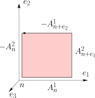
Figure 1: The plaquette variable $\Delta\theta_{n}^{3}=A^{2}_{n+e_{1}}-A^{2}_{n}-A^{1}_{n+e_{2}}+A^{1}_{n}$.

The classical (self-)duality of electromagnetic fields in the absence of sources (in vacuo) $E\rightarrow B,\ \ B\rightarrow-E$ is one of the oldest examples of a self-duality available. The bond algebra formalism gives insight into how this self-duality extends to non-compact vacuum QED. To see the connection with the self-duality we found for $\mathbb{Z}_{N}$ lattice gauge theories, we quantize electromagnetism in the axial gauge, $\phi\equiv 0$. In this gauge, the classical fields in terms of the vector potential $A$ are $E=-\frac{\partial A}{\partial t},\ \ \ B=\nabla\times A$. If we next apply canonical quantization to electromagnetism written in this gauge, we get vacuum QED in the form

$$H=\int d^{3}x\ \frac{1}{2}(\Pi^{2}+(\nabla\times A)^{2}),$$

together with canonical commutation relations $[A_{m}(x,t),\Pi_{l}(y,t)]=i\delta_{ml}\delta(x-y)$, where we made the canonical substitution $\frac{\partial A}{\partial t}=-E\rightarrow\Pi$. Furthermore, from gauge invariance, we have that the subspace of physical states (gauge invariant states) of the full Hilbert space is specified by the so called Gauss constraint: $\nabla\cdot\Pi\ |\mbox{physical}\rangle=0$ (physically, this means we only keep those states on which $\nabla\cdot E=0$). To investigate the bond algebra of this Hamiltonian, it is convenient to discretize the theory and consider it on a $d=3$ cubic lattice of lattice spacing $a$. The Hamiltonian then reads ($n=(n^{1},n^{2},n^{3})$)

$$H=\sum_{n}a^{3}\sum_{i=1}^{3}\frac{1}{2}(\Pi_{n}^{i})^{2}+\frac{1}{2}(\Delta\theta_{n}^{i})^{2},$$

where $[A_{n}^{i},\Pi_{m}^{k}]=i\delta^{ik}\delta_{n,m}$, and

$$\Delta\theta_{n}^{1}=(A^{3}_{n+e_{2}}-A^{3}_{n}-A^{2}_{n+e_{3}}+A^{2}_{n})/a$$

$$\Delta\theta_{n}^{2}=(A^{1}_{n+e_{3}}-A^{1}_{n}-A^{3}_{n+e_{1}}+A^{3}_{n})/a$$

$$\Delta\theta_{n}^{3}=(A^{2}_{n+e_{1}}-A^{2}_{n}-A^{1}_{n+e_{2}}+A^{1}_{n})/a$$

are the discretized form of the components of $\nabla\times A$. We call the interaction terms $\Delta\theta$ plaquette interactions, borrowing the terminology we used with $\mathbb{Z}_{N}$ gauge theories (see Fig. 1).

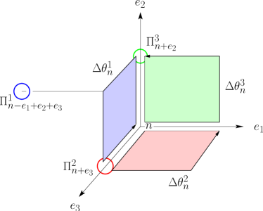
Figure 2: Schematic of the bond algebra mapping (13). Associated with each lattice site $n$, there are three $\Pi$ fields and three $\Delta\theta$ plaquettes. The $\Delta\theta$ plaquettes at site $n$ map by (13) to displaced $\Pi$s, each colored plaquette mapping to the $-\Pi$ at the correspondingly colored site.

The first thing to notice is that only four plaquette variables $\Delta\theta$ have non-trivial commutation relations with any given momentum component $\Pi^{i}_{n}$ at site $n$ and similarly, only four $\Pi$ fields have non-trivial commutation relations with any given $\Delta\theta^{i}_{n}$. Thus we have a good case for an automorphism that exchanges $\Pi\leftrightarrow\Delta\theta$. In fact, one such automorphism is given by

$$\Pi^{1}_{n}\mapsto\tilde{\Pi}^{1}_{n}=\Delta\theta^{1}_{n},\ \ \Delta\theta^{1}_{n}\mapsto\tilde{\Delta}\theta^{1}_{n}=-\Pi^{1}_{n-e_{1}+e_{2}+e_{3}}$$

$$\Pi^{2}_{n}\mapsto\tilde{\Pi}^{2}_{n}=\Delta\theta^{2}_{n-e_{1}+e_{2}},\ \ \Delta\theta^{2}_{n}\mapsto\tilde{\Delta}\theta^{2}_{n}=-\Pi^{2}_{n+e_{3}}$$ (13)

$$\Pi^{3}_{n}\mapsto\tilde{\Pi}^{3}_{n}=\Delta\theta^{3}_{n-e_{1}+e_{3}},\ \ \Delta\theta^{3}_{n}\mapsto\tilde{\Delta}\theta^{3}_{n}=-\Pi^{3}_{n+e_{2}}.$$

The geometry of this mapping is clarified in the Figs. 2 and 3. A moment’s reflection makes it clear that this mapping is nothing other than $E\mapsto B,\ B\mapsto-E$, the quantum descendant of the classical electromagnetic self-duality. As explained in the main body of our paper, the self-duality mapping serves the double purpose of establishing the existence of a self-duality and defining the dual variables. We have explicitly shown the dual variables above, naming them $\tilde{\Pi}$ and $\tilde{A}$. The dual vector potential is defined implicitly by the above relations, as, for instance, $\tilde{\Delta}\theta_{n}^{1}=(\tilde{A}^{3}_{n+e_{2}}-\tilde{A}^{3}_{n}-\tilde{A}^{2}_{n+e_{3}}+\tilde{A}^{2}_{n})/a$.

It is interesting to compute explicitly the dual variables in the continuum limit $a\rightarrow 0$, paralleling the discussion of dual variables for the scalar field given in the main body of this paper. In this limit, (13) implies the relations

$$\tilde{\Pi}(x,t)=\nabla\times A(x,t)$$

$$\nabla\times\tilde{A}(x,t)=-\Pi(x,t)$$

between the initial and the dual operator variables. Thus $\tilde{\Pi}$ is already explicitly given in terms of $A$. We need to solve the second relation for $\tilde{A}$. It is not difficult to check that, on physical states (on which $\nabla\cdot\Pi$ vanishes),

$$\tilde{A}(x,t)=-\frac{1}{4\pi}\nabla\times\int d^{3}w\ \frac{\Pi(w,t)}{|x-w|}.$$

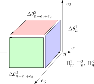
Figure 3: The effect of the exchange duality of (13) on the three $\Pi$ fields at site $n$.

References

• (1) R. Savit, Rev. Mod. Phys. 52, 453 (1980).
• (2) E. Witten, Phys. Today 50, 28 (1997).
• (3) H.A. Kramers and G.H. Wannier, Phys. Rev. 60, 252 (1941).
• (4) C.D. Batista and G. Ortiz, Phys. Rev. Lett. 86, 1082 (2001); Adv. in Phys. 53, 2 (2004).
• (5) Z. Nussinov and G. Ortiz, Phys. Rev. B 79, 214440 (2009).
• (6) We call an operator “irrelevant in the thermodynamic limit” when its expectation value in any state, divided by the system’s size, vanishes in this limit.
• (7) L.P. Kadanoff and H. Ceva, Phys. Rev. B 3, 3918 (1971).
• (8) J. B. Kogut, Rev. Mod. Phys. 51, 659 (1979).
• (9) Y. Tokura and N. Nagaosa, Science 288, 462 (2000).
• (10) Z. Nussinov and E. Fradkin, Phys. Rev. B 71, 195120 (2005).
• (11) C. Xu and J.E. Moore, Phys. Rev. Lett. 93, 047003 (2004).
• (12) S. A. Kivelson, D. S. Rokhsar, and J. P. Sethna, Phys. Rev. B 35, 8865 (1987); D. S. Rokhsar and S. A. Kivelson, Phys. Rev. Lett. 61, 2376 (1988).
• (13) G. ’t Hooft, Nuc. Phys. B 153, 141 (1979).
• (14) T. Yoneya, Nuc. Phys. B 144, 195 (1978).
• (15) G. Ortiz, Z. Nussinov, C. D. Batista, and E. Cobanera, to be published.
• (16) $K$ is computed from $\frac{1}{2}\frac{\partial F_{N}(K)}{\partial K}=e^{-\frac{1}{2g^{2}}(1-\cos\frac{2\pi}{N})}$, where $F_{N}(K)=\sum_{n=0}^{N-1}e^{2K\cos(\frac{2\pi}{N}n)}$; $K^{*}$ is $K$ at $g=g^{*}$ ortiz .
• (17) J. Jersak et. al., Phys. Rev. Lett. 77, 1933 (1996).
• (18) J. Frohlich and T. Spencer, Comm. Math. Phys. 81, 527 (1981).
• (19) A. M. Polyakov, Nucl. Phys. B 120, 429 (1977).
• (20) F. Y. Wu and Y. K. Wang, J. Math. Phys. 17, 439 (1976).

References

• (1) R. Savit, Rev. Mod. Phys. 52, 453 (1980).
• (2) A. Yu. Kitaev, Annals Phys. 303, 2 (2003).
• (3) I.S. Tupitsyn, A. Kitaev, N.V. Prokof’ev, and P.C.E. Stamp, cond-mat/08043175.
• (4) J. Vidal, S. Dusuel, and K. P. Schmidt, Phys. Rev. B 79, 033109 (2009).
• (5) F.J. Wegner, J. of Math. Phys. 12, 2259 (1971).
• (6) J. B. Kogut, Rev. Mod. Phys. 51, 659 (1979).
• (7) E. Fradkin and S. E. Shenker, Phys. Rev. D 19, 3682 (1979).
• (8) Z. Nussinov, Phys. Rev. D 72, 054509 (2005).
• (9) M. Blume, V. J. Emery, and R. B. Griffiths, Phys. Rev. A 4, 1071 (1971).
• (10) L. Mittag and M. J. Stephen, J. Math. Phys. 12, 441 (1971).
• (11) J.R. Baxter, Exactly Solved Models in Statistical Mechanics, Dover, 2007.
Refer to caption