A New Regularization of the One-Dimensional Euler and Homentropic Euler Equations

Abstract

This paper examines an averaging technique in which the nonlinear flux term is expanded and the convective velocities are passed through a low-pass filter. It is the intent that this modification to the nonlinear flux terms will result in an inviscid regularization of the homentropic Euler equations and Euler equations. The physical motivation for this technique is presented and a general method is derived, which is then applied to the homentropic Euler equations and Euler equations. These modified equations are then examined, discovering that they share the conservative properties and traveling wave solutions with the original equations. As the averaging is diminished it is proven that the solutions converge to weak solutions of the original equations. Finally, numerical simulations are conducted finding that the regularized equations appear smooth and capture the relevant behavior in shock tube simulations.

1 Introduction

This paper examines a modification of the homentropic Euler and Euler equations where flux term is expanded and the convective velocities are passed through a low-pass filter. It is the intent that this modification to the nonlinear flux terms will result in an inviscid regularization of the homentropic Euler equations and Euler equations. The ultimate goal with this regularization is to develop a proper modeling of small scale behavior so that both shocks and turbulence can be captured in one comprehensive technique. This paper primarily addresses the shock capturing capabilities of the developed technique.

The inspiration for this new technique comes from recent work done on a similarly modified Burgers equation. The Burgers equation, $u_{t}+uu_{x}=0$, is considered a simplistic model of compressible flow which forms shocks readily. Classically, this equation is regularized with a dissipative term, such as viscosity or hyper-viscosity. Additionally Burgers equations can be regularized with linear dispersion resulting in the KdV equations. Recently, work has been done by our group and others, investigating a regularization of the Burgers equations where the nonlinear term is manipulated by averaging the convective velocity [1, 2, 3, 4, 5, 6],

$$u_{t}+\bar{u}u_{x}=0$$ (1a)

$$\bar{u}=g^{\alpha}\ast u$$ (1b)

$$g^{\alpha}=\frac{1}{\alpha}g(\frac{x}{\alpha}),$$ (1c)

where $g$ is an averaging kernel with emphasis on the Helmholtz filter. In this paper we extend this technique to the homentropic Euler and Euler equations.

The technique used on the Burgers equations has been thoroughly investigated and been established as a valid shock regularization technique. It has been shown that solutions to Equations (1) exist and are unique [2, 3] for a wide variety of filters. This result has also been extended for a multiple dimensional version of the equations as well [2]. It has been shown that when the initial conditions are $C^{1}$, the solution remains $C^{1}$ for all time [2]. Furthermore, for bell shaped initial conditions it is proven that as the averaging approaches zero ($\alpha\to 0$), the solutions to Equation (1) converge to the entropy solution of inviscid Burgers equation [5]. There is also convincing evidence that this holds true for all continuous initial conditions [5]. These analytical results along with multiple numerical results regarding shock thickness and energy decay results show that this is a valid shock regularization technique.

The work on the regularization of the Burgers equation is inspired by and related to work done on the Lagrangian Averaged Navier-Stokes (LANS-$\alpha$) equations [7, 8, 9, 10, 11, 12, 13, 14]. The LANS-$\alpha$ equations also employ an averaged velocity in the nonlinear term and have been successful in modeling some turbulent incompressible flows.

It is thought that a regularization could be accomplished for the equations that describe compressible flow. Encouraged by the results for Burgers equation, the next step is to attempt to introduce averaging into the one-dimensional homentropic Euler equations, a simplified version of the full Euler equations, where pressure is purely a function of density. There have been several attempts at such a regularization.

Inspired by the existence uniqueness proofs from the averaged Burgers equations [2, 3], Norgard and Mohseni [15] averaged the characteristics of the homentropic Euler equations to derive the equations

$$\rho_{t}+\bar{u}\rho_{x}+\rho\frac{\bar{a}}{a}u_{x}=0$$ (2a)

$$u_{t}+\bar{u}u_{x}+\frac{a\bar{a}}{\rho}\rho_{x}=0$$ (2b)

$$\bar{u}=g\ast u$$ (2c)

$$\bar{a}=g\ast a$$ (2d)

with $a^{2}=\gamma\rho^{\gamma-1}.$ While these equations were proven to have a convenient existence and uniqueness proof, the equations were ultimately found to have significant departures in behavior from the homentropic Euler equations, specifically for the Riemann problem. What was discovered is that when the characteristics are averaged, there will be no creation or destruction of characteristics. A shock in homentropic Euler equations can produce new characteristics in one of the Riemann invariants. The new equations does not capture this behavior and results in departures from the desired behavior.

Using a Lagrangian averaging technique Bhat and Fetecau [16] derived the following equations

$$\rho_{t}+(\rho u)_{x}=0$$ (3)

$$w_{t}+(uw)_{x}-\frac{1}{2}(u^{2}+\alpha^{2}u_{x}^{2})_{x}=-\frac{p_{x}}{\rho}$$ (4)

$$\rho w=\rho v-\alpha^{2}\rho_{x}u_{x}$$ (5)

$$v=u-\alpha^{2}u_{xx}.$$ (6)

While the solutions to the system remained smooth and contained much structure it was found that the equations were “not well-suited for the approximation of shock solutions of the compressible Euler equations.”

Another attempt by Bhat, Fetecau, and Goodman used a Leray-type averaging [17] leading to the equations

$$\rho_{t}+\bar{u}\rho_{x}+\rho u_{x}=0$$ (7)

$$u_{t}+\bar{u}u_{x}+\frac{p_{x}}{\rho}=0$$ (8)

$$u=\bar{u}-\alpha^{2}\bar{u}_{xx}.$$ (9)

with $p=\kappa\rho^{\gamma}$. They then showed that weakly nonlinear geometrical optics (WNGO) asymptotic theory predicts the equations will have global smooth solutions for $\gamma=1$ and form shocks in finite time for any other value of $\gamma$; namely $\gamma\neq 1$.

Additionally in 2005, H. S. Bhat et. al. [18] applied the Lagrangian averaging approach to the full compressible Euler equations. Their approach successfully derived a set of Lagrangian Averaged Euler (LAE-$\alpha$) equations. However, these equations were quite long and complicated, and it seemed that numerical simulations involving these equations would be impractical for real world applications.

This paper examines another attempt at developing a regularization of the homentropic Euler and Euler equations with positive results thus far. Section 2 details the motivation behind the technique with section 4 detailing the general method. Section 3 specifies the averaging kernels that we consider in the regularizations. Section 6 examines the modified homentropic Euler equations looking at conservation of mass and momentum, traveling wave solutions, eigenvalues, convergence to weak solutions of the original homentropic Euler equations, and finally examining some numerical results. Section 7 examines the same properties, but with the modified Euler equations. All is then followed by concluding remarks.

2 Motivation

The motivation for our technique stems from a simple concept: that nonlinear terms generate high wave modes as continuously as time progresses. Consider the mechanics behind shock formation and turbulence. The nonlinear convective term $\mathbf{u}\cdot\triangledown\mathbf{u}$ generates high wave modes, by transferring energy into smaller scales as time progresses. This nonlinear term is found in the Burgers equations where it causes nonlinear steepening resulting in shocks. It is also found in the Euler and Navier-stokes equations where is generates high wave modes by tilting and stretching vortices [19]. Thus this nonlinear term is cascading energy down into smaller and smaller scales. In the 3D Navier-Stokes and 3D Euler equations, the energy cascade has a slope of -$\frac{5}{3}$ until the Kolmogorov scale, illustrated in figure 1a. The Burgers equation has an energy cascade slope of -$2$ until viscosity begins to dominate; seen in figure 1b [20, 21]. It is by reducing this cascade of energy after some scale that we intend to regularize the Euler equations. In the Burgers equation the nonlinear term $uu_{x}$ was replaced with $\bar{u}u_{x}$. A low pass filtered velocity will have less energy in its high wave modes after the scale $\frac{1}{\alpha}$. Thus when inserted into the nonlinear term, the energy cascade will be lessened. This modification to the Burgers equations was found to result in a regularization of the equations. It is our hypothesis that a similar modification to the Euler equations will have similar results.

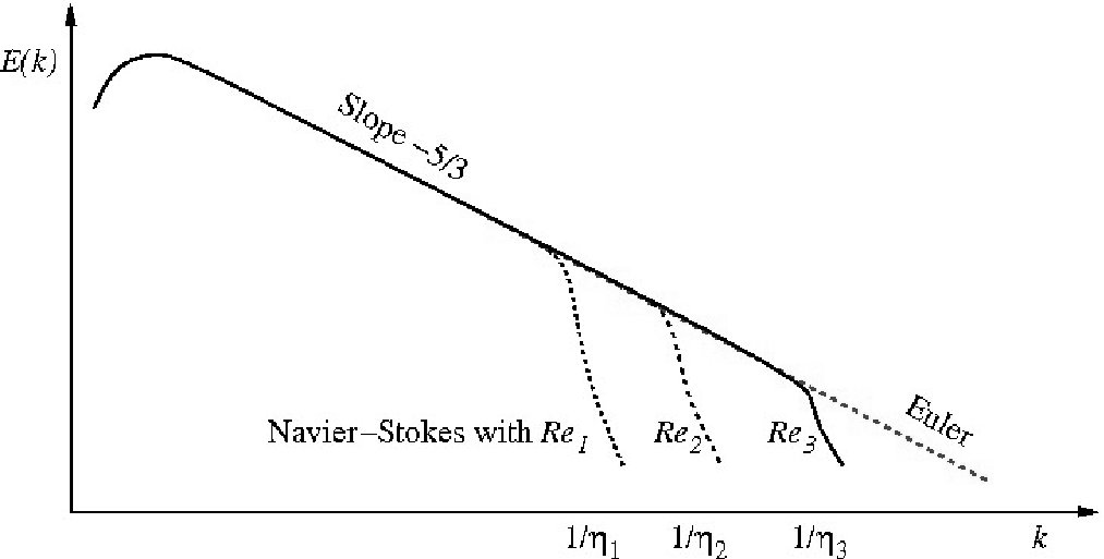
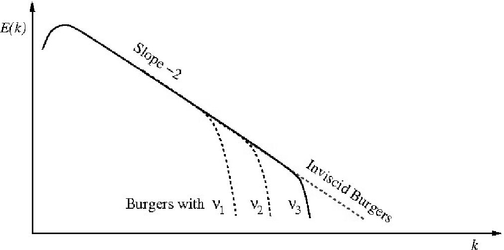
(a)

(b)

Figure 1: Schematics of energy cascade for the Navier-Stokes/Euler equations and the viscous/inviscid Burgers equation are shown. In an inviscid flow, both turbulence and shocks show continuous generation of higher wave modes indefinitely. (a) Energy cascades from high wavelengths to lower wavelengths at a predicted rate of -$\frac{5}{3}$ for the Navier-Stokes/Euler equations. For the Navier-Stokes equations, the kinetic energy drops drastically upon reaching a certain wavelength; the Kolmogorov scale, $\eta$. For the Euler equations the cascade continues on indefinitely. Here $Re_{1}<Re_{2}<Re_{3}$. (b) For the Burgers equation, shocks can form from continuous initial conditions. The energy cascade has a slope of -$2$ when shocks form, until viscosity begins to exert its influence and balance the steepening effect of the nonlinear term. Here $\nu_{3}<\nu_{2}<\nu_{1}$.

3 Averaging kernels

In our previous work, [2, 5] the low pass filters were assumed to have certain properties. Specifically the convolution kernels $g$ were assumed to be normalized, nonnegative, decreasing, and even. This is summarized in table 1. The physical rational behind these properties can be found in our previous work [2]. For this paper similar properties are assumed for the filters. However, only sections 4 and 5 deal with a general filter. All other sections deal exclusively with the Helmholtz filter which possesses all these characteristics. The Helmholtz filter is defined as

$$u=\bar{u}-\alpha^{2}\bar{u}_{xx},$$ (10)

and thus has an averaging kernel of

$$g^{\alpha}(x)=\frac{1}{2\alpha}\exp(-\frac{|x|}{\alpha}).$$ (11)

Table 1: This table succinctly lists the requirements of the low pass filters employed.

Properties	Mathematical Expression
Normalized	$\int g$=1
Nonnegative	$g(\mathbf{x})>0,\,\forall\mathbf{x}$
Decreasing	$|\mathbf{x}_{1}|\geq|\mathbf{x}_{2}|\Rightarrow g(\mathbf{x}_{1})\leq g(\mathbf{x}_{2})$
Symmetric	$|\mathbf{x}_{1}|=|\mathbf{x}_{2}|\Rightarrow g(\mathbf{x}_{1})=g(\mathbf{x}_{2})$

4 A general method

The successful regularization of the Burgers equations can be extended in several ways. As mentioned in the introduction, we had previously interpreted the CFB equations as an averaging of the characteristics [15]. Bhat, Fetecau, and Goodman interpreted the regularization of the Burgers equation as an averaging of the convective velocity, a Leray-type averaging [17]. Both of these interpretations, when extended to the homentropic Euler equations, have not led to the desired regularization of homentropic Euler equations. Here we examine yet another interpretation of the CFB equations, based on a conservation law perspective. This approach addresses the cascade of energy generated by the nonlinear terms. We then discuss how the technique used in regularizing the Burgers equation can be extend to a general technique to be used on conservation laws. Begin by looking at the inviscid Burgers equation

$$u_{t}+(uu)_{x}=0.$$ (12)

The flux term represents that the quantity $u$ is flowing into a control volume with velocity $u$. When the product rule is applied to the flux term the result is

$$u_{t}+uu_{x}+uu_{x}=0.$$ (13)

Each nonlinear term in the above equation results in steepening waves which cascades energy into higher wave modes. It is this energy cascade that produces shocks. In section 2, it was discussed how this cascade of energy can be reduced by filtering the convective velocity. Thus the non-differentiated term is passed through a low pass filter. The resulting equation is

$$u_{t}+\bar{u}u_{x}+\bar{u}u_{x}=0,$$ (14)

which has been referred to as the convectively filtered Burgers (CFB) equations. The portrayal of the CFB equations here differs from Equation (1) and in previous papers [1, 3, 4, 2, 5, 6] by a factor of 2, but is identical under rescaling.

Now we extend this technique to a more general method. Suppose there is a single or multiple conservation laws of the form

$$Q_{t}+(Qu)_{x}=0.$$ (15)

The proposed method is to apply the product rule to the nonlinear term and then apply a filter to the non-differentiated quantities. This results in

$$Q_{t}+\bar{Q}u_{x}+\bar{u}Q_{x}=0.$$ (16)

We believe that this filtering of the non-differentiated quantities will reduce the energy cascade and provide a regularization of the conservation law. It is this general method that we apply to the homentropic Euler and Euler equations.

5 Conservation of conserved quantities

Before we begin the examination of the modified homentropic Euler and Euler equations we will first examine how the modification of the nonlinear term still preserves the original conserved quantities. Again consider the more general conservation law

$$Q_{t}+(Qu)_{x}=0$$ (17)

and its regularized version

$$Q_{t}+\bar{Q}u_{x}+\bar{u}Q_{x}=0$$ (18a)

$$\bar{u}=g*u$$ (18b)

$$\bar{Q}=g*Q.$$ (18c)

Integrate $Q_{t}$ over the spatial domain and substitute Equations (18b) and (18c) and the full definition of convolution to obtain

$$\frac{\partial}{\partial t}\int Q(x)dx=-\int\int g(x-y)Q(y)u^{\prime}(x)\,dy\,dx-\int\int g(x-y)u(y)Q^{\prime}(x)\,dy\,dx.$$ (19)

Integrate by parts to obtain

$$\frac{\partial}{\partial t}\int Q(x)dx=\int\int g^{\prime}(x-y)\left(Q(y)u(x)+u(y)Q(x)\right)\,dy\,dx.$$ (20)

If $g$ is even, then $g^{\prime}$ is odd and $g^{\prime}(x-y)$ is anti-symmetric over $y=x$. Clearly $\left(Q(y)u(x)+u(y)Q(x)\right)$ is symmetric over $y=x$ and thus by symmetry

$$\frac{\partial}{\partial t}\int Q(x)dx=0.$$ (21)

From this it is determined the modified conservation law still conserves the original conserved quantity. Thus we see that the proposed method conserves the quantities that the original conservation laws were designed to preserve. This property is independent of the filter so long that it is even, which was a requirement of section 3.

6 The one-dimensional homentropic Euler equations

Examine the homentropic Euler equations

$$\rho_{t}+(\rho u)_{x}=0$$ (22a)

$$(\rho u)_{t}+(\rho uu+P)_{x}=0,$$ (22b)

with pressure defined as $P=\rho^{\gamma}$. Equation (22a) and (22b) are the mathematical expressions of conservation of mass and momentum respectively. The homentropic Euler equations makes the assumption that the entropy is constant throughout the entire domain and thus the pressure can be expressed solely as a function of the density [22]. This differs from the isentropic Euler equations where the entropy is constant along streamlines but not necessarily constant on the whole domain. It is found that the homentropic Euler equations are an accurate predictor of gas dynamics behavior for low pressure.

Both equations have a nonlinear term that fits the general method from section 4. Apply the method, break the nonlinear term apart, and then apply the filter to the non-differentiated terms in the nonlinear terms to obtain the equations

$$\rho_{t}+\bar{\rho}u_{x}+\bar{u}\rho_{x}=0$$ (23a)

$$(\rho u)_{t}+(\overline{\rho u})u_{x}+\bar{u}(\rho u)_{x}+P_{x}=0$$ (23b)

with pressure defined as $P=\rho^{\gamma}$. These equations are now referred to as the regularized homentropic Euler equations. For the following analysis, the only filter that is considered is the Helmholtz filter (10).

6.1 Conservation of mass and momentum

The homentropic Euler equations (22) are conservation laws for mass and momentum. These equations are reflections of important physical principles. In order to be physically relevant it is desirable that any regularization of the homentropic Euler equations would also preserve this structure. In section 5 we established that the technique used will preserve the conservative structure of the original equations. Here we reverify that result for the regularized homentropic Euler equations (23) by casting the equations into a conservative form using the Helmholtz filter.

Consider the regularized homentropic Euler equations

$$\rho_{t}+\bar{\rho}u_{x}+\bar{u}\rho_{x}=0$$ (24a)

$$(\rho u)_{t}+(\overline{\rho u})u_{x}+\bar{u}(\rho u)_{x}+P_{x}=0$$ (24b)

with

$$u=\bar{u}-\alpha^{2}\bar{u}_{xx}$$ (25a)

$$\rho=\bar{\rho}-\alpha^{2}\bar{\rho}_{xx}$$ (25b)

$$\rho u=\overline{\rho u}-\alpha^{2}\overline{\rho u}_{xx}.$$ (25c)

By substituting in Equations (25a), (25b), and (25c) and then regrouping the similar terms the regularized homentropic Euler equations can be rewritten as

$$\rho_{t}+\left(\bar{\rho}\bar{u}-\alpha^{2}(\bar{u}\bar{\rho}_{xx}+\bar{\rho}\bar{u}_{xx})+\alpha^{2}\bar{u}_{x}\bar{\rho}_{x}\right)_{x}=0$$ (26a)

$$(\rho u)_{t}+\left(\overline{\rho u}\bar{u}-\alpha^{2}(\bar{u}\overline{(\rho u)}_{xx}+\overline{\rho u}\bar{u}_{xx})+\alpha^{2}\bar{u}_{x}\overline{\rho u}_{x}+P\right)_{x}=0.$$ (26b)

This shows that the regularized homentropic Euler equations can be written in a conservative form and preserve both mass $\int\rho$ and momentum $\int\rho u$ as well as the averaged mass $\int\bar{\rho}$ and averaged momentum $\int\overline{\rho u}$. Examination of Equations (26) could lead to more geometric structure. They may also lead to the application of numerical techniques designed specifically for conservation laws.

6.2 Traveling wave solution

In this section, we establish that a previously known traveling wave solution to the homentropic Euler equations is in fact a traveling wave solution to the regularized homentropic Euler equations as well. The traveling wave solution that we examine for the homentropic Euler equations is a single traveling shock.

First we establish notation used in this section. The operator $\left[\cdot\right]$ will be used to quantify the difference between the right and left limits of a function at a discontinuity. For example if the limits of $u(x)$ at $x^{*}$ are defined as

$$\lim_{x\to x^{*+}}u(x)=u_{R}$$ (27)

$$\lim_{x\to x^{*-}}u(x)=u_{L},$$ (28)

then at $x^{*}$

$$\left[u\right]=u_{R}-u_{L}.$$ (29)

The Rankine-Hugoniot jump conditions establish that for weak solutions of conservation laws of the form

$$\textbf{Q}_{t}+(\textbf{f})_{x}=0$$ (30)

a traveling discontinuity must have a speed $S$, where $S$ is defined as [22]

$$S=\frac{[\textbf{f}]}{[\textbf{Q}]}.$$ (31)

Using this relationship it is easy to establish that the following is a weak solution to the homentropic Euler equations (22)

$$u=\left\{\begin{array}[]{ll}u_{L}&x<St\\ u_{R}&x\geq St\end{array}\right.$$ (34)

$$\rho=\left\{\begin{array}[]{ll}\rho_{L}&x<St\\ \rho_{R}&x\geq St\end{array}\right.$$ (37)

The speed of the shock $S$ is twice defined, once for each conservation law, by the Rankine-Hugoniot jump conditions as

$$S=\frac{[\rho u]}{[\rho]}$$ (38)

and

$$S=\frac{[\rho uu+P]}{[\rho u]}.$$ (39)

Thus $u_{L},u_{R},\rho_{L},$ and $\rho_{R}$ must satisfy the relationship

$$\frac{[\rho u]}{[\rho]}=S=\frac{[\rho uu+P]}{[\rho u]}.$$ (40)

Next we will establish that Equation (34) is also a weak solution to the regularized homentropic Euler equations (26). It is straightforward to establish that with $u$ defined as in Equation (34) and using the Helmholtz kernel definition Equation (11) that $\bar{u}$ and $\bar{\rho}$ are

$$\bar{u}=\left\{\begin{array}[]{ll}\frac{u_{R}-u_{L}}{2}\exp(\frac{x-St}{\alpha})+u_{L}&x<St\\ \frac{u_{L}-u_{R}}{2}\exp(-\frac{x-St}{\alpha})+u_{R}&x\geq St\end{array}\right.$$ (43)

$$\bar{\rho}=\left\{\begin{array}[]{ll}\frac{\rho_{R}-\rho_{L}}{2}\exp(\frac{x-St}{\alpha})+\rho_{L}&x<St\\ \frac{\rho_{L}-\rho_{R}}{2}\exp(-\frac{x-St}{\alpha})+\rho_{R}&x\geq St\end{array}\right.$$ (46)

Thus the values of $\bar{u}$ and $\bar{\rho}$ at $x=St$ are

$$\bar{u}(St,t)=\frac{u_{R}+u_{L}}{2}$$ (47)

$$\bar{\rho}(St,t)=\frac{\rho_{R}+\rho_{L}}{2}.$$ (48)

Additionally using the definition of the Helmholtz filter, $u=\bar{u}-\alpha^{2}\bar{u}_{xx}$, we find that

$$\left[u\right]=\left[\bar{u}\right]-\alpha^{2}\left[\bar{u}_{xx}\right].$$ (49)

Since $\bar{u}$ is continuous we establish that

$$\left[\bar{u}_{xx}\right]=-\frac{1}{\alpha^{2}}\left[u\right],$$ (50)

with the similar result

$$\left[\bar{\rho}_{xx}\right]=-\frac{1}{\alpha^{2}}\left[\rho\right].$$ (51)

Looking at the conservation form of the regularized homentropic Euler equations (26), the Rankine-Hugoniot jump conditions state that in order for Equation (34) to be a weak solution, that the speed of the discontinuity, $S$, must satisfy

$$S=\frac{[\bar{\rho}\bar{u}-\alpha^{2}(\bar{u}\bar{\rho}_{xx}+\bar{\rho}\bar{u}_{xx})+\alpha^{2}\bar{u}_{x}\bar{\rho}_{x}]}{[\rho]}$$ (52)

and

$$S=\frac{[\overline{\rho u}\bar{u}-\alpha^{2}(\bar{u}\overline{(\rho u)}_{xx}+\overline{\rho u}\bar{u}_{xx})+\alpha^{2}\bar{u}_{x}\overline{\rho u}_{x}+P]}{[\rho u]}.$$ (53)

Since $\bar{u},\bar{\rho},\bar{u}_{x},$ and $\bar{\rho}_{x}$ are continuous Equation (52) reduces to

$$S=\frac{-\alpha^{2}(\bar{u}[\bar{\rho}_{xx}]+\bar{\rho}[\bar{u}_{xx}])}{[\rho]}.$$ (54)

Substitute in Equations (50) and (51) to simplify further to

$$S=\frac{(\bar{u}[\rho]+\bar{\rho}[u])}{[\rho]}.$$ (55)

Now, by using Equations (47) and (48) and the definition of $[\cdot]$ one can obtain

$$S = \frac{\frac{1}{2}(u_{R}+u_{L})(\rho_{R}-\rho_{L})+\frac{1}{2}(\rho_{R}+\rho_{L})(u_{R}-u_{L})}{[\rho]}$$ (56)

$$= \frac{(\rho_{R}u_{R}-\rho_{L}u_{L})}{[\rho]}$$ (57)

$$= \frac{[\rho u]}{[\rho]},$$ (58)

which is identical to Equation (38). Similarly Equation (53) reduces to Equation (39). Thus for this specific example, the Rankine-Hugoniot jump conditions are identical for the homentropic Euler equations and the regularized homentropic Euler equations. This validates our claim that Equation (34) is a traveling weak solution for the regularized homentropic Euler equations.

6.3 Shock Thickness

With Equation (34) validated as a traveling weak solution for the regularized homentropic Euler equations, we establish an analytical result about shock thickness. Here the thickness of the shock is defined to be the length over which 90% of the amplitude change takes place, centered at the point of inflection.

Again we note that from Equation (34), and the kernel definition of the Helmholtz filter (11), the traveling wave solution is

$$\bar{u}=\left\{\begin{array}[]{ll}\frac{u_{R}-u_{L}}{2}\exp(\frac{x-St}{\alpha})+u_{L}&x<St\\ \frac{u_{L}-u_{R}}{2}\exp(-\frac{x-St}{\alpha})+u_{R}&x\geq St\end{array}\right.$$ (61)

$$\bar{\rho}=\left\{\begin{array}[]{ll}\frac{\rho_{R}-\rho_{L}}{2}\exp(\frac{x-St}{\alpha})+\rho_{L}&x<St\\ \frac{\rho_{L}-\rho_{R}}{2}\exp(-\frac{x-St}{\alpha})+\rho_{R}&x\geq St\end{array}\right.$$ (64)

The thickness of the shock will then be $2\alpha b$, where b is the value where

$$\int_{-b}^{b}\frac{1}{2}exp(-|x|)\,dx=\int_{-\alpha b}^{\alpha b}\frac{1}{2\alpha}exp(\frac{-|x|}{\alpha})\,dx=0.9.$$ (65)

This length is independent of $\rho_{R},\rho_{L},u_{R}$ and $u_{L}$. As such, the thickness of the shock varies linearly on the parameter $\alpha$.

6.4 Diagonalization and eigenvalues

The homentropic Euler equations have very clearly defined eigenvalues, $u\pm a,$ where $a^{2}=\gamma\rho^{\gamma-1}$ is the speed of sound. This section examines how the proposed averaging affects the eigenvalues of the system and thus the characteristic speeds. In order to cast the equations in vector matrix form we first rewrite the equations in their primitive variable form

$$\rho_{t}+\bar{\rho}u_{x}+\bar{u}\rho_{x}=0$$ (66a)

$$u_{t}+\bar{u}u_{x}+\underbrace{\left(\frac{\overline{\rho u}-u\bar{\rho}}{\rho}\right)}_{\beta}u_{x}+\frac{\gamma\rho^{\gamma-1}}{\rho}\rho_{x}=0.$$ (66b)

The equations can then be written in vector matrix form leading to

$$\left[\begin{array}[]{c}\rho\\ u\\ \end{array}\right]_{t}+\underbrace{\left[\begin{array}[]{cc}\bar{u}&\bar{\rho}\\ \frac{a^{2}}{\rho}&\bar{u}+\beta\\ \end{array}\right]}_{A}\left[\begin{array}[]{c}\rho\\ u\\ \end{array}\right]_{x}=0.$$ (67)

The eigenvalues of matrix $A$ are

$$\lambda^{\pm}=\bar{u}+\frac{\beta}{2}\pm\sqrt{\frac{\beta^{2}}{4}+a^{2}\frac{\bar{\rho}}{\rho}}.$$ (68)

Examining quantities $\beta$ and $\frac{\bar{\rho}}{\rho}$ it seems apparent that as the filtering decreases $\beta\to 0$ and $\frac{\bar{\rho}}{\rho}\to 1$, thus regaining the original eigenvalues.

The matrix $A$ can as be diagonalized and can thus be written in the form

$$A=Q\Lambda Q^{-1}$$ (69)

where $\Lambda$ is a diagonal matrix with its diagonal entries being $\lambda^{\pm}$. Using this we can write the regularized homentropic Euler equations in the characteristic form

$$\frac{\partial\mathbf{v}}{\partial t}+\Lambda\frac{\partial\mathbf{v}}{\partial x}=0$$ (70)

where

$$d\mathbf{v}=Q^{-1}\left[\begin{array}[]{c}d\rho\\ du\\ \end{array}\right].$$ (71)

By diagonalizing $A$ we find that

$$Q^{-1}=\left[{\begin{array}[]{rc}1&{\displaystyle\frac{\rho\,\beta+\sqrt{\rho\,(\rho\,\beta^{2}+4\,a^{2}\,\mathit{\bar{\rho}})}}{2\,a^{2}}}\\[8.61108pt] 1&{\displaystyle\frac{\rho\,\beta-\sqrt{\rho\,(\rho\,\beta^{2}+4\,a^{2}\,\mathit{\bar{\rho}})}}{2\,a^{2}}}\end{array}}\right].$$ (72)

And thus we can define the quantities $v^{\pm}$ through the relation

$$dv^{\pm}=d\rho+\frac{\rho\,\beta\pm\sqrt{\rho\,(\rho\,\beta^{2}+4\,a^{2}\,\bar{\rho})}}{2\,a^{2}}\,du.$$ (73)

We can then say that $dv^{\pm}=0$ along the characteristic $dx=\lambda^{\pm}\,dt.$

If $\alpha=0$, there would be no filtering and $\beta=0$. In this case we would get

$$dv^{\pm}=d\rho\pm\frac{\rho}{a}du=0\quad\mbox{ along the characteristic }dx=u\pm a\,dt.$$ (74)

which is the case for the homentropic Euler equations. For the homentropic Euler equations the characteristic variables are able to be computed analytically and are

$$v^{\pm}=u\pm\frac{2a}{\gamma-1}.$$ (75)

For non-zero $\alpha$’s there appears to be no straightforward way of integrating Equation (73). Thus currently we have no analytical expression for the characteristic variables, though we have not spent much time investigation this possibility.

6.5 Convergence to a weak solution

It is the goal of our technique to develop new equations that effectively capture the low wave mode behavior of the original equations. Thus it is desirable that the regularized homentropic Euler equations approximate the homentropic Euler equations well. Ideally we can show that as the amount of filtering decreases we regain the original equations. One crucial step in determining this is proving that as $\alpha\to 0$ the solutions to the regularized homentropic Euler equations converge to a weak solution of the homentropic Euler equations. This, among other things, proves that as $\alpha\to 0$, the shocks produced by the regularized homentropic Euler equations travel at the same speed as those of the homentropic Euler equations, which is desirable.

As of yet, we have not been able to extend our existence theorems of the regularized Burgers equations (1) to the regularized homentropic Euler equations (23). Without this theorem we are forced to make several assumptions that we consider modest, considering the numerical evidence presented in section 6.7. We assume that for every $\alpha>0$ there exists a solution to Equations (24). Beyond that it is assumed that a subsequence of those solutions converge in $L^{1}_{loc}$ and the solutions are bounded independent of $\alpha.$ The following summarizes these assumptions.

$$||u||_{\infty}<U$$ (76a)

$$||\rho||_{\infty}<R$$ (76b)

$$\lim_{\alpha\to 0}u=\tilde{u}\mbox{ in }L^{1}_{loc}$$ (76c)

$$\lim_{\alpha\to 0}\rho=\tilde{\rho}\mbox{ in }L^{1}_{loc}$$ (76d)

With these assumptions we are able to prove that the solutions to the regularized homentropic Euler equations (23) will converge to weak solutions of the homentropic Euler equations (22). The examination of the claim is done with the Helmholtz filter, with $\bar{u}$ defined as

$$\bar{u}=u\ast g^{\alpha}$$ (77)

with

$$g(x)=\frac{1}{2}exp(-|x|)$$

and thus

$$g^{\alpha}(x)=\frac{1}{2\alpha}exp(-\frac{|x|}{\alpha}).$$

The unfiltered and filtered velocities can also be related by

$$u=\bar{u}-\alpha^{2}\bar{u}_{xx}.$$ (78)

Both definitions are used. The following bounds are easily established by examining the kernel.

$$||g||_{1}=1$$

and

$$\left|\left|\frac{\partial}{\partial x}g\right|\right|_{1}=1,$$

and thus

$$\left|\left|\frac{\partial}{\partial x}g^{\alpha}\right|\right|_{1}=\frac{1}{\alpha}.$$

These bounds combined with Young’s inequality [23] and the assumptions (76) give the following estimates

$$||\bar{u}||_{\infty}<U$$ (79)

$$||\bar{\rho}||_{\infty}<R$$ (80)

$$||\overline{\rho u}||_{\infty}<UR$$ (81)

$$||\bar{u}_{x}||_{\infty}<\frac{1}{\alpha}U$$ (82)

$$||\bar{\rho}_{x}||_{\infty}<\frac{1}{\alpha}R$$ (83)

$$||\overline{\rho u}_{x}||_{\infty}<\frac{1}{\alpha}UR$$ (84)

Along with these estimates, the last piece needed is taken from Duoandikoetxea [24]. The following lemma is a restatement of Duoandikoetxea’s Theorem 2.1 from page 25.

Lemma 6.1

Let $g$ be an integrable function on $\mathbb{R}$ such that $\int g=1$. Define $g^{\alpha}=\frac{1}{\alpha}g(\frac{x}{\alpha})$. Then

$$\lim_{\alpha\to 0}||g^{\alpha}\ast f-f||_{p}=0$$

if $f\in L^{p},1\leq p<\infty$ and uniformly (i.e. when $p=\infty$) if $f\in C_{0}(\mathbb{R})$.

With lemma 6.1 the convergence to weak solutions can now be proven. Begin by multiplying Equations (26) by a test function $\phi$ and integrate over time and space. It is assumed that $\phi$ has an infinite number of bounded and continuous derivatives and is compactly supported. Doing this we obtain the equations

$$\int_{\mathbb{R}}\int_{0}^{T}\rho_{t}\phi+\left(\bar{\rho}\bar{u}-\alpha^{2}(\bar{u}\bar{\rho}_{xx}+\bar{\rho}\bar{u}_{xx})+\alpha^{2}\bar{u}_{x}\bar{\rho}_{x}\right)_{x}\phi\,dt\,dx=0$$ (85a)

$$\int_{\mathbb{R}}\int_{0}^{T}(\rho u)_{t}\phi+\left(\overline{\rho u}\bar{u}-\alpha^{2}(\bar{u}\overline{(\rho u)}_{xx}+\overline{\rho u}\bar{u}_{xx})+\alpha^{2}\bar{u}_{x}\overline{\rho u}_{x}\right)+P)_{x}\phi\,dt\,dx=0.$$ (85b)

Integrate by parts to obtain

$$\int_{\mathbb{R}}\int_{0}^{T}\rho\phi_{t}+\left(\bar{\rho}\bar{u}\right)\phi_{x}\,dt\,dx=\int_{\mathbb{R}}\int_{0}^{T}\left(\alpha^{2}(\bar{u}\bar{\rho}_{xx}+\bar{\rho}\bar{u}_{xx})-\alpha^{2}\bar{u}_{x}\bar{\rho}_{x}\right)\phi_{x}\,dt\,dx$$ (86a)

$$\int_{\mathbb{R}}\int_{0}^{T}(\rho u)\phi_{t}+\left(\overline{\rho u}\bar{u}+P\right)\phi_{x}\,dt\,dx=\int_{\mathbb{R}}\int_{0}^{T}\left(\alpha^{2}(\bar{u}\overline{(\rho u)}_{xx}+\overline{\rho u}\bar{u}_{xx})-\alpha^{2}\bar{u}_{x}\overline{\rho u}_{x}\right))\phi_{x}\,dt\,dx.$$ (86b)

Clearly if the right hand side of Equations (86a) and (86b) limit to zero then the limit of $\rho$ and $u$ is a weak solution to the homentropic Euler equations. Begin by examining the term

$$\int_{\mathbb{R}}\int_{0}^{T}\alpha^{2}\bar{u}\bar{\rho}_{xx}\phi_{x}\,dt\,dx$$ (87)

Substitute the definition of the averaging so that $\alpha^{2}\bar{\rho}_{xx}=\bar{\rho}-\rho$ and examine the quantity

$$\int_{\mathbb{R}}\int_{0}^{T}\bar{u}(\bar{\rho}-\rho)\phi_{x}\,dt\,dx.$$ (88)

It was established that $\bar{u}$ and $\phi_{x}$ are bounded and by lemma 6.1 $(\bar{\rho}-\rho)$ converges in $L^{1}$ to zero. Thus we find

$$\lim_{\alpha\to 0}\int_{\mathbb{R}}\int_{0}^{T}\alpha^{2}\bar{u}\bar{\rho}_{xx}\phi_{x}\,dt\,dx=\int_{\mathbb{R}}\int_{0}^{T}\bar{u}(\bar{\rho}-\rho)\phi_{x}\,dt\,dx=0,$$ (89)

and the similar terms can be treated likewise.

Next examine the term

$$\int_{\mathbb{R}}\int_{0}^{T}\alpha^{2}\bar{u}_{x}\overline{\rho u}_{x}\phi_{x}\,dt\,dx.$$ (90)

Perform an integration by parts to obtain

$$-\int_{\mathbb{R}}\int_{0}^{T}\alpha^{2}\bar{u}\overline{(\rho u)}_{xx}\phi_{x}\,dt\,dx-\int_{\mathbb{R}}\int_{0}^{T}\alpha^{2}\bar{u}\overline{\rho u}_{x}\phi_{xx}\,dt\,dx.$$ (91)

The first term in Equation (91) limits to zero from the steps shown above. The second term can be bounded with the estimates found from Young’s inequality.

$$\left|\left|\int_{\mathbb{R}}\int_{0}^{T}\alpha^{2}\bar{u}\overline{\rho u}_{x}\phi_{xx}\,dt\,dx\right|\right| \leq\int_{\mathbb{R}}\int_{0}^{T}\alpha^{2}U\frac{1}{\alpha}UR|\phi_{xx}|\,dt\,dx$$ (92)

$$=\alpha U^{2}R||\phi_{xx}||_{1}$$ (93)

and thus limits to zero. The similar terms can be treated likewise. Thus we see that solutions to Equations (26) converge to weak solutions of the homentropic Euler equations as $\alpha\to 0$.

6.6 Numerics

In this section, we discuss the numerical techniques we used to simulate the regularized homentropic Euler equations and the homentropic Euler equations. Since the regularized homentropic Euler equations appear to be regularized and its solutions are smooth, we are able to use a pseudo-spectral method. The homentropic Euler equations tend to form shocks, so we use well-established techniques to handle this behavior.

6.6.1 Numerical simulations of the regularized homentropic Euler equations

For the regularized homentropic Euler equations, much like in turbulence simulation, we wish only to resolved the averaged quantities in our numerical simulations. To obtain the equations with only the smooth variables, we first apply the Helmholtz filter to Equations (23) and add $(\bar{\rho}\bar{u})_{x}$ or $(\overline{\rho u}\bar{u})_{x}$ to both sides.

$$\bar{\rho}_{t}+\left(\bar{\rho}\bar{u}\right)_{x}=\left(\bar{\rho}\bar{u}\right)_{x}-\overline{(\bar{\rho}u_{x}+\bar{u}\rho_{x})}$$ (94a)

$$\overline{\rho u}_{t}+\left(\overline{\rho u}\bar{u}+\bar{P}\right)_{x}=\left(\overline{\rho u}\bar{u}\right)_{x}-\overline{(\overline{\rho u}u_{x}+\bar{u}(\rho u)_{x})}.$$ (94b)

Then use the definition of the Helmholtz filter (10) to manipulate the equations to

$$\bar{\rho}_{t}+\left(\bar{\rho}\bar{u}\right)_{x}=\overline{(1-\alpha^{2}\partial_{x}^{2})\left(\bar{\rho}\bar{u}\right)_{x}-\bar{\rho}(\bar{u}_{x}-\alpha^{2}\bar{u}_{xxx})-\bar{u}(\bar{\rho}_{x}-\alpha^{2}\bar{\rho}_{xxx})}$$ (95a)

$$\overline{\rho u}_{t}+\left(\overline{\rho u}\bar{u}+\bar{P}\right)_{x}=\overline{(1-\alpha^{2}\partial_{x}^{2})\left(\overline{\rho u}\bar{u}\right)_{x}-\overline{\rho u}(\bar{u}_{x}-\alpha^{2}\bar{u}_{xxx})-\bar{u}((\overline{\rho u})_{x}-\alpha^{2}(\overline{\rho u})_{xxx})}.$$ (95b)

One can then simplify to obtain

$$\bar{\rho}_{t}+\left(\bar{\rho}\bar{u}\right)_{x}=-3\alpha^{2}\overline{(\bar{u}_{x}\bar{\rho}_{x})_{x}}$$ (96a)

$$\overline{\rho u}_{t}+\left(\overline{\rho u}\bar{u}+\bar{P}\right)_{x}=-3\alpha^{2}\overline{(\bar{u}_{x}\overline{\rho u}_{x})_{x}}.$$ (96b)

The equations are now fully in terms of the averaged quantities with the right hand side being the regularizing terms.

In order to reduce the potential for numerical dissipation we use a pseudo-spectral method to solve Equations (96). We advance the equations in time with an explicit, Runge-Kutta-Fehlberg predictor/corrector (RK45) [6]. The initial time step is chosen small enough to achieve stability, and is then varied by the code using the formula

$$h_{i+1}=\gamma h_{i}\left(\frac{\varepsilon h_{i}}{||\bar{\rho}_{i}-\hat{\rho}_{i}||_{2}}\right)^{\frac{1}{4}}.$$ (97)

Thus the new time step is chosen from the previous time step and the amount of error between the predicted density, $\bar{\rho}$ and the corrected density $\hat{\rho}$. The relative error tolerance was chosen at $\varepsilon=10^{-4}$ and the safety factor $\gamma=0.9$. If the new time step chosen was found to violate the CFL condition the time step was chosen according to the velocity speed and the speed of sound with CFL number $0.5$.

Spatial derivatives and the inversion of the Helmholtz operator were computed in the Fourier domain. The terms were converted into the Fourier domain using a Fast Fourier Transform, multiplied by the appropriate term and then converted back into the physical domain.

A number of high resolution simulations were done at the resolution of $2^{14}=65536$ grid points on the domain $[0,2\pi]$. We found that some long term simulations may suffer from long term numerical instabilities. After approximately 10,000 time steps, we would notice energy building up in the high wave modes near the resolution boundary. If not checked, these would contaminate the results of lower wave modes. In order to control this long term instability, every 200 time steps we zero out all the wave modes with wave number higher that $\frac{N}{3}$ where $N$ is the highest Fourier wave mode simulated. Wave modes higher than $\frac{2N}{3}$, are set to zero at every nonlinear multiplication to prevent aliasing. Numerical runs were conducted for values $\alpha=0.10,0.09,...,0.02,0.01.$ In the worst case scenario, $\alpha=0.01,$ the wave modes that are zeroed are over an order of magnitude higher than $\frac{1}{\alpha}$, as seen in figure 2.

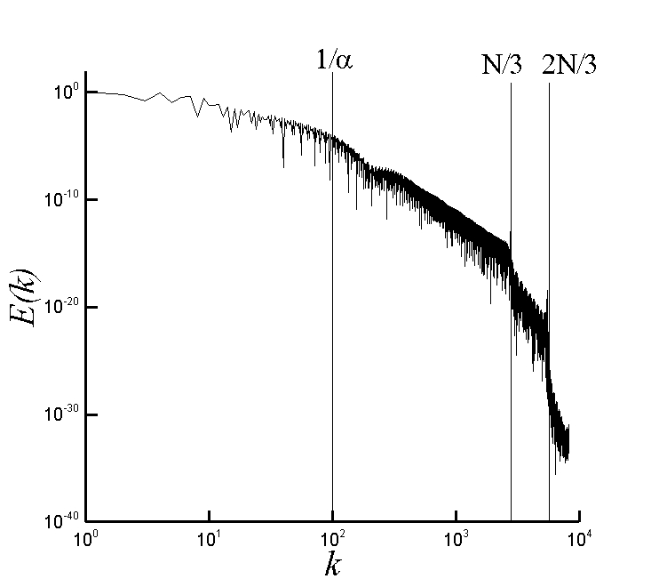
Figure 2: The spectral energy of $u$. The vertical lines represent three significant wave numbers. From left to right the lines represent $\frac{1}{\alpha}$, $\frac{N}{3}$, and $\frac{2N}{3}$, where $N$ is the highest Fourier wave mode simulated. The wave mode $\frac{N}{3}$ is the highest wave mode that is ever zeroed out in the simulations. Here with $\alpha=0.01$ you can see that zeroing of wave modes takes place an order of magnitude higher than where the filtering has its effect. This graph was taken from simulations of examples problem 105. Here $t=0.1$, $N=2^{13}$, and $n=2^{14}$, where $N$ is the number of Fourier modes resolved and $n$ is the number of grid points.

We attribute this error to the right hand side of Equations (96) for the following reasons. Examine the term

$$-3\alpha^{2}\overline{(\bar{u}_{x}\bar{\rho}_{x})_{x}}.$$ (98)

Expand the term to

$$-3\alpha^{2}\overline{\bar{u}_{xx}\bar{\rho}_{x}+\bar{u}_{x}\bar{\rho}_{xx}}.$$ (99)

and specifically notice the $\bar{u}_{x}\bar{\rho}_{xx}$ term. This term can be considered as a viscosity-like term that changes signs with $\bar{u}_{x}$. Now along the expansion wave $\bar{u}_{x}>0$ and thus there is a negative second derivative or viscosity-like term. Negative viscosity is inherently unstable, so we attribute the numerical instabilities to this. This is similar to the backscatter of energy to larger scales that is observed in turbulence.

6.6.2 Numerics for the homentropic Euler equations

For the numerical simulations of the homentropic Euler equations there are many established, available techniques[22]. We chose to use the Richtmyer method, a well-established if low order method, was utilized as described by [22]. This method is a second-order, finite-difference scheme and employs an artificial viscosity. This method requires an artificial viscosity for stability when examining the Riemann problem. Several different values of $\nu$ were tested to see that the value did not significantly affect the solutions on the time interval examined. For the numerical simulations shown here, the artificial viscosity was set at $\nu=0.08$. For reference, the simulations were done with $2^{14}$ grid points on a $[0,2\pi]$ domain.

6.7 Numerical results

This section examines some numerical simulations performed on Equations (96) with the technique described in the previous section. A shock tube or Riemann problem exhibits both shocks and expansion waves, some of the key behaviors of the homentropic Euler equations. Our pseudo-spectral method enforces periodic boundary conditions, so we created two pressure jumps in the initial conditions resolving this issue. Thus essentially a double shock tube problem is considered where there are two discontinuities in the initial conditions to make the left and right side boundary conditions identical. The example problem considered is

$$u_{0}(x)= 0$$ (100)

$$a_{0}(x)= \left\{\begin{array}[]{ll}1&0<x\leq\frac{2\pi}{3}\\ 2&\frac{2\pi}{3}<x\leq\frac{4\pi}{3}\\ 1&\frac{4\pi}{3}<x\leq 2\pi\end{array}\right.$$ (104)

which for $\gamma=1.4$, the constant for air, is equivalent to

$$u_{0}(x)= 0$$ (105)

$$\rho_{0}(x)= \left\{\begin{array}[]{ll}0.43120&0<x\leq\frac{2\pi}{3}\\ 13.7984&\frac{2\pi}{3}<x\leq\frac{4\pi}{3}\\ 0.43120&\frac{4\pi}{3}<x\leq 2\pi\end{array}\right..$$ (109)

In our previous work, we established that for the CFB equations (1) initial conditions with discontinuities were excluded in order to avoid non-entropic behavior [5]. By regularizing the initial conditions it was proven that the solution to the CFB equations would be regularized for all time. This was done by averaging the initial conditions with the same filter used on the velocity. We use this same approach here. Thus when the filter is applied to the entire equations to obtain Equations (96), the initial conditions are filtered twice with the same filter used on the equations.

In the simulation of the double shock tube problem the regularized homentropic Euler equations are displaying similar behavior to the homentropic Euler equations. Figures 3 and 4 show the solutions to the two sets of equations imposed on each other. One can see that the solutions to the regularized homentropic Euler equations capture both the expansion wave and the shock front. The solutions to the regularized homentropic Euler equations are seen to be smooth with the solutions tightening to the solutions of the homentropic Euler equations as $\alpha$ decreases.

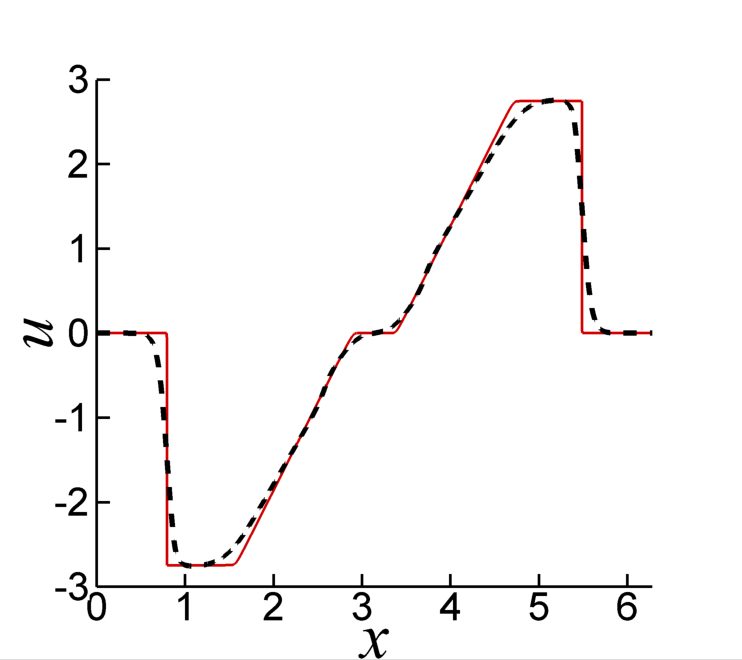
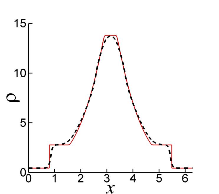
(a)

(b)

Figure 3: This figure shows a numerical simulation of the regularized homentropic Euler equations (dashed line) plotted against the solution to the homentropic Euler equations (solid line). Here the value of $\alpha=0.05$. In both figures, it is clear that the regularized homentropic Euler equations are capturing both the expansion wave and shock behavior. (a) The velocity. (b) The density.

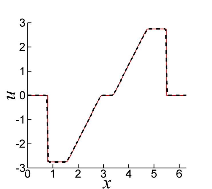
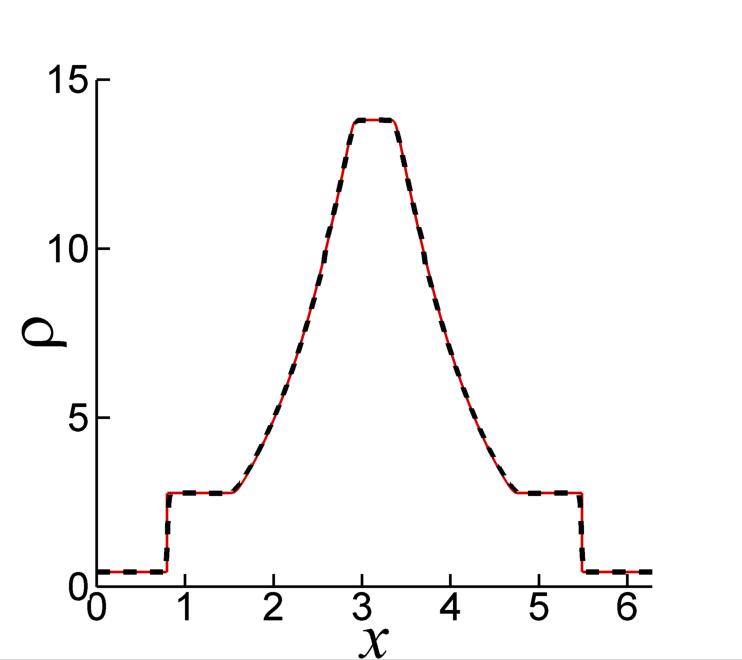
(a)

(b)

Figure 4: This figure shows a numerical simulation of the regularized homentropic Euler equations (dashed line) plotted against the solution to the homentropic Euler equations (solid line). Here the value of $\alpha=0.01$. In both figures, it is clear that the regularized homentropic Euler equations are capturing both the expansion wave and shock behavior. With the lower value of $\alpha$ the fit is much closer. (a) The velocity. (b) The density.

Now we check the convergence of the solutions of the regularized homentropic Euler equations to the solution of the homentropic Euler equations as $\alpha\to 0$. Figures 5 and 6 show that as $\alpha\to 0$ the error in the $L^{1}$ norm appears to be approaching zero for the example problem. This suggests that the solutions of the regularized homentropic Euler equations converge to the solutions of the homentropic Euler equations.

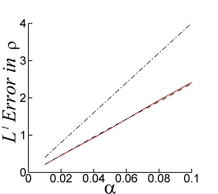
Figure 5: This figure displays the difference between the density in solutions of the regularized homentropic Euler equations and the solution of the homentropic Euler equations in the $L^{1}$ norm as $\alpha\to 0$. As $\alpha\to 0$ the difference in the solutions also approaches zero. The measurements were taken for $\alpha=0.01,0.02,...,0.1$ at times $t=0$,                        , $t=0.2$   , and $t=0.4$                .

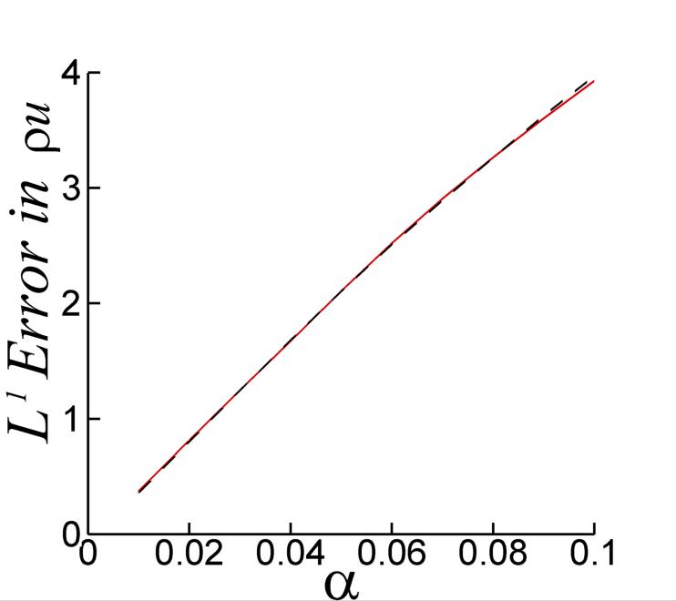
Figure 6: This figure displays the difference between the momentum in solutions of the regularized homentropic Euler equations and the solution of the homentropic Euler equations in the $L^{1}$ norm as $\alpha\to 0$. As $\alpha\to 0$ the difference in the solutions also approaches zero. The measurements were taken for $\alpha=0.01,0.02,...,0.1$ at times $t=0.2$   , and $t=0.4$                .

6.8 Kinetic energy rates

In addition to checking solution profiles, we examine the effect that our regularization technique has upon the kinetic energy. For the homentropic Euler equations we define kinetic energy as $\frac{1}{2}\rho u^{2}.$ For the regularized homentropic Euler equations there are three different averaged quantities, $\bar{\rho}$, $\bar{u}$, and $\overline{\rho u}$. With these quantities, kinetic energy can be defined in a variety of ways. In this section we examine a kinetic energy with unfiltered terms, $\frac{1}{2}\rho u^{2}$, and a kinetic energy with filtered terms, $\frac{1}{2}\bar{\rho}\bar{u}^{2}$. We have also examined the possible kinetic energies $\frac{1}{2}\overline{\rho u}\bar{u}$ and $\frac{\overline{\rho u}^{2}}{2\bar{\rho}}$, but for the example we are considering the difference between them and $\frac{1}{2}\bar{\rho}\bar{u}^{2}$ was of the order $10^{-14}$ and thus negligible. For flows with more small scale behavior, we would expect this difference to be more significant.

For the shock tube problem, the kinetic energy of the system clearly starts at zero. For the homentropic Euler equations the solution is self similar, depending only on the variable $\frac{x}{t}$. Thus the kinetic energy for the homentropic Euler equations will be a linear function of time. This can be seen in figure 7. We find that the energies of the regularized homentropic Euler equations mimic that of the homentropic Euler equations. In the simulations of the regularized homentropic Euler equations there is a brief period where the energy growth is curved before it appears to behave linearly. We attribute this to the averaging of the initial conditions. As we would expect, as $\alpha$ decreases the energies grow closer to those of the homentropic Euler equations.

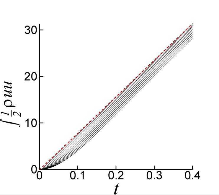
(a)

(b)

Figure 7: The kinetic energy of the homentropic Euler equations and the regularized homentropic Euler equations. The energy for the true solution of the homentropic Euler equations is shown as a dashed red line. The simulation of the regularized homentropic Euler equations for $\alpha=0.01,0.02,...,0.1$ are shown as solid black lines. The bottommost line represents $\alpha=0.1$. As $\alpha$ decreases the energy approaches the energy of the homentropic Euler equations. (a) These are plots of the unfiltered kinetic energies, $\frac{1}{2}\rho u^{2}$. (b) These are plots of the filtered kinetic energies, $\frac{1}{2}\bar{\rho}\bar{u}^{2}$. When examined the plots of $\frac{1}{2}\overline{\rho u}\bar{u}$ and $\frac{\overline{\rho u}^{2}}{2\bar{\rho}}$ were identical to this one.

7 The one-dimensional Euler equations

While the homentropic Euler equations are good for low pressures, to have real impact we want our technique to be able to capture the behavior of the full one-dimensional Euler equations. With the regularized homentropic Euler equations showing promise, we attempt to use the same general methodology on the one-dimensional Euler equations. The one-dimensional Euler equations consist of three conservation laws paired with a constitutive law. The conservation laws are conservation of mass, momentum, and energy. For the constitutive law, this paper is considering an ideal gas. Thus the one-dimensional Euler equations considered, in conservation form, are

$$\rho_{t}+(\rho u)_{x}=0$$ (110a)

$$(\rho u)_{t}+(\rho uu+P)_{x}=0$$ (110b)

$$(\rho e)_{t}+(\rho eu+uP)_{x}=0$$ (110c)

$$P=(\gamma-1)\left(\rho e-\frac{1}{2}\rho u^{2}\right)$$ (110d)

The technique described in section 4 applies the product rule to nonlinear terms and then the non-differentiated quantities are spatially filtered. Again this is to reduce the production of higher wave modes as time progresses, although as in the regularized homentropic Euler equations, we will see that an artificial viscosity is needed for numerical stability. When our averaging technique is applied, the new equations are

$$\rho_{t}+\bar{\rho}u_{x}+\bar{u}\rho_{x}=0$$ (111a)

$$(\rho u)_{t}+\overline{\rho u}u_{x}+\bar{u}(\rho u)_{x}+P_{x}=0$$ (111b)

$$(\rho e)_{t}+\overline{\rho e}u_{x}+\bar{u}(\rho e)_{x}+\overline{P}u_{x}+\bar{u}P_{x}=0$$ (111c)

$$P=(\gamma-1)\left(\rho e-\frac{1}{2}\rho u^{2}\right)$$ (111d)

which we refer to as regularized Euler equations. The general method established in section 4 does not address exactly how to handle the pressure terms. In the conservation of momentum equation (110b) the pressure term is left unaffected as in the regularized homentropic Euler equations. However, the $(uP)_{x}$ term in the conservation of energy equation (110c) is averaged using the general method. We have found in earlier numerical simulations that not performing the averaging technique on this term lead to some nonphysical behavior.

The rest of this paper is dedicated to the examination of the regularized Euler equations. The next section shows that the regularized Euler equations conserve mass, momentum, and energy, by casting the equations into a conservative form using the Helmholtz filter. Section 7.2 establishes a traveling wave solution using the same techniques as before. Section 7.4 proves that with modest assumptions the regularized Euler equations converge to a weak solution of the Euler equations as $\alpha\to 0$. Finally sections 7.5 and 7.6 examine some numerical simulations and their results.

7.1 Conservation of mass and momentum

The Euler equations (110) are conservation laws that address conservation of mass, momentum, and energy. This section show that the regularized Euler equations preserve these same quantities by casting the equations into a conservative form. It would be sufficient to refer the reader back to sections 5 and 6.1 and note that our method does not disturb the conservation structure of the Euler equations. However, explicitly showing this for the regularized Euler equations for the Helmholtz filter has merit as it demonstrates a new form of the equations which are of interest.

To review, the Helmholtz filter the non-filtered quantities can be expressed by their filtered counterparts by Equation (10). Using this filter, Equations (111) can be rewritten as

$$\rho_{t}+ \left[\bar{\rho}\bar{u}-\alpha^{2}(\bar{u}\bar{\rho}_{xx}+\bar{\rho}\bar{u}_{xx})+\alpha^{2}\bar{u}_{x}\bar{\rho}_{x}\right]_{x}=0$$ (112a)

$$(\rho u)_{t}+ \left[\overline{\rho u}\bar{u}-\alpha^{2}(\bar{u}\overline{(\rho u)}_{xx}+\overline{\rho u}\bar{u}_{xx})+\alpha^{2}\bar{u}_{x}\overline{\rho u}_{x}+P\right]_{x}=0$$ (112b)

$$(\rho e)_{t}+ \left[\overline{\rho e}\bar{u}-\alpha^{2}(\bar{u}\overline{(\rho e)}_{xx}+\overline{\rho e}\bar{u}_{xx})+\alpha^{2}\bar{u}_{x}\overline{\rho e}_{x}+\right.$$

$$+ \left.\overline{P}\bar{u}-\alpha^{2}(\bar{u}\overline{P}_{xx}+\overline{P}\bar{u}_{xx})+\alpha^{2}\bar{u}_{x}\overline{P}_{x}\right]_{x}=0$$ (112c)

In this conservation form it is easy to see that mass $\int\rho$, momentum $\int\rho u$, and energy $\int\rho e$ are conserved.

7.2 Traveling wave solution

In section 6.2 it was established that certain traveling weak solutions to the homentropic Euler equations were also solutions to the regularized homentropic Euler equations. The section establishes a similar result for the Euler and regularized Euler equations using the same techniques. Again the operator $\left[\cdot\right]$ will be used to quantify the difference between the right and left limits of a function at a discontinuity so that

$$\left[u\right]=u_{R}-u_{L}.$$ (113)

Again we examine a traveling shock of the form

$$\rho=\left\{\begin{array}[]{ll}\rho_{L}&x<St\\ \rho_{R}&x\geq St\end{array}\right.$$ (116)

$$\rho u=\left\{\begin{array}[]{ll}M_{L}&x<St\\ M_{R}&x\geq St\end{array}\right.$$ (119)

$$\rho e=\left\{\begin{array}[]{ll}E_{L}&x<St\\ E_{R}&x\geq St\end{array}\right..$$ (122)

Using the Rankine-Hugoniot jump conditions (31) we can establish that at a discontinuity a weak solution to the Euler equations (110) must satisfy

$$S = \frac{[\rho u]}{[\rho]}$$ (123a)

$$S = \frac{[\rho uu+P]}{[\rho u]}$$ (123b)

$$S = \frac{[\rho eu+uP]}{[\rho e]}$$ (123c)

The Rankine-Hugoniot jump conditions for the regularized Euler equations (112) are

$$S = \frac{[\bar{\rho}\bar{u}-\alpha^{2}(\bar{u}\bar{\rho}_{xx}+\bar{\rho}\bar{u}_{xx})+\alpha^{2}\bar{u}_{x}\bar{\rho}_{x}]}{[\rho]}$$ (124a)

$$S = \frac{[\overline{\rho u}\bar{u}-\alpha^{2}(\bar{u}\overline{(\rho u)}_{xx}+\overline{\rho u}\bar{u}_{xx})+\alpha^{2}\bar{u}_{x}\overline{\rho u}_{x}+P]}{[\rho u]}$$ (124b)

$$S = \frac{[\overline{\rho e}\bar{u}-\alpha^{2}(\bar{u}\overline{(\rho e)}_{xx}+\overline{\rho e}\bar{u}_{xx})+\alpha^{2}\bar{u}_{x}\overline{\rho e}_{x}+\overline{P}\bar{u}-\alpha^{2}(\bar{u}\overline{P}_{xx}+\overline{P}\bar{u}_{xx})+\alpha^{2}\bar{u}_{x}\overline{P}_{x}]}{[\rho e]}$$ (124c)

Using the exact same computations as in section 6.2 it is a straight forward process to show that for solutions of the form (116), the jump conditions for the Euler equations (123) are exactly equivalent to the jump conditions for the regularized Euler equations (124). Thus Equation (116) with values satisfying Equations (123) will be traveling weak solutions to the regularized Euler equations.

Additionally using the same analysis found in section 6.3, it can again be showing that the thickness of the shocks for the traveling solution will decreases linearly with $\alpha.$

7.3 Eigenvalues

Much like the homentropic Euler equations, the one-dimensional Euler equations have very well defined eigenvalues $u,u\pm a$. Again we examine how the averaging technique has affected the eigenvalues of the system. In this section we examine the eigenvalues of the regularized Euler equations. We begin with Equations (111) through much substitution and manipulation you can express them in primitive variable form as such:

$$\rho_{t} +\bar{u}\rho_{x}+\bar{\rho}u_{x}=0$$ (125)

$$u_{t} +\bar{u}u_{x}+\underbrace{\left(\frac{\overline{\rho u}-u\bar{\rho}}{\rho}\right)}_{\beta}u_{x}+P_{x}=0.$$ (126)

$$P_{t} -(\gamma-1)\beta\rho uu_{x}+\underbrace{\left((\gamma-1)\bar{P}+(\gamma-1)\overline{\rho e}-\frac{1}{2}(\gamma-1)\bar{\rho}u^{2}\right)}_{\rho\tilde{a}^{2}}u_{x}+(\gamma\bar{u}-(\gamma-1)u)P_{x}=0.$$ (127)

The equations can then be written in vector matrix form leading to

$$\left[\begin{array}[]{c}\rho\\ u\\ P\end{array}\right]_{t}+\underbrace{\left[\begin{array}[]{ccc}\bar{u}&\bar{\rho}&0\\ 0&\beta+\bar{u}&\frac{1}{\rho}\\ 0&-(\gamma-1)\beta\rho u+{\rho\tilde{a}^{2}}&\gamma\bar{u}-(\gamma-1)u\end{array}\right]}_{A}\left[\begin{array}[]{c}\rho\\ u\\ P\end{array}\right]_{x}=0.$$ (128)

Define the quantities $\beta$, $\kappa$, and $\tilde{a}$ as

$$\beta = \frac{\overline{\rho u}-u\bar{\rho}}{\rho}$$ (129)

$$\kappa = \bar{u}-u$$ (130)

$$\tilde{a}^{2} = \frac{\left((\gamma-1)\bar{P}+(\gamma-1)\overline{\rho e}-\frac{1}{2}(\gamma-1)\bar{\rho}u^{2}\right)}{\rho}.$$ (131)

Then the eigenvalues of matrix $A$ are

$$\lambda_{0} = \bar{u}$$ (132)

$$\lambda_{\pm} = \frac{u+\bar{u}}{2}+\frac{\beta}{2}-\frac{\gamma\kappa}{2}\pm\sqrt{\frac{\beta^{2}}{4}+\frac{(\gamma-1)^{2}\kappa^{2}}{4}-\frac{(\gamma-1)(\bar{u}+u)\beta}{2}+\tilde{a}^{2}}$$ (133)

The quantities $\beta$ and $\kappa$ would appear to limit to zero as $\alpha\to 0$, and the quantity $\tilde{a}^{2}$ would appear to limit to $a^{2}$, the speed of sound for the Euler equations. Again the averaging technique alters the eigenvalues, but with the original values regained with the limit as $\alpha\to 0$.

Much like in the homentropic case the matrix $A$ can as be diagonalized and can thus be written in the form $A=Q\Lambda Q^{-1}.$ Using this we can write the regularized Euler equations in the characteristic form

$$\frac{\partial\mathbf{v}}{\partial t}+\Lambda\frac{\partial\mathbf{v}}{\partial x}=0$$ (134)

where

$$d\mathbf{v}=Q^{-1}\left[\begin{array}[]{c}d\rho\\ du\\ dP\\ \end{array}\right].$$ (135)

When diagonalizing $A$ we calculated

$$Q^{-1}=\left[\begin{array}[]{ccc}\frac{\tilde{a}^{2}-(\gamma-1)\bar{u}\beta}{(\gamma-1)\kappa\bar{\rho}}&1&\frac{-1}{\rho(\gamma-1)\kappa}\\ 0&1&\frac{(\gamma-1)\kappa-\beta+\sqrt{\beta^{2}+(\gamma-1)^{2}\kappa^{2}-2(\gamma-1)(\bar{u}+u)\beta+4\tilde{a}^{2}}}{2\rho(\tilde{a}^{2}-(\gamma-1)u\beta)}\\ 0&1&\frac{(\gamma-1)\kappa-\beta-\sqrt{\beta^{2}+(\gamma-1)^{2}\kappa^{2}-2(\gamma-1)(\bar{u}+u)\beta+4\tilde{a}^{2}}}{2\rho(\tilde{a}^{2}-(\gamma-1)u\beta)}\\ \end{array}\right].$$ (136)

With $Q^{-1}$ containing such a complex structure we were not able to find a straightforward way of determining an analytical expression for the characteristic variables.

7.4 Convergence to a weak solution

Section 6.5 showed that with certain assumptions made on the solutions of the regularized Euler equations, the solutions converge to weak solutions of the homentropic Euler equations as $\alpha\to 0$. With similar assumptions on the regularized Euler equations, we are able to prove that the solutions converge to weak solutions of the Euler equations.

Again the importance of showing that solutions of the regularized Euler equations converge to weak solutions of the Euler equations is that it is desirable that the regularized Euler equations capture the physical behavior demonstrated in the Euler equations. Among these is shock speed. Convergence to a weak solution verifies that shocks formed in the NME equations have speeds that limit to the proper shock speeds found in the Euler equations.

With an existence and uniqueness proof for the regularized Euler equations not yet developed, we are forced to make several assumptions, that are modest considering the numerical evidence presented in section 7.5. Assume that for every $\alpha>0$ there exists a solution. Beyond that assume a subsequence of those solutions converge in $L^{1}_{loc}$ and the solutions are bounded independent of $\alpha.$ The following summarizes these assumptions.

$$||u||_{\infty}<U$$ (137a)

$$||\rho||_{\infty}<R$$ (137b)

$$||e||_{\infty}<E$$ (137c)

$$\lim_{\alpha\to 0}u=\tilde{u}\mbox{ in }L^{1}_{loc}$$ (137d)

$$\lim_{\alpha\to 0}\rho=\tilde{\rho}\mbox{ in }L^{1}_{loc}$$ (137e)

$$\lim_{\alpha\to 0}e=\tilde{e}\mbox{ in }L^{1}_{loc}$$ (137f)

With these assumptions we are able to prove that the weak solutions to the regularized Euler equations (111) will converge to weak solutions of the Euler equations (110) as $\alpha\to 0.$ The examination of this claim is done with the Helmholtz filter which has bounds already established in section 6.5. These bounds can be combined with Young’s inequality [23] and assumptions (137) to obtain estimates on the filtered quantities. The following estimates essentially state that the filtered quantities have the same infinity bound as the unfiltered quantities and that the first derivatives of the filtered quantities are of order $\frac{1}{\alpha}.$ Explicitly these estimates are

$$||\bar{u}||_{\infty}<U$$ (138)

$$||\bar{\rho}||_{\infty}<R$$ (139)

$$||\overline{\rho u}||_{\infty}<UR$$ (140)

$$||\bar{e}||_{\infty}<E$$ (141)

$$||\overline{\rho e}||_{\infty}<ER$$ (142)

$$||\overline{P}||_{\infty}<(\gamma-1)\left(ER+\frac{1}{2}RU^{2}\right)$$ (143)

$$||\bar{u}_{x}||_{\infty}<\frac{1}{\alpha}U$$ (144)

$$||\bar{\rho}_{x}||_{\infty}<\frac{1}{\alpha}R$$ (145)

$$||\overline{\rho u}_{x}||_{\infty}<\frac{1}{\alpha}UR$$ (146)

$$||\overline{\rho e}_{x}||_{\infty}<\frac{1}{\alpha}ER$$ (147)

$$||\overline{P}_{x}||_{\infty}<\frac{1}{\alpha}(\gamma-1)\left(ER+\frac{1}{2}RU^{2}\right)$$ (148)

Begin by multiplying Equations (112) by a test function $\phi$ and integrate over time and space. The test function $\phi$ has an infinite number of bounded and continuous derivatives and in compactly supported. After the multiplication and integration the equations are now

$$\int_{\mathbb{R}}\int_{0}^{T}\rho_{t}\phi+ \left(\bar{\rho}\bar{u}-\alpha^{2}(\bar{u}\bar{\rho}_{xx}+\bar{\rho}\bar{u}_{xx})+\alpha^{2}\bar{u}_{x}\bar{\rho}_{x}\right)_{x}\phi\,dt\,dx=0$$ (150a)

$$\int_{\mathbb{R}}\int_{0}^{T}(\rho u)_{t}\phi+ \left(\overline{\rho u}\bar{u}-\alpha^{2}(\bar{u}\overline{(\rho u)}_{xx}+\overline{\rho u}\bar{u}_{xx})+\alpha^{2}\bar{u}_{x}\overline{\rho u}_{x}\right)+P)_{x}\phi\,dt\,dx=0$$ (150b)

$$\int_{\mathbb{R}}\int_{0}^{T}(\rho e)_{t}\phi+ \left[\overline{\rho e}\bar{u}-\alpha^{2}(\bar{u}\overline{(\rho e)}_{xx}+\overline{\rho e}\bar{u}_{xx})+\alpha^{2}\bar{u}_{x}\overline{\rho e}_{x}+\right.$$

$$+ \left.\overline{P}\bar{u}-\alpha^{2}(\bar{u}\overline{P}_{xx}+\overline{P}\bar{u}_{xx})+\alpha^{2}\bar{u}_{x}\overline{P}_{x}\right]_{x}\phi\,dt\,dx=0.$$ (150c)

Integrate by parts to obtain

$$\int_{\mathbb{R}}\int_{0}^{T}\rho\phi_{t}+\left(\bar{\rho}\bar{u}\right)\phi_{x}\,dt\,dx= \int_{\mathbb{R}}\int_{0}^{T}\left(\alpha^{2}(\bar{u}\bar{\rho}_{xx}+\bar{\rho}\bar{u}_{xx})-\alpha^{2}\bar{u}_{x}\bar{\rho}_{x}\right)\phi_{x}\,dt\,dx$$ (151a)

$$\int_{\mathbb{R}}\int_{0}^{T}(\rho u)\phi_{t}+\left(\overline{\rho u}\bar{u}+P\right)\phi_{x}\,dt\,dx= \int_{\mathbb{R}}\int_{0}^{T}\left(\alpha^{2}(\bar{u}\overline{(\rho u)}_{xx}+\overline{\rho u}\bar{u}_{xx})-\alpha^{2}\bar{u}_{x}\overline{\rho u}_{x}\right))\phi_{x}\,dt\,dx$$ (151b)

$$\int_{\mathbb{R}}\int_{0}^{T}(\rho e)\phi_{t}+\left(\overline{\rho e}\bar{u}+\overline{P}\bar{u}\right)\phi_{x}\,dt\,dx= \int_{\mathbb{R}}\int_{0}^{T}\left(\alpha^{2}(\bar{u}\overline{(\rho e)}_{xx}+\overline{\rho e}\bar{u}_{xx})-\alpha^{2}\bar{u}_{x}\overline{\rho e}_{x}\right))\phi_{x}\,dt\,dx$$

$$+ \int_{\mathbb{R}}\int_{0}^{T}\left(\alpha^{2}(\bar{u}\overline{P}_{xx}+\overline{P}\bar{u}_{xx})-\alpha^{2}\bar{u}_{x}\overline{P}_{x}\right))\phi_{x}\,dt\,dx.$$ (151c)

Clearly if the right hand side of the above equations limits to $0$ as $\alpha\to 0$ then convergence to a weak solution is proven. Since the calculations are all but identical, the reader is referred to section 6.5 to prove that the right hand side of the equations do limit to $0$. With the right hand side limiting to $0$ we find that $\rho$, $u$, and $e$ are, in fact, limiting to a weak solution of the Euler equations.

7.5 Numerics

The numerical simulations for the regularized Euler equations are the same as those discussed in section 6.6 with the addition of the energy equation. The equations simulated here are

$$\bar{\rho}_{t}+\left(\bar{\rho}\bar{u}\right)_{x}= -3\alpha^{2}\overline{(\bar{u}_{x}\bar{\rho}_{x})_{x}}$$ (152a)

$$\overline{\rho u}_{t}+\left(\overline{\rho u}\bar{u}+\bar{P}\right)_{x}= -3\alpha^{2}\overline{(\bar{u}_{x}\overline{\rho u}_{x})_{x}}$$ (152b)

$$\overline{\rho e}_{t}+\left(\overline{\rho e}\bar{u}+\bar{u}\bar{P}\right)_{x}= -3\alpha^{2}\overline{\left(\bar{u}_{x}\left(\overline{\rho e}_{x}+\overline{P}_{x}\right)\right)_{x}}.$$ (152c)

The same pseudo-spectral method is used to solve Equations (152). Again an adaptive Runge-Kutta is used to advance in time with all spatial derivatives and the inversion of the Helmholtz operator conducted in the Fourier domain. The simulations were conducted with $2^{14}=65536$ grid points on the domain $[0,2\pi]$ for approximately 10,000 time steps. Numerical runs were conducted for values $\alpha=0.10,0.09,...,0.02,0.01.$ The same long term instability was found in these numerical simulations and were again controlled by setting wave modes higher than $\frac{N}{3}$ to zero every 200 time steps.

7.6 Numerical results

Again the preferred example problem is the shock tube or Riemann problem. This is chosen for its demonstration of expansion waves, shocks, and contact surfaces. The example problem is one of the classic Sod test problems [25] where the initial conditions are

$$u_{0}(x) = 0$$ (153a)

$$\rho_{0}(x) = \left\{\begin{array}[]{ll}1&0<x\leq\pi\\ 0.125&\pi<x\leq 2\pi\end{array}\right.$$ (153d)

$$P_{0}(x) = \left\{\begin{array}[]{ll}10&0<x\leq\pi\\ 1&\pi<x\leq 2\pi\end{array}\right.$$ (153g)

These initial conditions were chosen as they produce an expansion wave, a contact surface, and a shock, the three classical behaviors of the Riemann problem in the Euler equations. As with the homentropic Euler equations the initial conditions are twice filtered.

The numerical method that we chose forces periodic boundary conditions. Thus for the shock tube problem we chose, errors begin to propagate from the edges as time progresses. While the simulations were conducted on $[0,2\pi]$ we only consider the results valid for $[\frac{\pi}{2},\frac{3\pi}{2}]$ up to time $t=0.25$.

Figures 8 and 9 show simulations of the regularized Euler equations for two different values of $\alpha$ plotted against the solution to the Euler equations. The expansion wave, contact surface, and the shock are all captured in the behavior of the regularized Euler equations. For the smaller value of $\alpha$, the behavior of the regularized Euler equations matches the Euler equations more closely.

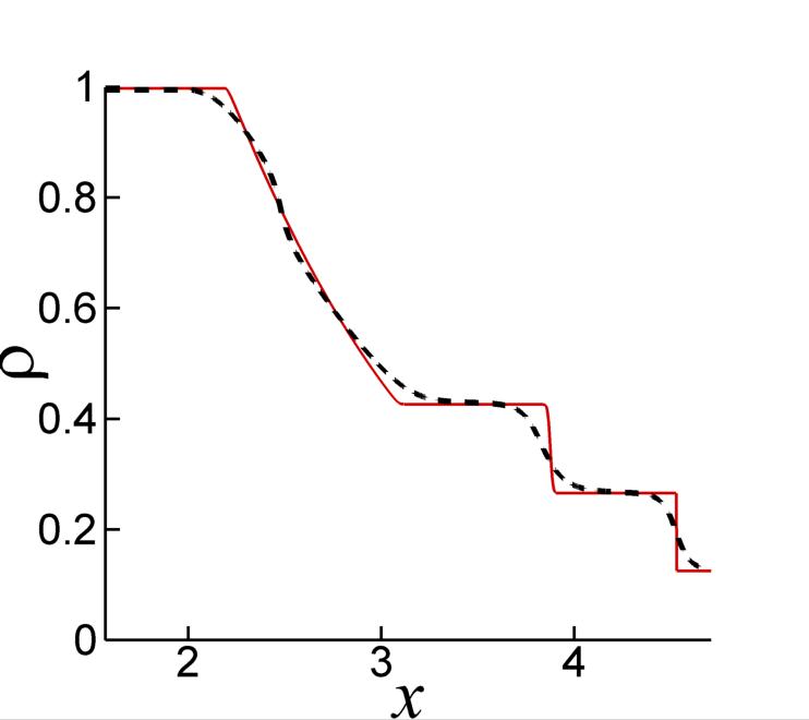
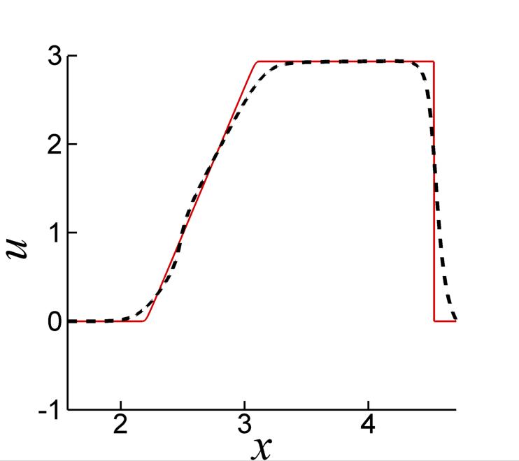
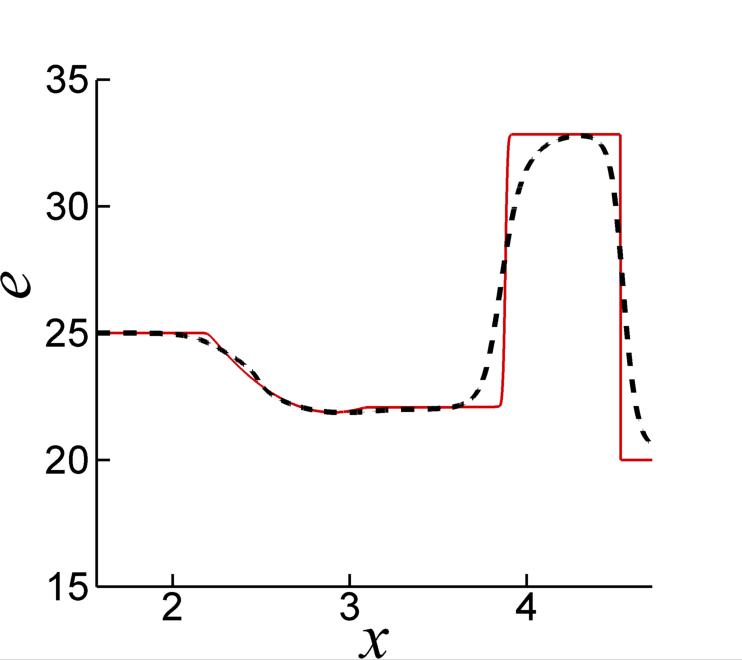
(a)

(b)

(c)

Figure 8: This figure shows a numerical simulation of the regularized Euler equations (dashed line) plotted against the solution to the Euler equations (solid line). Here the value of $\alpha=0.05$ at time $t=0.25$. In the figures, it is clear that the regularized Euler equations are capturing both the expansion wave, contact surface, and shock behavior. (a) The density. (b) The velocity. (c) The energy.

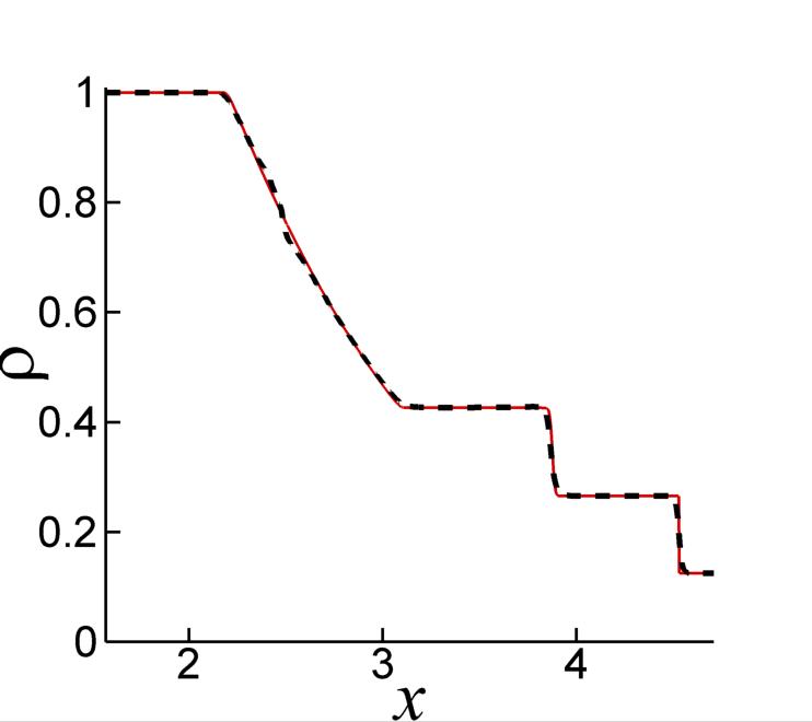
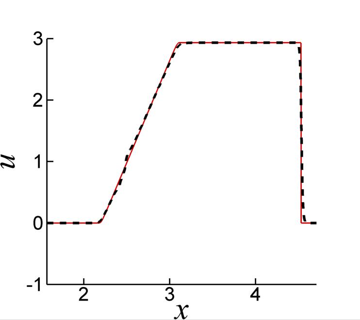
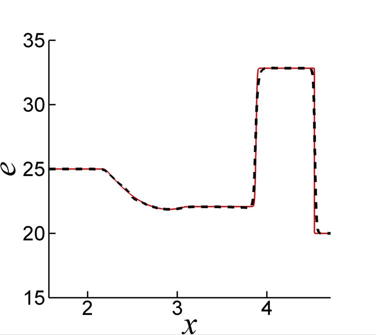
(a)

(b)

(c)

Figure 9: This figure shows a numerical simulation of the regularized Euler equations (dashed line) plotted against the solution to the Euler equations (solid line). Here the value of $\alpha=0.01$ at time $t=0.25$. In the figures, it is clear that the regularized Euler equations are capturing both the expansion wave, contact surface, and shock behavior. With the lower value of $\alpha$ the fit is much closer. (a) The density. (b) The velocity. (c) The energy.

As before we check the convergence of the solutions of the regularized Euler equations to the solution of the Euler equations as $\alpha\to 0$. Figures 10, 11, and 12 show that as $\alpha\to 0$ the error in the $L^{1}$ norm appears to be approaching zero for the example problem. This suggests that the solutions of the regularized Euler equations converge to the solutions of the Euler equations.

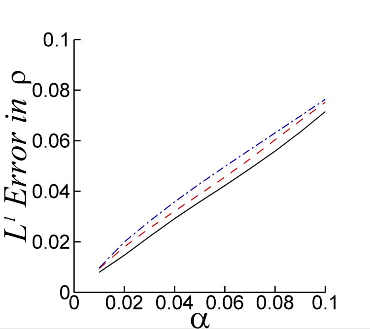
Figure 10: This figure displays the difference between the density in solutions of the regularized Euler equations and the solution of the Euler equations in the $L^{1}$ norm as $\alpha\to 0$. As $\alpha\to 0$ the difference in the solutions also approaches zero. The measurements were taken for $\alpha=0.01,0.02,...,0.1$ at times $t=0.05$,   , $t=0.15$                , and $t=0.25$                        .

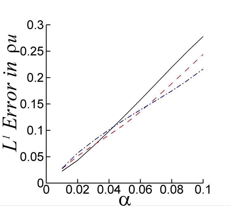
Figure 11: This figure displays the difference between the momentum in solutions of the regularized Euler equations and the solution of the Euler equations in the $L^{1}$ norm as $\alpha\to 0$. As $\alpha\to 0$ the difference in the solutions also approaches zero. The measurements were taken for $\alpha=0.01,0.02,...,0.1$ at times $t=0.05$,   , $t=0.15$                , and $t=0.25$                        .

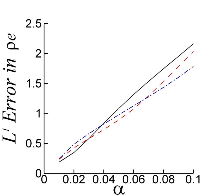
Figure 12: This figure displays the difference between the energy in solutions of the regularized Euler equations and the solution of the Euler equations in the $L^{1}$ norm as $\alpha\to 0$. As $\alpha\to 0$ the difference in the solutions also approaches zero. The measurements were taken for $\alpha=0.01,0.02,...,0.1$ at times $t=0.05$,   , $t=0.15$                , and $t=0.25$                        .

7.7 Kinetic energy rates

As in section 6.8, we examine the kinetic energy for the shock tube problem. Again for the shock tube problem, the solution to the Euler equations are self similar, depending only on the variable $\frac{x}{t}$ and thus the kinetic energy changes linearly in time. For the Euler equations, we examine the kinetic energy $\frac{1}{2}\rho u^{2}$ and for the regularized Euler equations we examine an unfiltered kinetic energy $\frac{1}{2}\rho u^{2}$ and a filtered kinetic energy $\frac{1}{2}\bar{\rho}\bar{u}^{2}.$ Other filtered kinetic energies were also considered, but as in the homentropic case, for this example problem, the differences between them and $\frac{1}{2}\bar{\rho}\bar{u}^{2}$ were negligible.

Figure 13 shows how the kinetic energies for the regularized Euler equations behave for various values of $\alpha.$ Again after a brief period, the energies seem to vary linearly with time. We attribute this brief period to the averaging of the initial conditions. As $\alpha$ decreases the energies for the regularized Euler equations approach the energy of the Euler equations, as we would expect if the solutions are converging as $\alpha\to 0$.

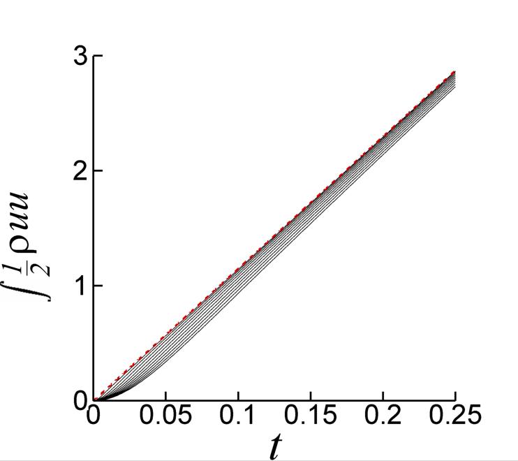
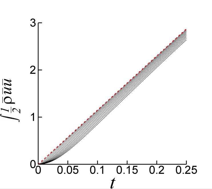
(a)

(b)

Figure 13: The kinetic energy of the Euler equations and the regularized Euler equations. The energy for the true solution of the Euler equations is shown as a dashed red line. The simulation of the regularized Euler equations for $\alpha=0.01,0.02,...,0.1$ are shown as solid black lines. The bottommost line represents $\alpha=0.1$. As $\alpha$ decreases the energy approaches the energy of the Euler equations. (a) These are plots of the unfiltered kinetic energies, $\frac{1}{2}\rho u^{2}$. (b) These are plots of the filtered kinetic energies, $\frac{1}{2}\bar{\rho}\bar{u}^{2}$. When examined the plots of $\frac{1}{2}\overline{\rho u}\bar{u}$ and $\frac{\overline{\rho u}^{2}}{2\bar{\rho}}$ were identical to this one.

8 Conclusion

Using the convectively filtered Burgers (CFB) equations as inspiration we have developed a new averaging technique with the intent of regularizing both shocks and turbulence simultaneously. This paper examines primarily the shocks regularization aspect of the technique. We discussed the physical motivation for the method and then derived a general technique to be used on conservation laws. It was then established that this technique, when applied to conservation laws, would preserve the original conservative properties.

The remainder of the paper then examined the effects when this method was applied to the homentropic Euler and Euler equations. The results show much promise. It was found that with the Helmholtz filter that both the regularized homentropic Euler and regularized Euler equations can be rewritten in conservation form, reiterating that the original conservative properties are preserved. For both sets of equations we were able to find traveling shock solutions, where the Rankine-Hugoniot jump conditions for the modified equations reduced to the same jump conditions of the original equations. For both sets of equations it was proven that as the filtering is decreased, $\alpha\to 0$, the solutions will converge to weak solutions of the original equations. Both these results show that the proper shock speeds of the original equations will be preserved with the averaging techniques.

Numerical simulations were run on both sets of equations for the shock tube problem. These simulations demonstrated that the modified equations mimic the behavior of the original equations. The regularized homentropic Euler equations captured both the expansion wave and the shock front behavior, while the regularized Euler equations captured the expansion wave, contact surface, and the shock front. The solutions appeared regularized meaning that they were continuous and smooth. Furthermore, as $\alpha\to 0$ these solutions were seen to be converging to the solutions of the original equations.

There is still more work to be done regarding these equations. It would be beneficial to establish more theory regarding both sets of equations. Specifically existence proofs would be beneficial. It would be interesting to see if the either sets of equations possess a Hamiltonian structure.

The regularized homentropic Euler and regularized Euler equations are showing promise as a new regularization method based on the preliminary examination considered here. From these results we believe that this averaging technique leads to a regularization of the homentropic Euler and Euler equations that is capable of capturing the relevant behavior of the equations, at least for short time simulations. With future work we hope to establish this more thoroughly and extend this technique into higher dimensions.

9 Acknowledgments

The research in this paper was partially supported by the AFOSR contract FA9550-05-1-0334. We would also like to thanks Dr. Keith Julien for his advice in the numerical simulations.

References

- [1] K. Mohseni, H. Zhao, and J. Marsden. Shock regularization for the Burgers equation. AIAA paper 2006-1516, 44 AIAA Aerospace Sciences Meeting and Exhibit, Reno, Nevada, January 9-12 2006.
- [2] G. Norgard and K. Mohseni. A regularization of the Burgers equation using a filtered convective velocity. J. Phys. A: Math. Theor., 41:1–21, 2008.
- [3] H.S. Bhat and R.C. Fetecau. A Hamiltonian regularization of the Burgers equation. J. Nonlinear Sci., 16(6):615–638, 2006.
- [4] H. S. Bhat and R. C. Fetecau. Stability of fronts for a regularization of the Burgers equation. Quarterly of Applied Mathematics, 66:473–496, 2008.
- [5] G. Norgard and K. Mohseni. On the convergence of convectively filtered Burgers equation to the entropy solution of inviscid Burgers equation. Accepted to SIAM Journal, Multiscale Modeling and Simulation., 2009. Also http://arxiv.org/abs/0805.2176.
- [6] D.D. Holm and M.F. Staley. Wave structures and nonlinear balances in a family of evolutionary PDEs. SIAM J. Appl. Dyn. Syst., 2:323–380, 2003.
- [7] A. Cheskidov, D.D. Holm, E. Olson, and E.S. Titi. On a Leray- model of turbulence. Royal Society London, Proceedings, Series A, Mathematical, Physical & Engineering Sciences, 461(2055):629–649, 2004.
- [8] C. Foias, D. D. Holm, and E. S. Titi. The Navier-Stokes- model of fluid turbulence. Physica D., 152-3:505–519, 2001.
- [9] J.E. Marsden and S. Shkoller. Global well-posedness of the LANS- equations. Proc. Roy. Soc. London, 359:1449–1468, 2001.
- [10] K. Mohseni, B. Kosović, S. Shkoller, and J.E. Marsden. Numerical simulations of the Lagrangian averaged Navier-Stokes (LANS-) equations for homogeneous isotropic turbulence. Phys. Fluids, 15(2):524–544, 2003.
- [11] H. Zhao and K. Mohseni. A dynamic model for the Lagrangian averaged Navier-Stokes- equations. Phys. Fluids, 17(7):075106, 2005.
- [12] D.D. Holm, J.E. Marsden, and T.S. Ratiu. Euler-Poincaré models of ideal fluids with nonlinear dispersion. Phys. Rev. Lett., 349:4173–4177, 1998.
- [13] S.Y. Chen, C. Foias, D.D. Holm, E. Olson, E.S. Titi, and S. Wynne. Camassa-Holm equations as a closure model for turbulent channel and pipe flow. Phys. Rev. Lett., 81:5338–5341, 1998.
- [14] A.A.Ilyin, E.M.Lunasin, and E.S.Titi. A modified Leray- subgrid scale model of turbulence. Nonlinearity, 19:879–897, 2006.
- [15] G. Norgard and K. Mohseni. An examination of the homentropic Euler equations with averaged characteristics. unplublished, 2009. Also http://arxiv.org/abs/0902.4729.
- [16] H. S. Bhat and R. C. Fetecau. Lagrangian averaging for the 1D compressible Euler equations. Discrete and Continuous Dynamical Systems, 6(5):979–1000, 2006.
- [17] H. S. Bhat, R. C. Fetecau, and J. Goodman. A Leray-type regularization for the isentropic Euler equations. Nonlinearity, 20:2035–2046, 2007.
- [18] H. S. Bhat, R. C. Fetecau, J. E. Marsden, K. Mohseni, and M. West. Lagrangian averaging for compressible fluids. SIAM Journal on Multiscale Modeling and Simulation, 3(4):818–837, 2005.
- [19] P. Bradshaw. Turbulence. Springer-Verlag, 1976.
- [20] R.H.Kraichnan. Lagrangian-history statistical theory for Burgers’ equation. The Physics of Fluids, 11(2):265–277, 1968.
- [21] S.N. Gurbatov, S.I. Simdyankin, E. Aurell, U. Frisch, and G. Toth. On the decay of Burgers turbulence. J. Fluid Mech., 344:339–374, 1997.
- [22] C.B. Laney. Computational Gasdynamics. Cambridge University Press, 1998.
- [23] J.K. Hunter and B. Nachtergaele. Applied Analysis. World Scientific, 2001.
- [24] J.Duoandikoetxe. Fourier Analysis. AMS, 2000.
- [25] G.A. Sod. A survey of several finite-differences methods from systems of nonlinear hyperbolic conservation laws. Journal of Computational Physics, 27:1–31, 1978.