Symmetry of Dirac Equation and Corresponding Phenomenology

Abstract

It has been suggested that the high symmetries in the Schrödinger equation with the Coulomb or harmonic oscillator potentials may remain in the corresponding relativistic Dirac equation. If the principle is correct, in the Dirac equation the potential should have a form as ${(1+\beta)\over 2}V(r)$ where $V(r)$ is ${-e^{2}\over r}$ for hydrogen atom and $\kappa r^{2}$ for harmonic oscillator. However, in the case of hydrogen atom, by this combination the spin-orbit coupling term would not exist and it is inconsistent with the observational spectra of hydrogen atom, so that the symmetry of SO(4) must reduce into SU(2). The governing mechanisms QED and QCD which induce potential are vector-like theories, so at the leading order only vector potential exists. However, the higher order effects may cause a scalar fraction. In this work, we show that for QED, the symmetry restoration is very small and some discussions on the symmetry breaking are made. At the end, we briefly discuss the QCD case and indicate that the situation for QCD is much more complicated and interesting.

I introduction

The Schrödinger equation is the basis of non-relativistic quantum mechanics. It successfully explains the energy spectra of hydrogen atom and harmonic oscillator, moreover as the orbit-spin coupling is taken into account, the fine structure of hydrogen atom is also calculated. All the predictions are consistent with measurements of high precision. In a complete theoretical framework which respects the Lorentz covariance, the relativistic Klein-Gorden equation for spin-zero particles and Dirac equation for spin 1/2 particles substitute the Schrödinger equation to describe physics. Surely, under the non-relativistic approximation, they can reduce back to the Schrödinger equation and meanwhile the orbit-spin coupling and relativistic correction terms which were added into the non-relativistic Hamiltonian by hand, automatically appear. Nowadays, as the detection technique and instrumentation are ceaselessly improved, small deviation between theoretical predictions and observational data may be exposed, such as the Lamb shiftLamb ; Lamb2 ; Lamb3 , and it enables one to investigate the tiny difference caused by various theoretical models.

No wonder, as is well known, symmetry is extremely important in all fields of physics. Generally, the Schrödinger equation for hydrogen atom which is of a Coulomb-type potential of N dimensions possesses an SO(N+1) symmetry. It is not a geometric symmetry, but a dynamical one. The SO(4) group in three dimensions can be decomposed into a direct product of two independent SU(2) groups which correspond to spin and orbital angular momenta respectively Greiner . Recently, Zhang, Fu and ChenChen indicate that the Schrödinger equation with a central force fields has an explicit SO(4) symmetry, but generally the Dirac equation with the same potential does not possess the SO(4) symmetry. The harmonic oscillator has the similar situation. The Schrödinger equation has an SU(3) symmetry, but the corresponding Dirac equation does not. GinocchioGinocchio ; Ginocchio2 investigated this problem and obtained a modified Dirac equation which possesses the SU(3) symmetry and can also reduce into the original Schrödinger equation under non-relativistic approximation.

In the central force field the non-relativistic Hamiltonian is $H=\frac{p^{2}}{2m}+V(r)$, turning into the operator form, one only needs to replace ${\bf p}$ into $-i\hbar\nabla$ and does not change the potential $V(r)$ in the configuration representation, the Schrödinger equation of the central force would retain the symmetry of $V(r)$ (${-e^{2}\over r}$ for hydrogen and $\kappa r^{2}$ for harmonic oscillator). By contrast, in the relativistic theory, the Hamiltonian of a free particle should be $H=\sqrt{p^{2}+m^{2}}$, thus if one writes it into an operator form, the square root $\sqrt{p^{2}+m^{2}}$ needs to be replaced by $\mathbf{\alpha}\cdot\mathbf{p}+m\beta$. However, if there was a potential $V(r)$ in the non-relativistic Hamiltonian, then how to write a corresponding term in the Hamiltonian when the Dirac equation replaces the Schrödinger equation, would be a question. In other words, one can ask whether he needs to change its form. The authors of Ref.Chen showed that if we do not make a proper changes on the form of $V(r)$, the corresponding Dirac equation with the central force filed fails to possess the original SO(4) symmetry at all. Alternatively, if we re-write it as $V(r)(1+\beta)/2$, the SO(4) symmetry would be maintained. Generally, The non-relativistic theory is a natural approximation of the relativistic theory, thus one may suppose that the symmetry degree in the relativistic theory should be higher than the non-relativistic one. Therefore, there is a compelling reason to believe that the Dirac equation of hydrogen atom should respect the SO(4) symmetry.

However, the physics does not promise the symmetry argument. As the authors of Ref.Chen indicate, when the Hamiltonian in the Dirac equation is of the form : $\alpha\cdot{\bf p}+\beta M+{1\over 2}(1+\beta)V$, as it reduces into the Schrödinger equation, the spin-orbit coupling term does not exist, namely the $2P_{1/2}$ and $2P_{3/2}$ states should be degenerate, i.e. the fine structure of hydrogen would not be experimentally observed. That conclusion is definitely contrary to the experimental measurement.

Let us investigate the origin of the scalar and vector potentials in the Dirac equations based on the quantum field theory (QFT). Considering all possible Lorentz structures of the interactions which conserve parity, there are five types of interactions between two charged fermions Lucha : $1\otimes 1\sim V_{s}(r)$; $\gamma_{5}\otimes\gamma_{5}\sim 0$; $\gamma^{\mu}\otimes\gamma_{\mu}\sim V_{V}(r)$; $\gamma^{\mu}\gamma_{5}\otimes\gamma_{\mu}\gamma_{5}\sim{\bf S}_{1}\cdot{\bf S}_{2}V_{A}(r)$ and $\sigma_{\mu\nu}\otimes\sigma^{\mu\nu}\sim{\bf S}_{1}\cdot{\bf S}_{2}V_{T}(r)$. As is believed, the underlying theory which is responsible for electromagnetic processes is QED which is a vector-like gauge theory. At the leading order only $\gamma^{\mu}\otimes\gamma_{\mu}$ exists, which induces merely the vector potential $V_{V}(r)$ by exchanging a virtual photon. However, the higher order effects, i.e. multi-photon exchanges can cause scalar and tensor interactions. If we ignore the part $V_{A}(r)$ and $V_{T}(r)$ which are related to the hyper-fine structure in hydrogen atom case and tiny, only the scalar potential should emerge.

The observation raises a serious problem that the high symmetry in the Schrödinger equation which is a non-relativistic approximation of the Dirac equation might be superficial. When the spin-orbit coupling is taken into account, the symmetry would disappear. In other words, in the Schrödinger equation with only the Coulomb’s potential ${-e^{2}\over r}$, the apparent SO(4) symmetry does not survive in the relativistic Dirac equation. Interesting issue is how much the symmetry can be restored. In fact, in some literatures which is aiming to study phenomenology, one writes the potential as $(b+a\beta)V(r)$ with $a+b=1$, and lets $a$ be a free parameter to be fixed by experimental data.

With the form provided in Ref. SVPotential ; SVPotential2 ; SVPotential3 ; SVPotential4 ; SVPotential5 ; SVPotential6 : $H=\alpha\cdot{\bf p}+\beta(M+V_{s})+V_{V}$ and by our above discussion, we write it as $H=\alpha\cdot{\bf p}+\beta M+(b+a\beta)V$, then following Greiner’s calculation which includes all possible combinations of $a$ and $b$, we can use the hydrogen atom spectrum which has been measured with high precision to determine a and b and see to what degree the SO(4) symmetry can be restored or never. We find that for the hydrogen atom, the fraction of the scalar potential is only at order of 0.1%, namely in the QED case (responsible for the hydrogen atom) the symmetry breaking is almost complete, i.e. $SO(4)\longrightarrow SU(2)$.

Based on the quantum field theory, the global and local symmetries which reside in the Lagrangian are real, instead, the symmetries in the Schrödinger equation are indeed superficial. On other aspect, the higher effects can partly restore the symmetry in the potential, in fact, the information can help us understanding the effects of higher orders in QED and even in QCD where higher orders and non-perturbative effects may play a crucial role.

After this long introduction, we will present our numerical results on the hydrogen atom spectrum and determine the fraction of scalar potential in section II. Then we analyze the origin of the scalar potential based on the QED theory and discuss the breakdown of SO(4). The last section is devoted to our conclusion and meanwhile we briefly discuss the QCD case and indicate that for QCD the situation is much more complicated and the symmetry analysis might help us to get a better understanding of the non-perturbative QCD effects and higher order contributions.

II Dirac equation for hydrogen atom

In order to further explore the symmetry problem, we investigate the symmetry issue of the most familiar hydrogen atom which has been thoroughly studied from both theoretical and experimental aspects. In the case of hydrogen atom, the interaction between the electron and proton is purely electromagnetic, so that one can determine to what degree the SO(4) symmetry is broken.

The Dirac equation with an unbroken SO(4) symmetry has the form Chen

$$[c\hat{\alpha}\cdot\hat{p}+mc^{2}\beta+\frac{1+\beta}{2}V(r)-E]\psi=0,$$ (1)

and for hydrogen atom $V(r)=-\frac{e^{2}}{r}$.

In this expression the vector and scalar potentials coexist with the same weight. Its solution is explicitly given in Ref.Greiner ,

$$[c\hat{\alpha}\cdot\hat{p}+\beta(mc^{2}+V_{2})-(E-V_{1})]\psi=0,$$ (2)

where $V_{1}$ and $V_{2}$ are vector and scalar potentials respectively. If one chooses $V_{1}=V_{2}=-\hbar c\frac{\alpha}{2r}=-\frac{e^{2}}{2r},$ he can obtain Eq.1. The spectrum is

$$E=m[1-\frac{2\alpha^{2}}{\alpha^{2}+4n^{2}}],$$ (3)

where the natural unit system $c=\hbar=1$ is adopted and the principal quantum number is $n=n^{\prime}+j+\frac{1}{2}$.

From Eq.(3) we can see that the energy spectrum is determined only by the principal quantum $n$ i.e. the states with various $j-$values are degenerate and there would be no fine-structures, and it is the picture described by the Schrödinger equation whose potential does not involve the spin-orbit couplings.

Generally the Dirac equation for hydrogen atom as only the vector potential being involved, takes the form which is given in ordinary textbooks of quantum mechanics:

$$[c\hat{\alpha}\cdot\hat{p}+mc^{2}\beta-{e^{2}\over r}-E]\psi=0.$$ (4)

The corresponding eigen-energies are

$$E=m[1+\frac{\alpha^{2}}{(s+n^{\prime})^{2}}]^{-\frac{1}{2}},$$ (5)

where $s=\sqrt{(j+\frac{1}{2})^{2}-\alpha^{2}}$ and the energies are explicitly related to quantum number $j$.

We present the eigen-energies corresponding to various $j$ and $l$ when $n=1,2$ in the following table,

Table 1:

$n$	$n^{\prime}$	$j$	$K$	$l$	structure	$E_{1}$(eV)	$E_{2}$(eV)
$1$	0	$\frac{1}{2}$	1	0	$1s_{\frac{1}{2}}$	13.605433412	13.605071149
$2$	0	$\frac{3}{2}$	2	1	$2p_{\frac{3}{2}}$	3.400994390	3.400971749
$2$	1	$\frac{1}{2}$	-1	1	$2p_{\frac{1}{2}}$	3.401039674	3.400971749
$2$	1	$\frac{1}{2}$	1	0	$2s_{\frac{1}{2}}$	3.401039674	3.400971749

where $E_{1}$ and $E_{2}$ are calculated in terms of Eqs.(5) and (3) respectively and the mass of electron and fine-structure constant are set according to Ref. PDG06 . Since the spectrum of hydrogen has been experimentally measured with very high accuracy, we keep more significant figures in our calculation results accordingly. It is shown later that some small distinctions between theory and data only appear at the last few digits of the number.

III Symmetry is restored partly or never

As discussed above, let us rewrite the Dirac equation as

$$[c\hat{\alpha}\cdot\hat{p}+mc^{2}\beta+bV(r)+a\beta V(r)-E]\psi=0,$$ (6)

with $a$ constraint $a+b=1$ which ensures this equation to reduce back to the familiar Schrödinger equation, but now we suppose $a$ and $b$ to be free parameters (in fact, only $a$ or $b$ is free by the constraint).

It is easy to obtain the eigen-energy of hydrogen according to Ref. Greiner as

$$E = m\{\frac{-(1-a)a\alpha^{2}}{(1-a)^{2}\alpha^{2}+(n-j-\frac{1}{2}+s)^{2}}+[(\frac{(1-a)a\alpha^{2}}{(1-a)^{2}\alpha^{2}+(n-j-\frac{1}{2}+s)^{2}})^{2}$$ (7)

$$-\frac{a^{2}\alpha^{2}-(n-j-\frac{1}{2}+s)^{2}}{(1-a)^{2}\alpha^{2}+(n-j-\frac{1}{2}+s)^{2}}]^{\frac{1}{2}}\},$$

Generally, one can determine the parameter $a$ by fitting the data of hydrogen atom. It is noted that all the measured data of hydrogen atoms involve the effects of not only fine structure which results in the splitting of energies corresponding to various j-values, but also the hyper-fine structure and Lamb shift. The hyper-fine structure is due to the interaction between the spins of nucleus (proton in the hydrogen case) and electron, while the Lamb shift is caused by the virtual photon effects. To extract the necessary information about the fine structure, one can either carefully carry out a theoretical estimate to get rid of the influences from other effects or choose special transition modes where only the physical mechanism we concern plays a dominant role. In fact, we may ignore the effects of the hyperfine structure, because it is suppressed by a factor $m_{e}/m_{p}\sim 1/2000$ compared to the fine structure caused by the spin-orbit coupling Landau ; Landau2 .

The energy gap between $2p_{\frac{3}{2}}$ and $2p_{\frac{1}{2}}$ may be a good candidate to study the splitting induced by spin-orbit coupling, since they are in $p$ wave and the Lamb shift is small2pLamb . The level-crossing value between $2p_{\frac{3}{2}}$ and $2p_{\frac{1}{2}}$ has been measured as $10969.20\pm 0.06$MHz2p2p . Using this value we obtain $a=-(8.93\pm 0.02)\times 10^{-4}$ ( $a/b=-0.000893$) which manifests the restoration degree of the SO(4) symmetry.

There are three comments,

(1) Since $a$ is a very small number, Eq.(6)is very close to Eq.(4), i.e. the symmetry breaking in the QED case is almost complete.

(2) Especially, $a$ is negative. Since this value is obtained by fitting data, we should suppose that it is valid. Question is what the negative sign implies? As we discuss above, the SO(4) symmetry demands $a=b=1/2$, if $a$ were a small positive value, we could allege that the SO(4) symmetry were partly restored, but now it is a small negative value, what conclusion can we draw? We will come to this question at the last section.

(3) Even though there is a scalar potential in Eq.(6), the mechanisms which induce the Lamb shift and hyper-fine-structure are not involved in the Dirac equation (Eq.(6)) as aforementioned.

Table 2:

$n$	$n^{\prime}$	$j$	$K$	$l$	spectrum	eigen-values (eV)
$1$	0	$\frac{1}{2}$	1	0	$1s_{\frac{1}{2}}$	13.605434057
$2$	0	$\frac{3}{2}$	2	1	$2p_{\frac{3}{2}}$	3.400994431
$2$	1	$\frac{1}{2}$	-1	1	$2p_{\frac{1}{2}}$	3.401039795
$2$	1	$\frac{1}{2}$	1	0	$2s_{\frac{1}{2}}$	3.401039795

IV Origin of scalar potential in quantum field theory

In principle, we can make a general discussion about how the scalar potential emerges in the relativistic quantum mechanics. The least action principle in quantum mechanics tells us how to construct the Hamiltonian for a charged particle in electromagnetic field by transforming operator ${\bf p}$ into ${\bf p}-e{\bf A}$ and $E$ into $E-e\phi(r)$ where $\phi(r)$ is the zeroth component of $A^{\mu}$. The corresponding Dirac equation would be of the form $[\mathbf{\alpha}\cdot\mathbf{p}+m\beta+\phi(r)]\psi=E\psi$ where only the vector potential exists, because the energy $E$ has the same Lorentz structure as $\phi$ and it is exactly $V_{V}(r)$ we concern. If the non-relativistic Hamilton can be written as $H=\sqrt{p^{2}+(m+V(r))^{2}}$, after the transformation, we can obtain a different equation $[\mathbf{\alpha}\cdot\mathbf{p}+(m+V(r))\beta]\psi=E\psi$, because now the potential $V$ has the same Lorentz structure as the mass and then $V$ is a scalar potential. However there is no reason to write the Hamiltonian in that way.

Now let us turn to the QED theory which is viewed as the correct theory to be responsible for all the electromagnetic processes, at the quantum field theory level. As aforementioned, the QED is a vector coupling theory, so that at the leading order the scalar potential does not exist. One can ask if the scalar potential emerges at higher orders. The answer is positive: actually we can deduce a scalar coupling from high order QED. Due to the fundamental coupling between electron and photon $\overline{\psi}_{e}\gamma_{\mu}\psi_{e}A^{\mu}$, we achieve the vector potential from a single photon exchangeGreiner ; Zuber .

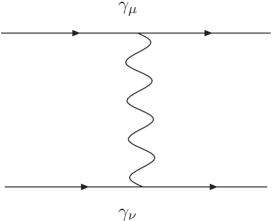
Figure 1:

When the high order effects are taken into account, namely, as we consider the loop contributions, the scalar coupling appears. The next to leading order Feynman diagrams with two photons exchanged between electrons are shown in Fig.2 and 3. Omitting irrelevant factors in the amplitude, we can write it as

$$M\propto\int\bar{U}(P_{b})\gamma_{\rho}\frac{P_{1}\!\!/+m_{1}}{P_{1}^{2}-m_{1}^{2}}\gamma_{\mu}U(P_{a}){d^{4}P_{1}\over(2\pi)^{4}}\bar{U}(P_{d})\gamma_{\omega}\frac{P_{2}\!\!\!/+m_{2}}{P_{2}^{2}-m_{2}^{2}}\gamma_{\nu}U(P_{c})g^{\rho\omega}g^{\mu\nu}\frac{1}{(P_{a}-P_{1})^{2}(P_{1}-P_{b})^{2}}.$$ (8)

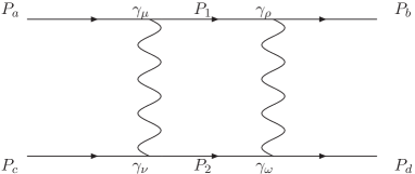
Figure 2:

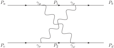
Figure 3:

The term

$$\bar{U}(P_{b})\gamma_{\rho}\frac{-m_{1}}{P_{1}^{2}-m_{1}^{2}}\gamma_{\mu}U(P_{a})\bar{U}(P_{d})\gamma_{\omega}\frac{-m_{2}}{P_{2}^{2}-m_{2}^{2}}\gamma_{\nu}U(P_{c})g^{\rho\omega}g^{\mu\nu}\frac{1}{(P_{a}-P_{1})^{2}(P_{1}-P_{b})^{2}},$$ (9)

can be rewritten as

$$\frac{m_{1}m_{2}}{(P_{1}^{2}-m_{1}^{2})(P_{2}^{2}-m_{2}^{2})}\bar{U}(P_{b})\gamma_{\rho}\gamma_{\mu}U(P_{a})\bar{U}(P_{d})\gamma_{\omega}\gamma_{\nu}U(P_{c})g^{\rho\omega}g^{\mu\nu}\frac{1}{(P_{a}-P_{1})^{2}(P_{1}-P_{b})^{2}}.$$ (10)

A simple relation

$$\gamma_{\alpha}\gamma_{\beta}=\frac{1}{2}(\gamma_{\alpha}\gamma_{\beta}-\gamma_{\beta}\gamma_{\alpha})+\frac{1}{2}(\gamma_{\alpha}\gamma_{\beta}+\gamma_{\beta}\gamma_{\alpha})=g_{\alpha\beta}-i\sigma_{\alpha\beta},$$ (11)

leads to

$$\frac{m_{1}m_{2}}{(P_{1}^{2}-m_{1}^{2})(P_{2}^{2}-m_{2}^{2})}\bar{U}(P_{b})g_{\rho\mu}U(P_{a})\bar{U}(P_{d})g_{\omega\nu}U(P_{c})g^{\rho\omega}g^{\mu\nu}$$

$$=\frac{m_{1}m_{2}}{(P_{1}^{2}+m_{1}^{2})(P_{2}^{2}+m_{2}^{2})}\bar{U}(P_{b})U(P_{a})\bar{U}(P_{d})U(P_{c})\frac{1}{(P_{a}-P_{1})^{2}(P_{1}-P_{b})^{2}},$$ (12)

which is explicitly a $1\times 1$ type coupling and eventually induces a scalar potential. The Feynman diagram in Fig.3 also results in similar scalar coupling.

Now let us turn to study the form of the induced potential. In fact, the integration is complicated and usually cannot be analytically derived. This is similar to deriving a potential between two nucleons induced by two-pion exchange. Instead of making a full integration over $q$ which is supposed to correspond to the one-loop radiative correction to the scattering amplitude, we would like to derive the main piece of an effective potential between two charged particles. Let us focus on the two photon propagators in Eq.(IV), we write the term as

$${1\over q^{2}(q+P)^{2}},$$ (13)

where $q=P_{1}-P_{b}$ and $P=P_{b}-P_{a}$, and the two fermion propagators are quenched.

The standard wayLandau ; Landau2 of obtaining a potential in QFT is to carry out a Fourier transformation on ${\bf P}$ in the transition amplitude. Now let us see the integration

$$I = \int\frac{dq^{4}}{(2\pi)^{4}}\int{e^{i{\bf P}\cdot{\bf r}}\over q^{2}[(q_{0}+P_{0})^{2}-(\mathbf{q}+\mathbf{P})^{2}]}d^{3}\mathbf{P},$$ (14)

$$= \int\frac{dq^{4}}{(2\pi)^{4}}\int{e^{i{\bf P}\cdot{\bf r}}\over q^{2}[q_{0}^{2}-(\mathbf{q}+\mathbf{P})^{2}]}d^{3}\mathbf{P},$$

where the loop integration over four-momentum $q$ can be carried out in the regular way. For the Fourier integration, following the standard, we set $P_{0}=0$. Shifting the integration variable ${\bf P}$ into $\bf P^{\prime}=P+q$, we have

$$I = \int\frac{dq^{4}}{(2\pi)^{4}}\int{e^{i({\bf P^{\prime}-q})\cdot{\bf r}}\over q^{2}[q_{0}^{2}-\bf P^{\prime 2}]}d^{3}\mathbf{P^{\prime}}$$ (15)

$$= \int\frac{dq^{4}}{(2\pi)^{4}}{e^{-i{\bf q}\cdot{\bf r}}\over q^{2}}\int{e^{i({\bf P^{\prime}})\cdot{\bf r}}\over[q_{0}^{2}-\bf P^{\prime 2}]}d^{3}\mathbf{P^{\prime}}.$$

The contour integration is standard and one immediately obtains the results in terms of the residue principle as

$$I = \int\frac{dq^{4}}{(2\pi)^{4}}{e^{-i{\bf q}\cdot{\bf r}}\over q^{2}}\frac{e^{-|q_{0}||\bf r|}}{\mathbf{r}}$$ (16)

$$= \frac{1}{\mathbf{r}}\int\frac{dq^{4}}{(2\pi)^{4}}{e^{-i{\bf q}\cdot{\bf r}}\over q^{2}}e^{-|q_{0}||\bf r|}.$$

It shows that the leading term in the induced potential is a generalized Coulomb-type, even though the numerator in Eq.(16) is not a simple rational number, but an integration. It is worth noting that the numerator in Eq.(16) corresponds to the loop integration which is not Lorentz invariant because we have already chosen the rest frame of the the two-fermion system as our reference frame. To really calculate it, one may need to deal with possible infrared divergence which appears for soft photon propagation, but anyhow, it is a number. It is beyond the scope of this work, here we only show the characteristic of the potential induced by the two-photon exchange. Indeed, such a potential induced by the two-photon exchange is very complicated and it is in analog to the interaction between nucleons induced by two-pion exchange which has been thoroughly studied by many authorsChemtob . The potential form is not easy to be framed, generally can be better described by the Bethe-Salpeter equation Rocha . In Ref. Rocha , the authors gave a very complicated potential form, but one can notice that the leading piece is still the Yukawa-type one which corresponds to the Coulomb-type in the case of two photon-exchange.

As carrying out above theoretical calculations, we only consider the scalar Coulomb type potential in Eq.(11), but definitely when fitting data, contributions from all other pieces are involved altogether. It seems that our theoretical calculation is not complete. However, the contributions from other pieces are either of the same order of magnitude or, most probably, smaller than the contributions of the Coulomb piece. Therefore, as we discuss the symmetry breaking and restoration in this work, we only concern the order of magnitude, thus our results which only involve contribution from the Coulomb piece do make sense. In other words, our derivation is not rigorous, but is illustrative and persuasive. We will carry out a complete derivation of the two-photon induced potential in our later work. It also interesting to note that the sign of the Coulomb-type potential induced by two-photon exchange is opposite to that induced by one-photon exchange. It can naturally explain the minus sign of $a$ obtained by fitting data.

Because the scaler coupling arise at the next to leading order so the scalar potential should generally undergo a loop suppression. By a simple analysis of order of magnitude, this suppression factor is proportional to $\alpha/\pi=\frac{1}{137\pi}\simeq 0.00232$ relative to the vector potential. Definitely the concrete suppression factor should be derived by explicitly calculating the loop diagrams and numerically evaluate the contributions. But as the order $O(\alpha^{2})$ and even higher orders can contribute to the scalar potential, we would like to obtain the suppression factor $a/b$ phenomenologically. The number on $a/b$ which is obtained by fitting the spectrum of hydrogen and the value was given in last section, one can notice that it is consistent with our qualitative analysis.

V Conclusion and discussion

It is a well-known fact that symmetry plays an important role in physics. Not only the geometric symmetries are obviously important, but also dynamical symmetries are fundamental and crucial for determining the physics. For example, It has been a long time, people notice that there is an extra symmetry $[{\bf R},H]=0$ with ${\bf R}={1\over 2m}({\bf p}\times{\bf L}-{\bf L}\times{\bf p})-{e^{2}\over r}\mathbf{\hat{r}}$ for the hydrogen atom. This symmetry finally leads to the $n^{2}$ degeneracy of the hydrogen levels Baym . The symmetry corresponds to two “angular momenta” and the generators are respectively

$${\bf M}={{\bf L}+{\bf K}\over 2};$$

and

$${\bf N}={{\bf L}-{\bf K}\over 2},$$

where ${\bf K}\equiv\sqrt{{-m\over 2H}}{\bf R}$. The two “angular momenta” symmetries are involved in a larger group SO(4).

Similarly, it is indicated that the Hamiltonian of harmonic oscillator has an SU(3) dynamical symmetry. Since the Schrödinger equation is the relativistic approximation of the relativistic Dirac equation for fermions, one can ask if the larger symmetries are maintained in the corresponding Dirac equations? The symmetry causes degeneracy and the symmetry breaking leads to splitting of energy levels, thus to answer the question, we need to study the observational energy level splitting. Ginocchio Ginocchio ; Ginocchio2 and Zhang et al. Chen indicate that to maintain the higher symmetry in the Dirac equations for harmonic oscillator and hydrogen atom, the scalar and vector potentials must have the same weight, i.e. the combination is of the form $(1+\beta)V(r)$. If one changes the combination into $(a+b\beta)V(r)$ with $a+b=1$, as he reduces the Dirac equation into the non-relativistic Schrödinger equation, at the leading order, the combination does not induce distinction because $\beta=\left(\begin{array}[]{cc}I&0\\ 0&-I\end{array}\right)$, only the left corner entry plays a role. But to the next order, the right corner entry joins the game and $a$ and $b$ terms would have different contributions and the superficial symmetry is broken unless $a=b=1/2$. If so, the spin-orbit coupling does not exist and fine structure (energy splitting) disappears. It obviously contradicts to the experimental observation.

The underlying theory is QED which is a vector-like theory, and its leading order contribution to the potential is via the one-photon exchange which definitely results in a vector potential in the Dirac equation. Even though the higher order QED effects would induce the scalar potential, it should be much suppressed comparing to the leading term. The data tell us that the fraction of the scalar potential is at order of 0.1% which is consistent with our estimation based on the quantum field theory. We obtain the value of $a$ as $a=-(8.93\pm 0.02)$ ( $a/b=-0.00089$) by fitting the hydrogen spectrum, and it seems that the value further deviates from $a=b=1/2$ which is demanded by the SO(4) symmetry. Does the negative sign really mean that the symmetry is not partly restored? Since the value of $a$ is too small, some theoretical and experimental uncertainties can cause a small fluctuation in the value, so that we cannot yet draw a definite conclusion that the symmetry is not restored. To confirm its sign, one must pursue this study in a case where the restoration might be sizable, and no doubt it is the QCD case.

Since the higher order contributions of QCD would be much more important because $\alpha_{s}$ is large at lower energies, so one can expect that in the QCD case, such symmetry restoration might be significant. Castro and FranklinFranklin ; Franklin2 ; Franklin3 ; Franklin4 have worked out the Dirac equation where the authors considered an arbitrary combination of the scalar and vector potentials for both the Coulomb and linear pieces and obtain the wavefunction of ground state of a $q\bar{q}$ bound state. Interesting aspect is that they find that the dominant part in the linear confinement potential is the scalar part. That conclusion is obviously different from the QED case. Since the linear potential is fully due to the long-distance effects of QCD and may be caused by the non-perturbative contributions, we cannot derive it from QFT so far (in the the lattice theory, the area theorem may imply a linear potential form, but cannot distinguish the vector and scalar fractions at all.), the argument about the origin of scalar potential given in last section becomes incomplete. We will further pursue this interesting issue and it is the goal of our next workKe .

Our conclusion is whether the high symmetries in the Schrödiner equation may exist in the corresponding Dirac equation needs careful studies. In the case of hydrogen atom, it definitely does not. We show that the symmetry breaking is almost complete, from the experimental and theoretical aspects.

Indeed it would an interesting problem because we explicitly show the breaking for hydrogen atom, but for other kinds of potentials which may be induced by various mechanisms, especially the phenomenological potentials such as the Cornell-type potential which is responsible for the quark confinement, whether such symmetry can be kept in the Dirac equation is worth further investigation.

References

- (1) W. Lamb, Jr. and R. Retherford, Phys. Rev. 72 , 241 (1947).
- (2) W. Lamb, Jr. and R. Retherford, Phys. Rev. 75 , 1325 (1949).
- (3) W. Lamb, Jr. and R. Retherford, Phys. Rev. 79 , 549 (1950).
- (4) W. Greiner, Relativistic Quantum Mechanics, Springer, Berlin(2000).
- (5) F. Zhang, B. Fu and J. Chen, Phys. Rev. A 78 , 040101(R) (2008).
- (6) J. Ginocchio, Phys. Rev. C 69 , 034318 (2004).
- (7) J. Ginocchio, Phys. Rev. Lett. 95, 252501(2005).
- (8) W. Lucha, F. Schöberl and D. Gromes, Phys. Rep. 200 (1991) 127.
- (9) J. N. Ginocchio, Phys. Rep. 414, 165 (2005).
- (10) A. Leviatan, Phys. Rev. Lett. 92, 202501 (2004).
- (11) A. L. Blokhin, C. Bahri, and J. P. Draayer, Phys. Rev. Lett. 74, 4149 (1995).
- (12) S.-G. Zhou, J. Meng, and P. Ring, Phys. Rev. Lett. 91, 262501 (2003).
- (13) K. Sugawara-Tanabe and A. Arima, Phys. Rev. C 58, R3065 1998.
- (14) P. Page, T. Goldman and J. Ginocchio, Phys. Rev. Lett. 86, 204 (2001).
- (15) W. Yao ., Partical Data Group, J. Phys. G 33, 1 (2006).
- (16) V. Berestetskii, E. Lifshitz and L. Pitaevskii, Quantum Eletrodynamics, Pergamon Press Ltd. (1982).
- (17) Landshoff and Nachtmann, Zeit. f. Physik C35, 405(1988).
- (18) R. Beausoleil, D. McIntyre, C. Foot, E. Hildum, B. Couilaud and T. Hänsch, Phys. Rev. A 35 , 4878 (1987).
- (19) S. Kaufman, W. Lamb, Jr., K. Lea and M. Leventhal, Phys. Rev. Lett. 22 , 507 (1969).
- (20) C. Itzykson and J. Zuber, Quantum Field Theory, McGraw-Hill(1980).
- (21) M. Chentob, J. Durso and D. Riska, Nucl. Phys. B38 (1972) 141;
- (22) C. Rocha and M. Robilotta, Phys.Rev. C49 (1994) 1818.
- (23) G. Baym, Lectures on Quantum Mechanics, The Benjamin/Cummings Pub. Com. Inc, (1969).
- (24) J. Franklin, Mod. Phys. Lett. A14, 2409 (1999).
- (25) A. d. Castro and J. Franklin, hep-ph/0011137 .
- (26) A. d. Castro and J. Franklin, Int. Mod. Phys. A15, 4355 (2000).
- (27) H. Crater, J. Yoon, and C. Wong, Phy. Rev. D79, 034011 (2009).
- (28) H. Ke and X. Li, in preparation.