Single-photon entanglement concentration for long-distance quantum communication

Abstract

We present a single-photon entanglement concentration protocol for long-distance quantum communication with quantum nondemolition detector. It is the first concentration protocol for single-photon entangled states and it dose not require the two parties of quantum communication to know the accurate information about the coefficient $\alpha$ and $\beta$ of the less entangled states. Also, it does not resort to sophisticated single-photon detectors, which makes this protocol more feasible in current experiments. Moreover, it can be iterated to get a higher efficiency and yield. All these advantages maybe make this protocol have more practical applications in long-distance quantum communication and quantum internet.

I introduction

Quantum entanglement is a unique phenomenon and its distribution over a long distance is of vital importance in quantum information. Many quantum processes require entanglement book ; rmp ; densecoding ; teleportation . The simplest entanglement may be a single-photon entanglement with the form $\frac{1}{\sqrt{2}}(|1\rangle_{A}|0\rangle_{B}+|0\rangle_{A}|1\rangle_{B})=\frac{1}{\sqrt{2}}(a^{\dagger}+b^{\dagger})|0\rangle$. It is a superposition state in location A or B. Here, $|0\rangle$ and $|1\rangle$ represent the photon number 0 and 1, respectively. Currently, the most important application for single-photon entanglement may be the quantum repeater protocol in long-distance quantum communication repeater1 ; repeater2 ; repeater3 . For instance, in Duan-Lukin-Cirac-Zoller (DLCZ) quantum communication scheme repeater1 , with one pair source and one quantum memory at each location, the quantum repeater is to entangle two remote locations A and B. The pair sources are coherently excited by synchronized classical pumping pulses, and then they emit a pair with a small probability $p/2$, corresponding to the state

$$[1+\sqrt{\frac{p}{2}}(a^{\dagger}a^{\prime\dagger}+b^{\dagger}b^{\prime\dagger})+o(p)]|0\rangle.$$ (1)

Here, $a^{+}$ ($b^{+}$, $a^{\prime+}$ or $b^{\prime+}$) is the creation operation for the mode $a$ ($b$, $a^{\prime}$ or $b^{\prime}$). The two parties of quantum communication, say the sender Alice and the receiver Bob, store the modes $a$ and $b$ in their quantum memories in locations A and B, respectively, and send $a^{\prime}$ and $b^{\prime}$ to a station located in the middle of A and B, where they are combined by a 50:50 beam splitter (BS). One can create the single-photon entangled state $\frac{1}{\sqrt{2}}(a^{\dagger}+b^{\dagger})|0\rangle$ between two distant locations A and B by detecting the photon after the BS. Furthermore, this entangled state can be converted into a two-atom entangled state with the form $\frac{1}{\sqrt{2}}(|e\rangle_{A}|g\rangle_{B}+|g\rangle_{A}|e\rangle_{B})$ atom ; cabrillo ; chou1 ; chou2 . Here $|e\rangle$ is the excited state and $|g\rangle$ is the grounded state of a two-level atom. In this way, we can extend the entanglement to two long-distance locations by using entanglement swapping to complete the task of long-distance quantum communication repeater1 .

In a practical quantum repeater, Alice and Bob cannot ensure that their entangled states are maximal ones. That is, they cannot ensure the pair sources excited by the synchronized classical pumping pulses always have the same probability, which means they usually obtain some pure entangled states, instead of maximally entangled ones. Meanwhile, in a practical transmission, an entangled quantum system inevitably interacts with its environment, which will degrade its entanglement with another form. For example, a maximally entangled state may become a mixed entangled one, which may make a long-distance quantum communication infeasible. The way of distilling a set of mixed entangled states into a subset of maximally entangled states is named as entanglement purification Bennett1 ; Deutsch ; Pan1 ; Simon ; shengpra1 . Another method of distilling a set of less entangled pure states into a subset of maximally entangled states, which will be detailed here, is named as entanglement concentration. In 1996, Bennett et al. proposed an entanglement concentration protocol which is called Schmidt projection method Bennett2 . Another similar protocol is called entanglement swapping swapping1 ; swapping2 . But the entanglement swapping protocol fails to concentrate single-photon entanglement here. In 2001, Yamamoto et al. Yamamoto and Zhao et al. zhao1 independently proposed two similar two-photon entanglement concentration protocols based on linear optical elements. In 2008, an efficient two-photon entanglement concentration protocol based on cross-Kerr nonlinearity shengpra2 was presented. In these three two-photon entanglement concentration protocols Yamamoto ; zhao1 ; shengpra2 , it is unnecessary for Alice and Bob to know the coefficients of the less entangled states accurately.

Although there are some good entanglement purification Bennett1 ; Deutsch ; Pan1 ; Simon ; shengpra1 and entanglement concentration schemes Bennett2 ; swapping1 ; swapping2 ; Yamamoto ; zhao1 ; shengpra2 , they all focus on the polarization entanglement states for photon pairs, not single-photon entanglements. Fortunately, Sangouard et al. proposed the first single-photon entanglement purification protocol singlepurification with linear optics in 2008. It is used to purify the phase error. It is rather simple and feasible with current technology, but it is an important progress for the implementation of quantum repeater protocols for long-distance quantum communication. In this paper, we will propose an entanglement concentration protocol for single-photon entanglement with quantum nondemolition detectors based on cross-Kerr nonlinearity. It is the first entanglement concentration protocol for single-photon entangled states $(\alpha a^{+}+\beta b^{+})|0\rangle$ and it dose not require the two parties to know the accurate information about the coefficient $\alpha$ and $\beta$ of the less entangled pure states. Also, it does not resort to sophisticated single-photon detectors, which makes this protocol more feasible in current experiments. Moreover, this protocol can be iterated to get a higher efficiency and yield than the conventional entanglement concentration protocols. This single-photon entanglement concentration protocol and the entanglement purification protocol in Ref.singlepurification may constitute important progresses for the implementation of the quantum repeater protocols based on single-photon entanglement in long-distance quantum communication repeater1 and quantum internet.

II The problem of entanglement concentration for long-distance quantum communication

In a practical manipulation, we cannot ensure the pair sources excited by the synchronized classical pumping pulses always have the same probability. We still take DLCZ scheme repeater1 as an example to describe the principle. The pair source in location A is coherently excited and can emit a pair with the following form:

$$|0\rangle_{a}|0\rangle_{a^{\prime}}+\sqrt{\frac{p_{a}}{2}}a^{\dagger}a^{\prime\dagger}|0\rangle_{a}|0\rangle_{a^{\prime}}+o(p_{a}),$$ (2)

but in location B, the pair source may emit a pair with the form:

$$|0\rangle_{b}|0\rangle_{b^{\prime}}+\sqrt{\frac{p_{b}}{2}}b^{\dagger}b^{\prime\dagger}|0\rangle_{b}|0\rangle_{b^{\prime}}+o(p_{b}).$$ (3)

$\frac{p_{a}}{2}$ and $\frac{p_{b}}{2}$ are two different probabilities for locations A and B, respectively. In this time, the whole system evolves as:

$$[1+\sqrt{\frac{p_{a}}{2}}a^{\dagger}a^{\prime\dagger}|0\rangle_{a}|0\rangle_{a^{\prime}}+\sqrt{\frac{p_{b}}{2}}b^{\dagger}b^{\prime\dagger}|0\rangle_{b}|0\rangle_{b^{\prime}}+o(p)]|0\rangle.$$ (4)

Finally, after the detection of the photon combined by a BS, the single-photon entangled state becomes $(\sqrt{\frac{p_{a}}{2}}a^{\dagger}+\sqrt{\frac{p_{b}}{2}}e^{i\theta_{AB}}b^{\dagger})|0\rangle$. We can rewrite it as:

$$|\Psi^{\prime}\rangle_{ab}=(\alpha a^{\dagger}+\beta e^{i\theta_{AB}}b^{\dagger})|0\rangle,$$ (5)

where $|\alpha|^{2}+|\beta|^{2}=1$. $\theta_{AB}$ is the relative phase between A and B. This relative phase is sensitive to the path length instabilities between two remote entangled pairs, and it will make the long-distance quantum communication difficult repeater0 ; repeater . Eq.(5) is the entanglement of photonic modes, and we can convert it to the memory modes with $M_{A}$ and $M_{B}$. The memory modes will let the two memories be in the excited state or in the ground state. Meanwhile, the quantum memory systems can also lead to the same phenomena with different probabilities for the photons storing in A and B as they both interact with their environments.

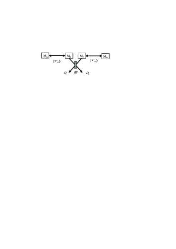
Figure 1: The setup of entanglement connection in the DLCZ protocol repeater1 . BS is a 50:50 beam splitter. After this swapping, if one of the detectors registers one photon, the entanglement between $M_{A}$ and $M_{D}$ can be set up.

After the entanglement generation, we need to extend the entanglement to long distance with entanglement swapping for long-distance quantum communication. See from Fig.1, if the entangled state of $M_{A}$ and $M_{B}$ and that of $M_{C}$ and $M_{D}$ are both the maximally entangled ones, we can easily establish the maximal entanglement between $M_{A}$ and $M_{D}$ repeater1 . However, if we cannot get the maximally entangled states during the stage of entanglement generation, or the environment noises degrade the maximally entangled states to the form of Eq.(5), the combination of $|\Psi^{\prime}\rangle_{ab}$ and $|\Psi^{\prime}\rangle_{cd}$ can be written as:

$$|\Psi^{\prime}\rangle_{ab}\otimes|\Psi^{\prime}\rangle_{cd}$$

$$=(\alpha a^{\dagger}+\beta e^{i\theta_{AB}}b^{\dagger})\otimes(\alpha c^{\dagger}+\beta e^{i\theta_{CD}}d^{\dagger})|0\rangle$$

$$=(\alpha^{2}a^{\dagger}c^{\dagger}+\beta^{2}e^{i(\theta_{AB}+\theta_{CD})}b^{\dagger}d^{\dagger})|0\rangle$$

$$+(\alpha\beta e^{i\theta_{AB}}b^{\dagger}c^{\dagger}+\alpha\beta e^{i\theta_{CD}}a^{\dagger}d^{\dagger})|0\rangle.$$ (6)

Here we let $|\Psi^{\prime}\rangle_{cd}$ have the same form as $|\Psi^{\prime}\rangle_{ab}$, i.e., $|\Psi^{\prime}\rangle_{cd}=(\alpha c^{\dagger}+\beta e^{i\theta_{CD}}d^{\dagger})|0\rangle$. The BS will makes $b^{\dagger}|0\rangle\rightarrow\frac{1}{\sqrt{2}}(D^{\dagger}_{1}+D^{\dagger}_{2})|0\rangle$ and $c^{\dagger}|0\rangle\rightarrow\frac{1}{\sqrt{2}}(D^{\dagger}_{1}-D^{\dagger}_{2})|0\rangle$. After the 50:50 BS, from Eq.(6) we find that if one of the detectors clicks one photon, we get

$$|\Psi^{\prime\prime}\rangle_{ad}=(\alpha^{2}a^{\dagger}\pm\beta^{2}d^{\dagger}e^{i(\theta_{AB}+\theta_{CD})})|0\rangle.$$ (7)

The ’+’ or ’-’ depends on the click of the detector $D_{1}$ or $D_{2}$. Compared with Eq.(5), the entanglement of Eq.(7) is degraded after the entanglement connection. This problem can be generalized to a more general case. For instance, we perform entanglement swapping protocol for $n$ times to connect the entanglement between the remote locations A and K, we will get

$$|\Psi^{n+1}\rangle_{ak}=(\alpha^{n+1}a^{\dagger}\pm\beta^{n+1}k^{\dagger}e^{i\theta_{AK}})|0\rangle.$$ (8)

For $\alpha\neq\beta$, the entanglement decreases more and more, and we will fail to establish a perfect long-distance entanglement channel for quantum communication. In other words, a long-distance quantum communication with a practical manipulation of entanglement generation and a practical transmission requires the entanglement concentration of single-photon entangled states.

III entanglement concentration of single-photon entanglements

Cross-Kerr nonlinearity has been wildly studied QND1 ; QND2 ; discriminator ; qubit1 ; qubit2 ; qubit3 , such as the construction of a CNOT gate, the discrimination of unknown qubits, Bell-state analysis, and so on. The Hamiltonian of the cross-Kerr nonlinearity is $H_{ck}=\hbar\chi a^{+}_{s}a_{s}a^{+}_{p}a_{p}$ QND1 ; QND2 ; kerr1 ; kerr2 , where $a^{+}_{s}$ and $a^{+}_{p}$ are the creation operations and $a_{s}$ and $a_{p}$ are the destruction operations. When the coherent beam $|\alpha\rangle_{p}$ and a signal pulse in the Fock state $|\Psi\rangle_{s}=c_{0}|0\rangle_{s}+c_{1}|1\rangle_{s}$ interact with the cross-Kerr nonlinearity, the whole system becomes:

$$U_{ck}|\Psi\rangle_{s}|\alpha\rangle_{p} = e^{iH_{ck}t/\hbar}[c_{0}|0\rangle_{s}+c_{1}|1\rangle_{s}]|\alpha\rangle_{p}$$ (9)

$$= c_{0}|0\rangle_{s}|\alpha\rangle_{p}+c_{1}|1\rangle_{s}|\alpha e^{i\theta}\rangle_{p},$$

where $\theta=\chi t$ and $t$ is the interaction time. One can see that the phase shift of the coherent beam is proportional to the number of photons in the Fock state. We can use this good feature to construct a quantum nondemolition detector (QND).

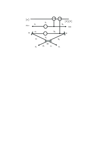
Figure 2: The principle of our single-photon entanglement concentration protocol. Alice and Bob share two single-photon entangled states with the form $\frac{1}{\sqrt{2}}(a^{\dagger}+b^{\dagger})|0\rangle$. A 50:50 beam splitter (BS) is located in the middle of A and B, and it is used to couple the two modes $a_{2}$ and $b_{2}$. Homodyne detector of the QND is used to distinguish the photon number. After the detection of $D_{1}$ and $D_{2}$, the two parties can get some maximally entangled states with the probability $2|\alpha\beta|^{2}$.

The principle of our single-photon entanglement concentration protocol is shown in Fig.2. Alice and Bob want to share the maximally entangled state $|\Psi\rangle_{ab}=\frac{1}{\sqrt{2}}(a^{\dagger}+b^{\dagger})|0\rangle$. We suppose that there are two identical less entangled states $|\Psi\rangle_{a_{1}b_{1}}$ and $|\Psi\rangle_{a_{2}b_{2}}$ shared by Alice and Bob. One is in the mode ${a_{1}b_{1}}$ and the other is in the mode ${a_{2}b_{2}}$. The two single-photon less entangled sates are

$$|\Psi\rangle_{a_{1}b_{1}} = (\alpha a^{\dagger}_{1}+\beta e^{i\theta_{A_{1}B_{1}}}b^{\dagger}_{1})|0\rangle,$$ (10)

$$|\Psi\rangle_{a_{2}b_{2}} = (\alpha a^{\dagger}_{2}+\beta e^{i\theta_{A_{2}B_{2}}}b^{\dagger}_{2})|0\rangle.$$ (11)

In this protocol, we suppose the two sources emit the entangled state simultaneously, so the path length fluctuations of two channels $a_{1}b_{1}$ and $a_{2}b_{2}$ can be regarded as the same one, then the phase $\theta_{A_{1}B_{1}}$ equals to $\theta_{A_{2}B_{2}}$. We give them a general sign as $\theta_{AB}$. The original state of these two photons can be rewritten as

$$|\Phi\rangle = |\Psi\rangle_{a_{1}b_{1}}\otimes|\Psi\rangle_{a_{2}b_{2}}$$ (12)

$$= (\alpha^{2}a^{\dagger}_{1}a^{\dagger}_{2}+\alpha\beta e^{i\theta_{AB}}a^{\dagger}_{1}b^{\dagger}_{2}$$

$$+ \alpha\beta e^{i\theta_{AB}}a^{\dagger}_{2}b^{\dagger}_{1}+\beta^{2}e^{2i\theta_{AB}}b^{\dagger}_{1}b^{\dagger}_{2})|0\rangle.$$

$a^{\dagger}_{1}a^{\dagger}_{2}$ and $b^{\dagger}_{1}b^{\dagger}_{2}$ represent that the two photons both belong to Alice and Bob, respectively. $a^{\dagger}_{1}b^{\dagger}_{2}$ and $a^{\dagger}_{2}b^{\dagger}_{1}$ mean that each of Alice and Bob owns a photon. One can see that $a^{\dagger}_{1}b^{\dagger}_{2}$ and $a^{\dagger}_{2}b^{\dagger}_{1}$ have the same coefficient $\alpha\beta e^{i\theta_{AB}}$, and the other two terms have the different coefficients. Now Bob lets the two modes $b_{1}$ and $b_{2}$ enter a QND. With a homodyne measurement $|X\rangle\langle X|$, Bob may get three different results: $a^{\dagger}_{1}a^{\dagger}_{2}$ leads no phase shift on the coherent beam, $b^{\dagger}_{1}b^{\dagger}_{2}$ leads to the phase shift $2\theta$, and $a^{\dagger}_{1}b^{\dagger}_{2}$ and $a^{\dagger}_{2}b^{\dagger}_{1}$ lead to the phase shift $\theta$. So if the phase shift of the homodyne measurement is $\theta$, Bob requires Alice to keep this result; otherwise both of them discard this measurement. In this way, if we omit the global phase factor $e^{i\theta_{AB}}$, the state of the remaining quantum system becomes

$$|\Phi\rangle^{\prime}=\frac{1}{\sqrt{2}}(a^{\dagger}_{1}b^{\dagger}_{2}+a^{\dagger}_{2}b^{\dagger}_{1})|0\rangle.$$ (13)

The probability that Alice and Bob get the state $|\Phi\rangle^{\prime}$ is $2|\alpha\beta|^{2}$.

The modes $a_{2}$ and $b_{2}$ are reflected and coupled by a 50:50 BS which will make

$$a^{\dagger}_{2}|0\rangle \rightarrow \frac{1}{\sqrt{2}}(c^{\dagger}_{2}-d^{\dagger}_{2})|0\rangle,$$ (14)

$$b^{\dagger}_{2}|0\rangle \rightarrow \frac{1}{\sqrt{2}}(c^{\dagger}_{2}+d^{\dagger}_{2})|0\rangle.$$ (15)

That is, Eq.(13) evolves as

$$|\Phi\rangle^{\prime} \rightarrow \frac{1}{2}[a^{\dagger}_{1}(c^{\dagger}_{2}+d^{\dagger}_{2})+b^{\dagger}_{1}(c^{\dagger}_{2}-d^{\dagger}_{2})]|0\rangle$$ (16)

$$= \frac{1}{2}[(a^{\dagger}_{1}+b^{\dagger}_{1})c^{\dagger}_{2}+(a^{\dagger}_{1}-b^{\dagger}_{1})d^{\dagger}_{2}]|0\rangle.$$

One can see that if the detector $D_{1}$ fires, the state of the remaining quantum system is left to be

$$|\Phi_{1}\rangle^{\prime}=\frac{1}{\sqrt{2}}(a^{\dagger}_{1}+b^{\dagger}_{1})|0\rangle;$$ (17)

otherwise, the detector $D_{2}$ fires and the quantum system collapses to

$$|\Phi_{2}\rangle^{\prime}=\frac{1}{\sqrt{2}}(a^{\dagger}_{1}-b^{\dagger}_{1})|0\rangle.$$ (18)

They both are maximally single-photon entangled states. There is a phase difference between Eq.(18) and Eq.(17). In polarization entanglement concentration protocol, one can easily perform a phase-flipping operation to correct this analogous phase error Bennett2 ; swapping1 ; swapping2 ; Yamamoto ; zhao1 ; shengpra2 . However, for a single-photon entanglement, a phase-flipping operation is not easily performed. Certainly, we can convert Eq.(18) into Eq.(17) with the help of quantum memory repeater1 .

With only one QND, the probability that Alice and Bob get the state $|\Phi\rangle^{\prime}$ shown in Eq.(13) is $2|\alpha\beta|^{2}$. This protocol does not require Alice and Bob to know the accurate information about the coefficients $\alpha$ and $\beta$ of the less entangled pure states. In fact, this probability is not the maximal one. In the above protocol, Alice and Bob only pick up the instances that the phase shift is $\theta$ and discard the other cases. If a suitable cross-Kerr material can be provided, or the interaction time can be controlled accurately, Alice and Bob will get the phase shift $\theta=\pi$ when one photon is detected. In this time, if two photons pass through the QND, they will make the phase shift with $2\theta=2\pi$. $2\pi$ is the same phase shift as 0. In this case, Eq.(12) collapses to

$$|\Phi\rangle^{\prime\prime}=(\alpha^{2}a^{\dagger}_{1}a^{\dagger}_{2}+\beta^{2}e^{2i\theta_{AB}}b^{\dagger}_{1}b^{\dagger}_{2})|0\rangle.$$ (19)

This state is not a maximally entangled one, but with the next step one can also get the maximally one with single-photon entanglement concentration. After coupled by the BS, Eq.(19) becomes

$$|\Phi\rangle^{\prime\prime} = [\frac{\alpha^{2}}{\sqrt{2}}a^{\dagger}_{1}(c^{\dagger}_{2}-d^{\dagger}_{2})+\frac{\beta^{2}e^{2i\theta_{AB}}}{\sqrt{2}}b^{\dagger}_{1}(c^{\dagger}_{2}+d^{\dagger}_{2})]|0\rangle$$ (20)

$$= [(\frac{\alpha^{2}}{\sqrt{2}}a^{\dagger}_{1}-\frac{\beta^{2}e^{2i\theta_{AB}}}{\sqrt{2}}b^{\dagger}_{1})c^{\dagger}_{2}$$

$$+ (\frac{\alpha^{2}}{\sqrt{2}}a^{\dagger}_{1}+\frac{\beta^{2}e^{2i\theta_{AB}}}{\sqrt{2}}b^{\dagger}_{1})d^{\dagger}_{2}]|0\rangle.$$

If the detector $D_{1}$ fires, the state in Eq.(20) is transformed into

$$|\Phi_{1}\rangle^{\prime\prime}=(\alpha^{2}a^{\dagger}_{1}-\beta^{2}e^{2i\theta_{AB}}b^{\dagger}_{1})|0\rangle.$$ (21)

If the detector $D_{2}$ fires, it is transformed into

$$|\Phi_{2}\rangle^{\prime\prime}=(\alpha^{2}a^{\dagger}_{1}+\beta^{2}e^{2i\theta_{AB}}b^{\dagger}_{1})|0\rangle.$$ (22)

It is easy to find that Eq.(22) has the same form as Eq.(5). So does the second less entangled state in Eq.(21). The whole system becomes

$$|\Phi\rangle^{\prime\prime\prime} = |\Phi_{2}\rangle^{\prime\prime}_{a_{1}b_{1}}\otimes|\Phi_{2}\rangle^{\prime\prime}_{a_{2}b_{2}}$$ (23)

$$= (\alpha^{4}a^{\dagger}_{1}a^{\dagger}_{2}+\alpha^{2}\beta^{2}e^{i2\theta_{AB}}a^{\dagger}_{1}b^{\dagger}_{2}$$

$$+ \alpha^{2}\beta^{2}e^{i2\theta_{AB}}a^{\dagger}_{2}b^{\dagger}_{1}+\beta^{4}e^{i4\theta_{AB}}b^{\dagger}_{1}b^{\dagger}_{2})|0\rangle.$$

Following the method above and the help of QND, Alice and Bob pick up $a^{\dagger}_{1}b^{\dagger}_{2}$ and $a^{\dagger}_{2}b^{\dagger}_{1}$ with the probability of $2|\alpha^{2}\beta^{2}|^{2}$, and they keep the other terms for next iteration. Eq.(21) can also be manipulated with the same step as that discussed above. Finally, one can perform this protocol by iteration of the process above and get a higher yield of maximally entangled states.

IV discussion and conclusion

In our protocol, only one QND is used to detect the photon number in spatial modes. If the modes $a_{1}a_{2}$ and $b_{1}b_{2}$ both contain one photon, the phase shift of the coherent beam is $\theta$, which can be easily detected by a homodyne measurement. Different from single-photon entanglement purification protocol singlepurification , this protocol does not require sophisticated single-photon detectors as the QND has the function of a photon number detector.

Let us compare this single-photon entanglement concentration protocol with the conventional two-photon entanglement concentration protocols proposed in Refs.Yamamoto ; zhao1 ; shengpra2 . In fact, all of these four protocols are based on the principle of Schmidt projection method, but the conventional protocols are focused on polarization entanglement states of two-photon quantum systems, not Fock states of single-photon quantum systems. The polarization beam splitter zhao1 and the QND shengpra2 act as the same role of parity check. Here the QND acts as the role of a photon-number detector for two spatial modes, but does not destroy the Fock states of the two spatial modes. This role can not simply be replaced with a photon-number detector as a photon-number detection on the spatial modes $b_{1}$ and $b_{2}$ will change their Fock states and make entanglement concentration fail. Another difference is that this protocol requires nonlocal operations. In Refs.Yamamoto ; zhao1 ; shengpra2 , after the parity check, Alice and Bob both perform Hadamard operations on the remaining photons and detect them locally. However, this single-photon entanglement concentration protocol works for neighbor nodes in a long-distance quantum communication. Alice and Bob need to combine the modes $a_{2}$ and $b_{2}$ into the beam splitter in the middle location of A and B if the phase shift picks up $\theta$. This combination principle is similar to the creation of single-photon entanglement in DLCZ protocol repeater1 . In principle, this single-photon entanglement concentration protocol has the efficiency $Y$,

$$Y = \sum_{i=1}^{n}Y_{i},$$ (24)

where

$$Y_{1} = |\alpha\beta|^{2},$$

$$Y_{2} = \frac{1}{2}(1-2|\alpha\beta|^{2})\frac{|\alpha\beta|^{4}}{(|\alpha|^{4}+|\beta|^{4})^{2}},$$

$$Y_{3} = \frac{1}{2^{2}}(1-2|\alpha\beta|^{2})[1-\frac{|\alpha\beta|^{4}}{(|\alpha|^{4}+|\beta|^{4})^{2}}]\frac{|\alpha\beta|^{8}}{(|\alpha|^{8}+|\beta|^{8})^{2}},$$

$$\;\;\;\;\;\;\;\;\;\;\;\;\;\;\;\;\ldots$$

$$Y_{n} = \frac{1}{2^{n-1}}(1-2|\alpha\beta|^{2})\left(\prod^{n-1}_{j=3}[1-\frac{2|\alpha\beta|^{2^{j-1}}}{(|\alpha|^{2^{j-1}}+|\beta|^{2^{j-1}})^{2}}]\right)$$ (25)

$$\frac{|\alpha\beta|^{2^{n}}}{(|\alpha|^{2^{n}}+|\beta|^{2^{n}})^{2}}.$$

This efficiency is the same as that in two-photon entanglement concentration with QND shengpra2 , higher than that with PBSs and photon-number detections Yamamoto ; zhao1 as the efficiency in the latter is $Y_{1}$.

Finally, we briefly discuss the problem of relative phase instability in DLCZ protocol repeater1 , which makes the original DLCZ protocol extremely difficult. The relative phase between two remote entangled states is caused by the path length fluctuation, and it must be kept stabilized until the entangled channel is established repeater ; repeater0 . It exists both in the entanglement generation stage and the entanglement connection stage. Here we propose an entanglement concentration protocol during the entanglement transformation. We suppose that the two sources emit the entangled states simultaneously. Therefor, the path length fluctuation of $a_{1}b_{1}$ and $a_{2}b_{2}$ should be the same one. After performing this single-photon entanglement concentration protocol, the relative phase between two copies of entangled states is automatically eliminated, and the single-photon entangled state kept becomes the standard maximally entangled one. The phase also does not appear in the next entanglement connection stage.

In conclusion, we have proposed a scheme for single-photon entanglement concentration, which is realizable with current technology. This protocol has several advantages. First, it does not require the two parties of quantum communication to know accurately the coefficients $\alpha$ and $\beta$ of the single-photon less entangled pure states $(\alpha a^{+}+\beta b^{+})|0\rangle$. This advantage makes this protocol capable of concentrating an arbitrary less entangled pure state. Second, it does not require sophisticated single-photon detectors to judge the photon number in each side. Moreover, this protocol can be iterated to get a higher efficiency and yield than the ordinary concentration protocols. This single-photon entanglement concentration protocol and the entanglement purification protocol in Ref.singlepurification may constitute important progresses for the implementation of the quantum repeater protocols based on single-photon entanglement. Furthermore, these two protocols may provide practical applications in long-distance quantum communication and the construction of the quantum internet internet in future.

References

- (1) M. A. Nielsen and I. L. Chuang, Quantum Computation and Quantum Information (Cambridge University Press, Cambridge, UK, 2000).
- (2) N. Gisin, G. Ribordy, W. Tittel, and H. Zbinden, Rev. Mod. Phys. 74, 145 (2002).
- (3) C. H. Bennett and S. J. Wiesner, Phys. Rev. Lett. 69, 2881 (1992).
- (4) C. H. Bennett, G. Brassard, C. Crepeau, R. Jozsa, A. Peres, and W. K. Wootters, Phys. Rev. Lett. 70, 1895 (1993).
- (5) L. M. Duan, M. D. Lukin, J. I. Cirac, and P. Zoller, Nature 414, 22 (2001).
- (6) C. Simon, H. de Riedmatten, M. Afzelius, N. Sangouard, H. Zbinden, and N. Gisin, Phys. Rev. Lett. 98, 190503 (2007).
- (7) N. Sangouard, C. Simon, J. Minar, H.Zbinden, H. deRiedmatten, and N. Gisin, Phys. Rev. A 76, 050301(R) (2007).
- (8) S. J. van Enk, Phys. Rev. A 72, 064306 (2005).
- (9) C. W. Chou, J. Laurat, H. Deng, K. S. Choi, H. de Reidmatten, D. Felinto, and H. J. Kimble, Science 316, 1316 (2007).
- (10) C. W. Chou, H. de Riedmatten, D. Felinto, S. V. Polyakov, S. J. van Enk, and H. J. Kimble, Nature (London) 438, 828 (2005).
- (11) C. Cabrillo, J. I. Cirac, P. García-Fernàndez, and P. Zoller, Phys. Rev. A 59, 1025 (1999).
- (12) C. H. Bennett, G. Brassard, S. Popescu, B. Schumacher, J. A. Smolin and W. K. Wootters, Phys. Rev. Lett. 76, 722 (1996).
- (13) D. Deutsch, A. Ekert, R. Jozsa, C. Macchiavello, S. Popescu and A. Sanpera, Phys. Rev. Lett 77, 2818 (1996).
- (14) J. W. Pan, C. Simon, and A. Zellinger, Nature (London) 410, 1067 (2001).
- (15) C. Simon and J. W. Pan, Phys. Rev. Lett. 89, 257901 (2002).
- (16) Y. B. Sheng, F. G. Deng, and H. Y. Zhou, Phys. Rev. A 77, 042308 (2008).
- (17) C. H. Bennett, H. J. Bernstein, S. Popescu, and B. Schumacher, Phys. Rev. A 53, 2046 (1996).
- (18) S. Bose, V. Vedral, and P. L. Knight, Phys. Rev A 60, 194 (1999).
- (19) B. S. Shi, Y. K. Jiang, and G. C. Guo, Phys. Rev. A 62, 054301 (2000).
- (20) T. Yamamoto, M. Koashi, and N. Imoto, Phys. Rev. A 64, 012304 (2001).
- (21) Z. Zhao, J. W. Pan, and M. S. Zhan, Phys. Rev. A 64, 014301 (2001).
- (22) Y. B. Sheng, F. G. Deng, and H. Y. Zhou, Phys. Rev. A 77, 062325 (2008).
- (23) N. Sangouard, C. Simon, T. Coudreau, and N. Gisin, Phys. Rev. A 78, 050301(R) (2008).
- (24) B. Zhao, Z. B. Chen, Y. A. Chen, J. schmiedmayer, and J. W. Pan, Phys. Rev. Lett. 98, 240502(2007).
- (25) Z. B. Chen, B. Zhao, Y. A. Chen, J. schmiedmayer, and J. W. Pan, Phys. Rev. A 76, 022329(2007).
- (26) K. Nemoto and W. J. Munro, Phys. Rev. Lett. 93, 250502 (2004).
- (27) S. D. Barrett, P. Kok, K. Nemoto, R. G. Beausoleil, W. J. Munro, and T. P. Spiller, Phys. Rev. A 71, 060302(R) (2005).
- (28) K. Pieter, W. J. Munro, K. Nemoto, T. C. Ralph, J. P. Dowling, and G. J. Milburn, Rev. Mod. Phys. 79, 135 (2007).
- (29) H. F. Hofmann, K. Kojima, S. Takeuchi, and K. Sasaki, J. Opt. B: Quantum Semiclassical Opt. 5, 218 (2003).
- (30) B. He, J. A. Bergou, and Y. H. Ren, Phys. Rev. A 76, 032301 (2007).
- (31) Y. M. Li, K. S. Zhang, and K. C. Peng, Phys. Rev. A 77, 015802 (2008).
- (32) H. Jeong and N. B. An, Phys. Rev. A 74, 022104 (2006).
- (33) G. S. Jin, Y. Lin, and B. Wu, Phys. Rev. A 75, 054302 (2007).
- (34) H. J. Kimble, Nature (London) 453, 1023 (2008).