Robust ecological pattern formation induced by demographic noise

Abstract

We demonstrate that demographic noise can induce persistent spatial pattern formation and temporal oscillations in the Levin-Segel predator-prey model for plankton-herbivore population dynamics. Although the model exhibits a Turing instability in mean field theory, demographic noise greatly enlarges the region of parameter space where pattern formation occurs. To distinguish between patterns generated by fluctuations and those present at the mean field level in real ecosystems, we calculate the power spectrum in the noise-driven case and predict the presence of fat tails not present in the mean field case. These results may account for the prevalence of large-scale ecological patterns, beyond that expected from traditional non-stochastic approaches.

Many years ago, Turing showed how diffusion, normally thought of as a homogenizing influence, can give rise to pattern-forming instabilitiesTuring (1953). Only recently, however, have field observations provided strong support for the presence of Turing patterns in ecosystems, where diffusional processes abound, at least in principle. The slow moving tussock moth population in California together with its faster moving parasites Maron and Harrison (1997) as well as several plant-resource systems Reitkerk and van de Koppel (2008) have been identified as satisfying, qualitatively at least, the key requirements for diffusion driven pattern formation. Observed patterns of plankton populations have also been proposed to arise from Turing instabilities, at least over short length scales Levin and Segel (1976); Malchow et al. (1998); Davis et al. (1992); Abraham (1998).

The common feature of these systems is positive feedback coupled to slow diffusion (usually associated with a species labeled an “activator” that activates both itself and another species called the “inhibitor”), and negative feedback coupled to faster diffusion associated with the inhibitor. This combination of diffusion and feedback promotes the formation of patterns, because local patches are promoted through positive feedback, but are only able to spread a limited distance before the fast diffusion and associated negative feedback of the inhibitor prevents further spread. It is hypothesized that this mechanism is responsible for a great deal of ecosystem level pattern formation Reitkerk and van de Koppel (2008); Maron and Harrison (1997).

One particular class of ecological pattern forming systems, predator-prey (or organism-natural enemy) systems has been extensively analyzed theoretically (see for example, Levin and Segel (1976); Mimura and Murray (1978); Baurmann et al. (2007); Malchow et al. (1998); Mobilia et al. (2006)) and is beginning to allow qualitative comparison to field data along with more system specific theory Maron and Harrison (1997); Wilson et al. (1999). A difficulty in directly comparing the results of this large body of theory to field observations is that in many cases, models only exhibit Turing instabilities if the predator diffusivity is much larger than the prey diffusivity or the parameters are fine tuned Levin and Segel (1976); Mimura and Murray (1978); Wilson et al. (1999); Baurmann et al. (2007). The qualitative argument made above for pattern formation does not depend on very large differences in diffusivities, nor on additional ecological details, and indeed, there are ecological pattern-forming systems which do not apparently display very large separation of diffusivities Maron and Harrison (1997); Reitkerk and van de Koppel (2008). So what is the origin of pattern formation in such systems?

One approach to such questions of ordering is to include levels of detail that in some sense force the response of the system. For example, whereas simple mean field predator-prey models do not show population oscillations, they can be made to do so by the inclusion of predator satiation effectsMaynard Smith (1974). However, such levels of realism do not need to be invoked, because there is a simpler explanation: intrinsic or demographic noise. This may seem counterintuitive, because adding noise to a system is usually thought of as reducing ordering by adding entropy; and indeed, this is exactly what is observed in several models, such as percolation models of epidemics Davis et al. (2008) and spin models of forest canopy gaps Katori et al. (1998). Surprisingly, however, systematic treatments of individual-level models (ILMs) of predator-prey dynamics show that the population fluctuations become amplifiedMcKane and Newman (2005), and lead to time-dependent oscillations (quasi-cycles) that can be distinguished from deterministic limit cycle behaviorPineda-Krch et al. (2007). Disappointingly, to date, no novel spatial effects of demographic noise have been identified, despite several attemptsLugo and McKane (2008); Butler and Reynolds (2009).

In this Rapid Communication, we demonstrate that noise-induced pattern formation arises in a simple but biologically-relevant predator-prey model, and show that if it is analyzed as an ILM, patterns occur over a much larger range of ecologically relevant parameters than predicted by MFT, even in the thermodynamic limit. We accomplish this by calculating the phase diagram and power spectrum of the model analytically. We also predict that experimental noise driven patterns will have power spectra with fat tails not present in patterns driven by instabilities present in MFT. Finally, we show that quasi-cycles are also present, and we provide an interpretation of the spatiotemporal dynamics that result.

I Heuristic analysis of the Levin-Segel model

Among the simplest models of ecological pattern formation was originally introduced to model plankton-herbivore dynamicsLevin and Segel (1976). This model takes the form

$$\begin{split}\partial_{t}\psi&=\mu\nabla^{2}\psi+b_{1}\psi+e\psi^{2}-(p_{1}+p_{2})\psi\varphi\\ \partial_{t}\varphi&=\nu\nabla^{2}\varphi+p_{2}\varphi\psi-d\varphi^{2}\end{split}$$ (1)

where the plankton population density is given by $\psi$, the herbivore population density is given by $\varphi$, $b_{1}$ is birthrate for the plankton, $p_{1}$ and $p_{2}$ are predation, $d$ is competition-driven death of the predators and $e$ corresponds to a community effect, that is the prey facilitates its own birth rate. In the original presentation of this model, this term was intended to be a proxy for reduced predator efficiency at higher prey concentrations Levin and Segel (1976). It can also be interpreted as an Allee effect, wherein many species have enhanced reproduction at higher concentrations (for a review, see Courchamp et al. (1999)). From here on, we set $p_{1}=0$ and $p_{2}=p$ for transparency of analysis. This does not change the qualitative results. The parameters $e$ and $p,\ d$ identify the prey as the activator and the predator as the inhibitor in the mechanism for pattern formation above and distinguish this model from the standard Lotka-Volterra based individual level models recently analyzed and demonstrated not to contain patterns in Lugo and McKane (2008); Butler and Reynolds (2009).

The model contains a stable homogeneous coexistence state when

$$\begin{split}p>e\ \text{and}\ p^{2}>de\end{split}$$ (2)

with fixed point populations given by

$$\psi=\frac{b_{1}d}{p^{2}-de},\ \ \varphi=\frac{b_{1}p}{p^{2}-de}$$ (3)

It contains a Turing instability if Levin and Segel (1976)

$$\frac{\nu}{\mu}>\left(\frac{1}{\left(\sqrt{p/d}-\sqrt{p/d-e/p}\right)}\right)^{2}$$ (4)

When the model violates the stability conditions in Eq. 2, the plankton population diverges and a plankton regulation term (i.e. $-f\psi^{3}$) is required to make the model valid. Such a term would only materially affect the outcomes of this analysis near the instability, where it would decrease the set of parameters for which pattern formation occurs. To examine the behavior of the model, we take the generic set of $O(1)$ kinetic parameters $b_{1}=1/2,\ e=1/2,\ d=1/2$ and $p=1$. With these generic parameters Eq. 4 shows that non-generic diffusivities, $\nu/\mu>27.8$, are required for pattern formation. Similar results are obtained for other stable, generic parameter sets.

Demographic noise may change this pictureWilson (1998) by inhibiting the decay of transient patterns. Turing instabilities occur when, for some specific set of wave vectors, small perturbations no longer decay. However, we expect that even when the parameters are tuned away from the Turing instability, perturbations with some wavelengths may decay more slowly than others, leading to transient patterns. Demographic noise would maintain these patterns by generating continual perturbations. This is reminiscent of extrinsic noise driven patterns reported in other contexts García-Ojalvo et al. (1993); Carrillo et al. (2004); Sieber et al. (2007).

To quantify this heuristic argument, we look at the Fourier transformed dynamics of the fluctuations from the coexistence fixed point with added white noise $\xi$, variance 1. These dynamics are given by

$$-i\omega\bf{x}=\bf{A}\bf{x}+\xi$$ (5)

The matrix $\bf{A}$ is the Fourier transformed stability matrix

$$\bf{A}=\left(\begin{array}[]{cc}-\nu k^{2}-p\psi&p\varphi\\ -p\psi&-\mu k^{2}+e\psi\end{array}\right)$$ (6)

Simple manipulations yield the power spectrum

$$\begin{split}&P(k,\omega)=\left[p^{2}\varphi^{2}+(e\psi-\mu k^{2})^{2}\right]\times\bigg{[}\big{(}pb_{1}\psi+\mu\nu k^{4}-\omega^{2}\\ &-\psi k^{2}e\nu\left(1-\frac{p\mu}{e\nu}\right)\big{)}^{2}+\omega^{2}((e-p)\psi-(\mu+\nu)k^{2})\bigg{]}^{-2}\end{split}$$ (7)

Very approximately, we expect from Eq. 7 that patterns (indicated by peaks in the power spectrum) form whenever $e\nu>p\mu$. This is much less stringent than Eq. 4 and can be satisfied for generic sets of parameters. However, to reliably demonstrate our hypotheses and extract experimental predictions, we next perform a systematic study of demographic noise from an individual level model.

II Individual Level Model

We define the individual level version of the model by considering a locally well mixed patch of volume $V$. We consider the following reactions

$$P \stackrel{{\scriptstyle b_{1}}}{{\rightarrow}}PP\ \ PP \stackrel{{\scriptstyle e/V}}{{\rightarrow}}PPP$$

$$PH \stackrel{{\scriptstyle p/V}}{{\rightarrow}}HH\ \ HH \stackrel{{\scriptstyle d/V}}{{\rightarrow}}H$$ (8)

where $P$ denotes plankton and $H$ denotes herbivores, with the parameters as described above. Stochastic trajectories of $H$ and $P$, enumerated by $m$ and $n$ respectively, are described by the master equation

$$\partial_{t}P(m,n)=b_{1}(-nP(m,n)+(n-1)P(m,n-1))$$

$$+\frac{e}{V}[(n-1)(n-2)P(m,n-1)-n(n-1)P(m,n)]$$

$$+\frac{p}{V}(-mnP(m,n)+(m-1)(n+1)P(m-1,n+1))$$

$$+\frac{d}{V}\left[(m+1)mP(m+1,n)-m(m-1)P(m,n)\right]$$ (9)

To analyze the master equation, we map it to a path integral formulation of bosonic field theory and generalize to space Doi (1976); Goldenfeld (1984); Mikhailov (1981); Peliti (1985); Janssen and Tauber (2005). To add space we consider a lattice of patches, and random hopping for both species at different rates between nearest neighbor patches. The resulting Lagrangian density is given by

$$\mathcal{L}= \hat{x}\partial_{t}z+\hat{\rho}\partial_{t}\rho-\nu\hat{z}\nabla^{2}z-\mu\hat{\rho}\nabla^{2}\rho-\nu z(\nabla\hat{z})^{2}$$

$$-\mu\rho(\nabla\hat{\rho})^{2}+b_{1}\rho(1-e^{\hat{\rho}})+\frac{e}{V}\rho^{2}(1-e^{\hat{\rho}})$$

$$+\frac{p}{V}z\rho(1-e^{\hat{z}-\hat{\rho}})+\frac{d}{V}z^{2}(1-e^{-\hat{z}})$$ (10)

Where $\hat{z},\;z$ are noise and number variables respectively for herbivores, and similarly, $\hat{\rho},\;\rho$ are noise and number variables for plankton. To analyze this Lagrangian directly is difficult, due to exponential terms and diffusive noise. To make progress, we derive a systematic expansion and mean field theory (MFT) in powers of $\sqrt{V}$ motivated by the $\Omega$-expansion Van Kampen (1992); Butler and Reynolds (2009). We assume the forms

$$\hat{z} \rightarrow\frac{\hat{z}}{\sqrt{V}} \hat{\rho} \rightarrow\frac{\hat{\rho}}{\sqrt{V}}$$ (11)

$$z =V\varphi+\sqrt{V}\eta \rho =V\psi+\sqrt{V}\xi$$ (12)

for the fields and drop terms with negative powers of $\sqrt{V}$. This yields the following form of the Lagrangian

$$\mathcal{L}=\sqrt{V}\mathcal{L}_{1}+\mathcal{L}_{2}+O(1/\sqrt{V})$$ (13)

Minimizing $\mathcal{L}_{1}$ in the infinite $V$ limit yields the MFT in Eqs. 1. Since we’ve already analyzed it, we now turn to $\mathcal{L}_{2}$. We represent it in matrix form as

$$\mathcal{L}_{2}=\bf{y}^{T}\partial_{t}\bf{x}-\bf{y}^{T}\bf{A}\bf{x}-\frac{1}{2}\bf{y}^{T}\bf{B}\bf{y}$$ (14)

The matrix $\bf{A}$ is the stability matrix we used in the heuristic analysis above, Eq. 6. The matrix $\bf{B}$ is given by

$$\bf{B}=\left(\begin{array}[]{cc}2p\varphi\psi+\nu\varphi k^{2}&-p\varphi\psi\\ -p\varphi\psi&2p\varphi\psi+\mu\psi k^{2}\end{array}\right)$$ (15)

where we have Fourier transformed the equations. We also now note that $\mathcal{L}_{2}$ is in the form of a Lagrangian in the Martin-Siggia-Rose (MSR) response function formalism for Langevin equations Martin et al. (1973); Bausch et al. (1976). Thus we can extract coupled Langevin equations for the fluctuations from the Lagrangian by applying the MSR formalism. The resulting Langevin equations with the appropriate noise and correlations are

$$-i\omega\bf{x}=\bf{A}\bf{x}+\bf{\gamma(\omega)}$$

$$\langle\gamma_{i}(\omega)\gamma_{j}(-\omega)\rangle=B_{ij}$$ (16)

Simple manipulations yield the power spectrum

$$\langle x_{1}x_{1}^{*}\rangle=\frac{|D_{22}|^{2}B_{11}-2D_{12}Re(D_{22})B_{21}+|D_{12}|^{2}B_{22}}{|det(D)|^{2}}$$ (17)

This expression results in a rational polynomial with complicated coefficients that is sixth order in $k$ in the numerator, and eighth in the denominator. The denominator is the same as the denominator for the heuristic power spectrum in Eq. 7. Alternatively, these results could have been obtained by a standard $\Omega$ expansionVan Kampen (1992) of the master equation 9.

III Discussion

Pattern formation occurs when there is a peak in $P(k,\omega)$ at non-zero $k$. This occurs if $dP/dk^{2}>0$ at $k=0$, because for large $k$, the power spectrum is a decreasing function and has a negative derivative. The peak occurs at the point where the derivative changes sign. Carrying out the derivative at $k=0$ yields

$$\frac{\nu}{\mu}>\frac{p^{3}(5p^{2}+7de)}{e(4p^{4}+5p^{2}de+3d^{2}e^{2})}$$ (18)

Eqs. 18, 4 and the stability conditions define the phase diagram of the model (fig. 1). For the purposes of the phase diagram, we fix the parameters as above, leaving $p$ and $\nu/\mu$ as control parameters. The phase diagram shows that the beyond mean field corrections expand the range of ecologically interesting parameters in which pattern formation occurs greatly.

For larger values of $k$, since the denominator in Eq. 17 goes as the eighth power, and the numerator as the sixth power of $k$, it is clear that

$$P\propto k^{-2}$$ (19)

This provides an experimental prediction: in regions II and III of the phase diagram, the power spectrum will have a fat tail that decays as approximately $k^{-2}$. In region I, the power spectrum will be dominated by the spatially structured mean field populations, and should fall off much more quickly. This is analogous to the statistical test to distinguish quasi-cycles from limit cycles in predator-prey populations that recently showed population oscillations in wolverines to be driven by finite size fluctuations Pineda-Krch et al. (2007); McKane and Newman (2005).

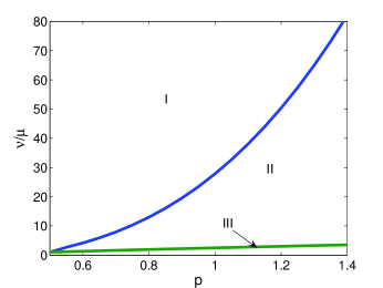
Figure 1: Phase diagram over stable parameter region in $p$. The region I phase is MFT level pattern formation, the region II phase is noise driven pattern formation and quasi-cycles and region III is a spatially homogeneous phase with quasi-cycles.

An additional feature of the model is that oscillations and spatial pattern formation are essentially decoupled. This means that the model predicts global population oscillations and spatial pattern formation, but not traveling waves. The mathematical origin of this can be seen in Eq. 7. The $k^{2}$ term with a negative coefficient at $\omega=0$ is quickly overwhelmed by the positive $k^{2}$ dependence of the $\omega^{2}$ term as the frequency begins to grow. In the power spectrum (fig. 2) this can be seen as the deep valley between the peaks in $k$ and $\omega$. This interpretation is supported by preliminary simulations of an agent based model.

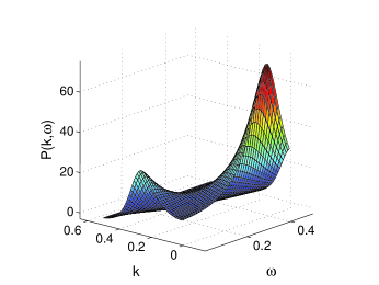
Figure 2: Power spectrum with p=1, $\nu/\mu$=15

We also note that the appropriate thermodynamic limit of the theory is not $V\rightarrow\infty$, but rather that the number of patches of size $V$ goes to infinity. Since $V$ is the volume of a locally well mixed population, it should never be infinity for a system in which diffusion effects are significant. Thus the results we have presented do not depend on the size of the population being studied, and even apply to infinite populations, provided local populations are finite. In ecological terms, this means that systems in which fluctuation effects might be expected to be insignificant due to large populations (e.g. plankton) are equally likely to contain fluctuation driven patterns and cycles as systems with small populations, at least over length scales where diffusion is a reasonable approximation for the spatial dynamics.

The results we have given here were calculated within a specific model, but we expect that they will be substantially unchanged in any model with a slow diffusing activator species and a faster diffusing inhibitor species.

This work was partially supported by National Science Foundation grant NSF-EF-0526747.

References

- Turing (1953) A. M. Turing, Phil. Trans. Roy. Soc. B 237, 37 (1953).
- Maron and Harrison (1997) J. L. Maron and S. Harrison, Science 278, 1619 (1997).
- Reitkerk and van de Koppel (2008) M. Reitkerk and J. van de Koppel, TREE 23, 169 (2008).
- Levin and Segel (1976) S. A. Levin and L. A. Segel, Nature 259, 659 (1976).
- Malchow et al. (1998) H. Malchow, F. M. Hilker, I. Siekmann, S. Petrovski, and A. B. Medvinsky, Aspects of Mathematical Modelling pp. 1–26 (1998).
- Davis et al. (1992) C. S. Davis, S. M. Gallager, and A. R. Solow, Science 257, 230 (1992).
- Abraham (1998) E. R. Abraham, Nature 391, 577 (1998).
- Mimura and Murray (1978) M. Mimura and J. D. Murray, J. Theor. Biol. 75, 249 (1978).
- Baurmann et al. (2007) M. Baurmann, T. Gross, and U. Feudel, J. Theor. Biol. 245, 220 (2007).
- Mobilia et al. (2006) M. Mobilia, I. T. Georgiev, and U. C. Tauber, Phys. Rev. E 73, 040903(R) (2006).
- Wilson et al. (1999) W. G. Wilson, S. P. Harrison, A. Hastings, and K. McCann, J. Anim. Ecol. pp. 94–107 (1999).
- Maynard Smith (1974) J. Maynard Smith (1974).
- Davis et al. (2008) S. Davis, P. Trapman, H. Leirs, M. Begon, and J. A. P. Heesterbeek, Nature 454, 634 (2008).
- Katori et al. (1998) M. Katori, S. Kizaki, Y. Terui, and T. Kubo, Fractals 6, 81 (1998).
- McKane and Newman (2005) A. J. McKane and T. J. Newman, Phys. Rev. Lett. 94, 218102 (2005).
- Pineda-Krch et al. (2007) M. Pineda-Krch, H. J. Blok, and M. Doebeli, Oikos 116, 53 (2007).
- Lugo and McKane (2008) C. Lugo and A. J. McKane, Phys. Rev. E 78 (2008).
- Butler and Reynolds (2009) T. Butler and D. Reynolds, Phys. Rev. E 79, 032901 (2009).
- Courchamp et al. (1999) F. Courchamp, T. Clutton-Brock, and B. Grenfell, TREE 14, 405 (1999).
- Wilson (1998) W. G. Wilson, The American Naturalist 151, 116 (1998).
- García-Ojalvo et al. (1993) J. García-Ojalvo, A. Hernández-Machado, and J. M. Sancho, Phys. Rev. Lett. 71, 1542 (1993).
- Carrillo et al. (2004) O. Carrillo, S. M. A, G.-O. J, and J. M. Sancho, Europhys. Lett. 65, 452 (2004).
- Sieber et al. (2007) M. Sieber, H. Malchow, and L. Schimansky-Geier, Ecological complexity 4, 223 (2007).
- Doi (1976) M. Doi, J. Phys. A. 9, 1465 (1976).
- Goldenfeld (1984) N. Goldenfeld, J. Phys. A 17, 2807 (1984).
- Mikhailov (1981) A. S. Mikhailov, Phys. Lett. 85, 214 (1981).
- Peliti (1985) L. Peliti, PJ. Physique 46, 1469 (1985).
- Janssen and Tauber (2005) H. K. Janssen and U. C. Tauber, Annals of Physics 315, 147 (2005).
- Van Kampen (1992) N. G. Van Kampen, Stochastic Processes in Physics and Chemistry (Elsevier, New York, 1992).
- Martin et al. (1973) P. C. Martin, E. D. Siggia, and H. A. Rose, Phys. Rev. A 8, 423 (1973).
- Bausch et al. (1976) R. Bausch, H. K. Janssen, and H. Wagner, Z. Phys. B. 24, 113 (1976).