’t Hooft-Polyakov monopoles in lattice SU($N$)+adjoint Higgs theory

Abstract

We investigate twisted C-periodic boundary conditions in SU($N$) gauge field theory with an adjoint Higgs field. We show that with a suitable twist for even $N$ one can impose a non-zero magnetic charge relative to residual U(1) gauge groups in the broken phase, thereby creating a ’t Hooft-Polyakov magnetic monopole. This makes it possible to use lattice Monte-Carlo simulations to study the properties of these monopoles in the quantum theory.

I Introduction

’t Hooft-Polyakov monopoles ’t Hooft (1974); Polyakov (1974) play an important role in high energy physics, partly because their existence as physical particles is a general prediction of grand unified theories, and partly because they provide a way to study non-perturbative properties of quantum field theories through electric-magnetic dualities Montonen and Olive (1977). Most of the existing studies of monopoles in non-supersymmetric theories have been restricted to the level of classical solutions, and little is known about quantum mechanical effects. Calculation of even leading-order quantum corrections to solitons is hard, and can usually only be done in simple one-dimensional models Dashen et al. (1974).

Lattice Monte Carlo simulations provide an alternative, fully non-perturbative approach Ciria and Tarancon (1994). However, because of their non-perturbative nature, they always describe the true ground state of the system and therefore do not allow one to specify a background about which the theory is quantised.

There are two general approaches to calculating properties of monopoles and other solitons in Monte Carlo simulations. One can either define suitable creation and annihilation operators and measure their correlators Veselov et al. (1996); Del Debbio et al. (1995); Frohlich and Marchetti (1999), or one can impose boundary conditions that restrict the path integral to a non-trivial topological sector Smit and van der Sijs (1991). The former approach is closer in spirit to usual Monte Carlo simulations and in principle it gives access to a wide range of observables including, e.g., the vacuum expectation value of the monopole field. However, because monopoles are surrounded by a spherical infinite-range magnetic Coulomb field, it is difficult to find a suitable operator and separate the true ground state from excited states.

Instead, while non-trivial boundary conditions provide access to a more limited set of observables, they ensure that the monopole is always in its ground state. Early attempts to simulate monopoles were based on fixed boundary conditions Smit and van der Sijs (1994), but this introduced large finite-size effects. To avoid them, one needs to use boundary conditions that are periodic up to the symmetries of the theory. Such boundary conditions were introduced for the SU($2$) theory in Ref. Davis et al. (2000), and they were used to calculate the mass of the monopoles in Refs. Davis et al. (2002); Rajantie (2006).

In this paper, we generalise this result to SU($N$) gauge group with $N>2$. This is important for several reasons. Many analytical results are only valid in the large-$N$ limit, and for grand unified theory monopoles one needs SU($5$) or larger groups. The SU($2$) group is also somewhat special, and a richer theoretical structure with new questions arises when one goes beyond it. For instance, there can be several different monopole species and unbroken non-Abelian gauge groups.

We find that as in the SU($2$) theory, monopoles can be created by boundary conditions that consist of complex conjugation and a topological non-trivial gauge transformation, but only for even $N$. The boundary conditions treat all monopole species in the same way, so we cannot single out one for creation. Instead of actually fixing the magnetic charge, we can only choose between odd and even charges. However, even with these limitations, the boundary conditions make it possible to measure the monopole mass.

The paper is organsied as follows. In Sections II and III, we review the definitions of the magnetic field and magnetic charge in the SU($N$)+adjoint Higgs theory in the continuum and on the lattice, respectively. In Section IV we show how the monopole mass is expressed in terms of partion functions for different topological sectors. In Section V, we introduce twisted C^∗-periodic boundary conditions and show that they can be used to calculate the monopole mass.

II Magnetic charges in the continuum

The most general renormalisable Lagrangian for the SU($N$) gauge field theory $A_{\mu}$ with an adjoint Higgs field $\Phi$ is

$${\cal L} = -{\rm Tr}G^{\mu\nu}G_{\mu\nu}+{\rm Tr}[D_{\mu},\Phi][D^{\mu},\Phi]$$ (1)

$$-m^{2}{\rm Tr}\Phi^{2}-\kappa{\rm Tr}\Phi^{3}-\lambda_{1}({\rm Tr}\Phi^{2})^{2}-\lambda_{2}{\rm Tr}\Phi^{4},$$

where we have used the covariant derivative and field strength tensor defined by

$$D_{\mu}=\partial_{\mu}+igA_{\mu},\quad G_{\mu\nu}=-\frac{i}{g}[D_{\mu},D_{\nu}],$$ (2)

respectively. Both $\Phi$ and $A_{\mu}$ are Hermitian and traceless $N\times N$ matrices, which can be expanded in terms of the group generators $T^{A}$,

$$\Phi(x)=\phi^{A}(x)T^{A},\quad A_{\mu}(x)=A_{\mu}^{A}(x)T^{A},$$ (3)

with real coefficients $\phi^{A}$ and $A_{\mu}^{A}$. The fields can therefore also be thought of as $N^{2}-1$ component vectors.

Let us first consider the case $N=2$. In this case the group generators can be chosen to be the Pauli matrices,

$$T^{A}=\frac{\sigma^{A}}{2}.$$ (4)

Because of the properties of the Pauli matrices, ${\rm Tr}\Phi={\rm Tr}\Phi^{3}=0$ and $({\rm Tr}\Phi^{2})^{2}=2{\rm Tr}\Phi^{4}$, and therefore we can choose $\kappa=\lambda_{2}=0$ without any loss of generality.

In the broken phase, where $m^{2}<0$, the Higgs field has a vacuum expectation value

$$\langle{\rm Tr}\Phi^{2}\rangle=\frac{1}{2}\langle\phi^{A}\phi^{A}\rangle=\frac{v^{2}}{2}\equiv\frac{m^{2}}{\lambda}.$$ (5)

The SU($2$) symmetry is spontaneously broken to U($1$). To represent the direction of symmetry breaking, we define

$$\hat{\Phi}(x)=\frac{\Phi(x)}{\sqrt{2{\rm Tr}\Phi(x)^{2}}},$$ (6)

which is well defined whenever $\Phi\neq 0$. Following ’t Hooft ’t Hooft (1974), we use this to define the field strength

$$F_{\mu\nu} = 2{\rm Tr}\hat{\Phi}G_{\mu\nu}-\frac{4i}{g}{\rm Tr}\hat{\Phi}[D_{\mu},\hat{\Phi}][D_{\nu},\hat{\Phi}]$$

$$= \partial_{\mu}(\hat{\phi}^{A}A_{\nu}^{A})-\partial_{\nu}(\hat{\phi}^{A}A_{\mu}^{A})+\frac{\epsilon_{ABC}}{g}\hat{\phi}^{A}(\partial_{\mu}\hat{\phi}^{B})\partial_{\mu}\hat{\phi}^{C}.$$

Fixing the unitary gauge, in which $\Phi\propto\sigma^{3}$, makes this definition more transparent. The gauge fixing is achieved by the gauge transform $R(x)$, such that the transformed field $\tilde{\Phi}$ is diagonal

$$\tilde{\Phi}(x)\equiv R^{\dagger}(x)\Phi(x)R(x)=\sqrt{2{\rm Tr}\Phi^{2}}\frac{\sigma^{3}}{2}.$$ (8)

In terms of the transformed gauge field

$$\tilde{A}_{\mu}=R^{\dagger}A_{\mu}R-\frac{i}{g}R^{\dagger}\partial_{\mu}R,$$ (9)

the field strength tensor has the usual Abelian form,

$$F_{\mu\nu}=\partial_{\mu}\tilde{A}_{\nu}^{3}-\partial_{\nu}\tilde{A}_{\mu}^{3}.$$ (10)

Alternatively, we can express this in terms of the diagonal elements of the transformed gauge field,

$$F_{\mu\nu}^{a}=\partial_{\mu}\tilde{A}_{\nu}^{aa}-\partial_{\nu}\tilde{A}_{\mu}^{aa}.$$ (11)

This defines a two-component vector of field strength tensors, but tracelessness of $A_{\mu}$ implies $F_{\mu\nu}^{2}=-F_{\mu\nu}^{1}$. The conventional field strength $F_{\mu\nu}$ is given by $F_{\mu\nu}=F_{\mu\nu}^{1}-F_{\mu\nu}^{2}$.

The conserved magnetic current corresponding to the residual U(1) group is defined as

$$j_{\mu}^{a}=\partial^{\nu}{}^{\star}F_{\mu\nu}^{a},$$ (12)

where ${}^{\star}F_{\mu\nu}^{a}$ is the dual tensor,

$${}^{\star}F_{\mu\nu}^{a}=\frac{1}{2}\epsilon_{\mu\nu\rho\sigma}F^{a\,\rho\sigma}.$$ (13)

Like the field strength, the magnetic currents satisfy $j_{\mu\nu}^{2}=-j_{\mu\nu}^{1}$, so there is only one monopole species.

Substituting Eq. (II), one finds

$$j_{\mu}^{1}=\frac{1}{4g}\epsilon_{\mu\nu\rho\sigma}\epsilon_{ABC}(\partial^{\nu}\hat{\phi}^{A})(\partial^{\rho}\hat{\phi}^{B})(\partial^{\sigma}\hat{\phi}^{C})=-j_{\mu}^{2}.$$ (14)

This clearly vanishes when $\Phi\neq 0$, but is generally non-zero when $\Phi$ vanishes. The magnetic charge inside volume $V$ bounded by a closed surface $S$ that encloses a zero is

$$Q=\int_{V}d^{3}xj_{0}=\pm\frac{2\pi}{g}(1,-1).$$ (15)

This can be generalized to SU($N$) ’t Hooft (1981). The matrices $\{T^{A}\}$ in Eq. (3) are now the generators of SU($N$) in the fundamental representation, and we assume the usual normalisation

$${\rm Tr}T^{A}T^{B}=\frac{1}{2}\delta^{AB}.$$ (16)

As in Eq. (8), consider a gauge transformation $R(x)$ that diagonalizes $\Phi(x)$ and places the eigenvalues in descending order,

$$\tilde{\Phi}(x)=R^{\dagger}(x)\Phi(x)R(x)=\text{diag}(\lambda_{1},...,\lambda_{N}),$$ (17)

where $\lambda_{1}\geq\lambda_{2}\geq...\geq\lambda_{N}$.

In classical field theory one usually finds that there are only two distinct eigenvalues, and consequently only one residual U(1) group. In that case one can use Eq. (II) to define the corresponding field strength. However, as we will discuss in Section III, in lattice Monte Carlo simulations all the eigenvalues are distinct. In that case, $\tilde{\Phi}(x)$ is invariant under gauge transformations generated by the $N-1$ diagonal generators of SU($N$). Thus we are left with a residual U(1)^N-1 gauge invariance corresponding the Cartan subgroup of SU($N$). It is then convenient to follow ’t Hooft ’t Hooft (1981) and define the residual U(1) field strengths by Eq. (11), with $a\in\left\{1,\ldots,N\right\}$. The corresponding magnetic currents $j_{\mu}^{a}$ are then given by Eq. (12). They satisfy the tracelessness condition

$$\sum_{a=1}^{N}F_{\mu\nu}^{a}=\sum_{a=1}^{N}j_{\mu\nu}^{a}=0,$$ (18)

so that there are only $N-1$ independent U(1) fields and magnetic charges.

In three dimensions any two eigenvalues coincide, $\lambda_{b}=\lambda_{b+1}$, in a discrete set of points, which behave like magnetic charges with respect to the components $F^{b}_{\mu\nu}$ and $F^{b+1}_{\mu\nu}$ of the field strength tensor (11) ’t Hooft (1981). That is, it behaves like a magnetic monopole with charge $Q=\pm\hat{q}_{b}$, where the elementary magnetic charges are

$$\hat{q}_{b}^{a}=\frac{2\pi}{g}\left(\delta_{a,b}-\delta_{a,(b+1)}\right),$$ (19)

or in vector notation

$$\hat{q}_{b}=\frac{2\pi}{g}\left(\overbrace{0,...,0}^{b-1},1,-1,\overbrace{0,...,0}^{N-b-1}\right).$$ (20)

In the core of the monopole, the SU($2$) subgroup involving the $b$th and $(b+1)$th components of the fundamental representation is restored.

III Magnetic charge on the lattice

On the lattice, the Higgs field is defined on sites $x$ while the gauge degrees of freedom are encoded in SU($N$) valued link variables $U_{\mu}(x)$. The Lagrangian is given by

$${\cal L} = \frac{1}{g^{2}}\sum_{\mu\nu}{\rm Tr}U_{\mu}({x})U_{\nu}(x+\hat{\mu})U_{\mu}^{\dagger}({x}+\hat{\nu})U_{\nu}^{\dagger}({x})$$ (21)

$$+2\sum_{\mu}\left[{\rm Tr}\Phi({x})^{2}-{\rm Tr}\Phi({x})U_{\mu}({x})\Phi({x}+\hat{\mu})U_{\mu}^{\dagger}({x})\right]$$

$$+m^{2}{\rm Tr}\Phi^{2}+\kappa{\rm Tr}\Phi^{3}+\lambda_{1}({\rm Tr}\Phi^{2})^{2}+\lambda_{2}{\rm Tr}\Phi^{4}.$$

Again, we diagonalise $\Phi$ by a gauge transformation $R(x)$,

$$\tilde{\Phi}(x)=R^{\dagger}(x)\Phi(x)R(x).$$ (22)

Link variables are transformed to

$$\tilde{U}_{\mu}(x)=R^{\dagger}(x)U_{\mu}(x)R(x+\hat{\mu}).$$ (23)

The diagonalised field $\tilde{\Phi}$ is still invariant under diagonal gauge transformations,

$$D(x) = {\rm diag}\,(e^{i\Delta_{1}(x)},\ldots,e^{i\Delta_{N}(x)}),$$ (24)

$$\sum_{a=1}^{N}\Delta_{a}=0\mod\leavevmode\nobreak\ 2\pi,$$

which form the residual U(1)^N-1 symmetry group and contain the elements of the center $\mathbb{Z}_{N}$ of SU($N$).

To identify the corresponding U(1) field strength tensors, we need to decompose $\tilde{U}_{\mu}$ Kronfeld et al. (1987),

$$\tilde{U}_{\mu}(x)=C_{\mu}(x)u_{\mu}(x),$$ (25)

where $u_{\mu}(x)$ represents the residual U(1) gauge fields and transforms as

$$u_{\mu}(x)\rightarrow D^{\dagger}(x)u_{\mu}(x)D(x+\hat{\mu}),$$ (26)

and $C_{\mu}(x)$ represents fields charged under the U(1) groups. This decomposition is not unique Kronfeld et al. (1987). A simple choice is to define Abelian link variables as the diagonal elements of $\tilde{U}_{\mu}$ in direct analogy with Eq. (11),

$$u_{\mu}(x)={\rm diag}\,\tilde{U}_{\mu}(x).$$ (27)

In practice, it is often more convenient to work with link angles and define an $N$-component vector

$$\alpha_{\mu}^{a}(x)=\arg u_{\mu}^{aa}.$$ (28)

As angles, these are only defined modulo $2\pi$, and we choose them to be in the range $-\pi<\alpha_{\mu}^{a}\leq\pi$. As in the continuum, the angles $\alpha_{\mu}^{a}$ satisfiy

$$\sum_{a}\alpha_{\mu}^{a}(x)=0\leavevmode\nobreak\ \mod\leavevmode\nobreak\ 2\pi.$$ (29)

Therefore it has only $N-1$ independent components, corresponding to the $N-1$ residual U(1) gauge groups.

Next, we construct plaquette angles as

$$\alpha_{\mu\nu}^{a}(x)=\alpha_{\mu}^{a}(x)+\alpha_{\nu}^{a}(x+\hat{\mu})-\alpha_{\mu}^{a}(x+\hat{\nu})-\alpha_{\nu}^{a}(x),$$ (30)

which are the lattice analogs of the Abelian field strength. In the continuum limit, they are related by

$$F_{\mu\nu}^{a}=\frac{1}{g}\alpha_{\mu\nu}.$$ (31)

Because the links $\alpha_{\mu}^{a}$ are only defined modulo $2\pi$, the same applies to the plaquette, and again, we choose $-\pi<\alpha_{\mu\nu}^{a}\leq\pi$.

Using Eq. (30), the corresponding lattice magnetic currents are

$$j_{\mu}^{a}=\frac{1}{g}\Delta_{\nu}^{f}\ {}^{\star}\alpha_{\mu\nu}^{a},$$ (32)

where $\Delta_{\nu}^{f}$ is the forward derivative in direction $\nu$ on the lattice and

$$\ {}^{\star}\alpha_{\mu\nu}^{a}=\frac{1}{2}\epsilon_{\mu\nu\rho\sigma}\alpha_{\rho\sigma}^{a}.$$ (33)

These are integer multiples of $2\pi$, because each contribution of $\alpha_{\mu}^{a}(x)$ is cancelled by a $-\alpha_{\mu}^{a}(x)$ modulo $2\pi$.

In particular, the Abelian magnetic charge inside a single lattice cell is given by

$$q^{a}(x)=j_{0}^{a}=\frac{1}{2g}\sum_{ijk}\epsilon_{ijk}\left(\alpha_{ij}^{a}(x+\hat{k})-\alpha_{ij}^{a}(x)\right).$$ (34)

Each component of this vector is an integer multiple of $(2\pi/g)$, and they all add up to zero. The elementary charges, corresponding to individual monopoles, are the same as in the continuum (20). Other values of the charge vector $q$ correspond to composite states made of elementary monopoles.

The diagonalisation procedure in Eq. (17) is ill defined whenever the Higgs field has degenerate eigenvalues, but on lattice the set of field configurations in which that happens has zero measure in the path integral. Physically this means that the core of the monopole never lies exactly at a lattice site. Therefore these configurations do not contribute to any physical observable and do not have to be considered separately.

IV Monopole mass

The Abelian magnetic charge $Q$ of any lattice field configuration is well defined by adding up the contributions (34) from each lattice cell,

$$Q=\sum_{x}q(x).$$ (35)

Because it is discrete, one can define separate partition functions $Z_{Q}$ for each magnetic charge sector. The full partition function is simply the product

$$Z=\prod_{Q}Z_{Q}.$$

The ground state energy of a given charge sector may be defined by

$$E_{Q}=-\frac{1}{T}\ln\frac{Z_{Q}}{Z_{0}},$$ (36)

where $Z_{0}$ is the partition function of the charge zero sector and $T$ is the length of the lattice in the time direction. The mass $M_{j}$ of a single monopole $\hat{q}_{j}$ is given by the ground state energy of the corresponding charge sector

$$M_{j}=E_{\hat{q}_{j}}.$$ (37)

In order to calculate the energies $E_{Q}$, we need to impose boundary conditions that enforce non-trivial Abelian magnetic charge. It is important that these boundary conditions preserve the translational invariance of the system, because otherwise our calculations are tainted by boundary effects. Because they are generally proportional to the surface area they would completely swamp the contribution from a point-like monopole which we want to measure.

Gauss’s law rules out periodic boundary conditions since they fix the charge to zero. However, translational invariance only requires periodicity up to the symmetry of the Lagrangian (21). Since the magnetic current is conserved, we need only consider spatial boundary conditions.

For SU($2$), it was found in Davis et al. (2000) that the following boundary conditions force an odd value for the magnetic charge,

$$\Phi(x+L\hat{\jmath}) = -\sigma_{j}\Phi(x)\sigma_{j}=(\sigma_{2}\sigma_{j})^{\dagger}\Phi^{*}(x)(\sigma_{2}\sigma_{j}),$$

$$U_{\mu}(x+L\hat{\jmath}) = \sigma_{j}U_{\mu}(x)\sigma_{j}=(\sigma_{2}\sigma_{j})^{\dagger}U_{\mu}^{*}(x)(\sigma_{2}\sigma_{j}).$$

These are an example of twisted C-periodic boundary conditions, as introduced by Kronfeld and Wiese Kronfeld and Wiese (1991). Note that while twisted C-periodic and twisted periodic boundary conditions are equivalent for the gauge links, the Higgs field requires an additional anti-periodicity when we convert from one form to the other. Physically, this means that charge conjugation is carried only by the Higgs field in SU($2$). We will come back to this important point when we discuss the boundary conditions in terms of the flux sectors of pure SU($2$) gauge theory.

In contrast, it turns out that untwisted C-periodic boundary conditions,

$$\Phi(x+L\hat{\jmath}) = -\sigma_{2}\Phi(x)\sigma_{2}=\Phi^{*}(x)$$

$$U_{\mu}(x+L\hat{\jmath}) = \sigma_{2}U_{\mu}(x)\sigma_{2}=U_{\mu}^{*}(x),$$ (38)

are compatible with any even value of magnetic charge Davis et al. (2000) but are locally gauge equivalent to the twisted ones (IV). Assuming that monopoles do not form bound states, the weight of the multi-monopole configurations in the path integral is exponentially suppressed

$$Z_{Q}=e^{-MT}Z_{0},$$ (39)

where $M$ is the monopole mass and $T$ is the temporal size of the lattice. In the infinite-volume limit, $T\rightarrow\infty$, only the configurations with the minimum number of monopoles contribute to the path integral. So the partition function $Z_{{\rm odd}}$ for twisted C-periodic boundary conditions will be dominated by configurations with a single monopole, while the partition function $Z_{{\rm even}}$ will be dominated by configurations with no monopoles. Therefore the monopole mass is given by

$$M=-\lim_{T\rightarrow\infty}\frac{1}{T}\ln Z_{{\rm odd}}/Z_{{\rm even}}.$$ (40)

This was used to calculate the non-perturbative mass of the ’t Hooft-Polyakov monopole in Davis et al. (2002); Rajantie (2006), with good agreement with classical expectations.

V Twisted boundary conditions

Let us now generalise the boundary conditions (IV) to SU($N$) with $N>2$. To avoid boundary effects, the boundary conditions must preserve translation invariance, and they will therefore have to be periodic up to the symmetries of the theory. In the case of Eq. (21), the available symmetries are complex conjugation of the fields and gauge invariance. When $\kappa=0$, reflection of the Higgs field $\Phi\rightarrow-\Phi$ is also a symmetry, but in general it is not, and therefore we do not consider it. The appropriate extension of (IV) is then a combination of complex conjugation and gauge transformations.

V.1 Fully C-periodic boundary conditions

It is natural to impose complex conjugation in all three spatial directions, in which case we have

$$\Phi(x+L\hat{\jmath}) = \Omega_{j}^{\dagger}(x)\Phi^{*}(x)\Omega_{j}(x),$$

$$U_{\mu}(x+L\hat{\jmath}) = \Omega_{j}^{\dagger}(x)U_{\mu}^{*}(x)\Omega_{j}(x+\hat{\mu}),$$ (41)

where the SU($N$) gauge transformation matrix $\Omega_{j}(x)$ can in general be position dependent. We refer to these as (fully) C-periodic boundary conditions Kronfeld and Wiese (1991).

To avoid contradiction at the edges, it should not matter in which order the boundary conditions are applied. Therefore, the gauge transformations must satisfy Kronfeld and Wiese (1991)

$$\begin{split}\Omega_{j}^{\dagger}&(x+L\hat{k})\Omega_{k}^{T}(x)\Phi(x)\Omega_{k}^{*}(x)\Omega_{j}(x+L\hat{k})\\ &=\Phi(x+L\hat{\jmath}+L\hat{k})\\ &=\Omega_{k}^{\dagger}(x+L\hat{\jmath})\Omega_{j}^{T}(x)\Phi(x)\Omega_{j}^{*}(x)\Omega_{k}(x+L\hat{\jmath}),\end{split}$$ (42)

and

$$\begin{split}\Omega_{j}^{\dagger}&(x+L\hat{k})\Omega_{k}^{T}(x)U_{\mu}(x)\Omega_{k}^{*}(x+\hat{\mu})\Omega_{j}(x+L\hat{k}+\hat{\mu})\\ &=U_{\mu}(x+L\hat{\jmath}+L\hat{k})\\ &=\Omega_{k}^{\dagger}(x+L\hat{\jmath})\Omega_{j}^{T}(x)U_{\mu}(x)\Omega_{j}^{*}(x+\hat{\mu})\Omega_{k}(x+L\hat{\jmath}+\hat{\mu}).\end{split}$$ (43)

Since our fields are blind to center elements, Eq. (42) implies the cocycle condition

$$\Omega_{i}^{*}(x)\Omega_{j}(x+L\hat{\imath}) = z_{ij}\,\Omega_{j}^{*}(x)\Omega_{i}(x+L\hat{\jmath}),$$

$$z_{ij} = e^{i\theta_{ij}},$$ (44)

where the $N$th roots of unity $z_{ij}=z_{ji}^{*}$ are formed by the antisymmetric ’twist tensor’ $\theta_{ij}=-\theta_{ji}$ with the usual parametrisation in terms of three $\mathbb{Z}_{N}$-valued numbers $m_{i}$,

$$\theta_{ij}=\frac{2\pi}{N}\,\epsilon_{ijk}m_{k},\quad m_{i}\in\mathbb{Z}_{N}.$$ (45)

Furthermore, Eq. (43) implies that the $z_{ij}$ have to be independent of position.

All choices of $\Omega_{i}(x)$, $\Omega_{j}(x)$ with the same twist $z_{ij}$ are gauge equivalent ’t Hooft (1979); Kronfeld and Wiese (1991), and we therefore assume that we can choose the matrices $\Omega_{j}$ to be independent of position analogous to the standard ‘twist eaters’ in the case of ’t Hooft’s twisted boundary conditions without charge conjugation Ambjorn and Flyvbjerg (1980). Explicit realisations for the allowed C-periodic twists Kronfeld and Wiese (1991) by constant $\Omega$’s for even $N$ are straightforward and will be given in Sec. V.3 below.

The fact that non-trivial twists with C-periodic boundary conditions are only possible for even $N$ can be seen explicitly by considering the effect of the cocycle condition (44) on the product $\Omega_{i}\Omega_{j}^{*}\Omega_{k}$ Kronfeld and Wiese (1991). On one hand, we have

$$\Omega_{i}\Omega_{j}^{*}\Omega_{k} = z_{jk}\Omega_{i}\Omega_{k}^{*}\Omega_{j}$$ (46)

$$= z_{jk}z_{ki}\Omega_{k}\Omega_{i}^{*}\Omega_{j}$$

$$= z_{jk}z_{ki}z_{ij}\Omega_{k}\Omega_{j}^{*}\Omega_{i},$$

but applying the condition in the opposite order we find

$$\Omega_{i}\Omega_{j}^{*}\Omega_{k} = z_{ji}\Omega_{j}\Omega_{i}^{*}\Omega_{k}$$ (47)

$$= z_{ji}z_{ik}\Omega_{j}\Omega_{k}^{*}\Omega_{i}$$

$$= z_{ji}z_{ik}z_{kj}\Omega_{k}\Omega_{j}^{*}\Omega_{i}.$$

Therefore the twist tensors must satisfy the constraint

$$z_{ji}^{2}z_{jk}^{2}z_{ki}^{2}=1,$$ (48)

which implies for the $\mathbb{Z}_{N}$ valued $m_{i}$, that

$$\mbox{\small${\displaystyle\frac{2}{N}}$}(m_{1}+m_{2}+m_{3})\in\{0,1\}.$$ (49)

Hence, for non-trivial C-periodic twist, $N/2$ must be in $\mathbb{Z}_{N}$, i.e. $N$ must be even Kronfeld and Wiese (1991).

Let us now consider the effect of the boundary conditions (41) on the residual U(1) fields. Because the eigenvalues of the Higgs field $\Phi$ don’t change under the twists in (41), i.e. $\Phi(x)$ and $\Phi(x+L\hat{\jmath})$ have the same set of eigenvalues, which are all real, we can choose the diagonalised field $\tilde{\Phi}$ defined in Eq. (22) to be periodic,

$$\tilde{\Phi}(x+L\hat{\jmath})=\tilde{\Phi}(x).$$ (50)

Then, on one hand,

$$\Phi({x}+L\hat{\jmath}) = \Omega_{j}^{\dagger}\Phi^{*}({x})\Omega_{j}$$ (51)

$$= \Omega_{j}^{\dagger}\left(R({x})\tilde{\Phi}({x})R^{\dagger}({x})\right)^{*}\Omega_{j}$$

$$= \Omega_{j}^{\dagger}R^{*}({x})\tilde{\Phi}({x}+L\hat{\jmath})R^{T}({x})\Omega_{j},$$

while on the other,

$$\Phi({x}+L\hat{\jmath})=R({x}+L\hat{\jmath})\tilde{\Phi}({x}+L\hat{\jmath})R^{\dagger}({x}+L\hat{\jmath}).$$ (52)

To ensure the compatibility of the two, we impose spatial boundary conditions for $R(x)$ as follows,

$$R({x}+L\hat{\jmath})=\Omega_{j}^{\dagger}R^{*}({x}).$$ (53)

When we apply multiple translations by $L$, however, we observe $\mathbb{Z}_{N}$ jumps in the definition of gauge transforms $R(x)$ in SU($N$). A double translation by $L$ first along the $k$ direction and then along $j$ for example is defined by

$$R^{jk}({x}+L\hat{\jmath}+L\hat{k})\equiv\Omega_{j}^{\dagger}\Omega_{k}^{T}R({x}),$$ (54)

while for a translation first along $j$ followed by one in the $k$ direction leads to

$$R^{kj}({x}+L\hat{\jmath}+L\hat{k})\equiv\Omega_{k}^{\dagger}\Omega_{j}^{T}R({x}),$$ (55)

From (44) it then immediately follows that

$$R^{jk}({x}+L\hat{\jmath}+L\hat{k})=z_{kj}R^{kj}({x}+L\hat{\jmath}+L\hat{k}).$$ (56)

From their effect in (22), or generally in SU($N$)$/\mathbb{Z}_{N}$, these two would be equivalent. In SU($N$) they are not, however. There, transformations where the $R^{\prime}s$ applied at a corner site to links in different directions attached to that corner differ, by center elements as in (56), can be used to change the twist sector. If we allowed such multi-valued, and hence singular gauge transformations, we could then arrange matters such that the transformed link variables $\tilde{U}$ would all be C-periodic,

$$\tilde{U}_{\mu}({x}+L\hat{\jmath}) = R^{\dagger}({x}+L\hat{\jmath})U_{\mu}({x}+L\hat{\jmath})R({x}+\hat{\mu}+L\hat{\jmath})$$ (57)

$$= R^{T}({x})U_{\mu}^{*}({x})R^{*}({x}+\hat{\mu})$$

$$= \tilde{U}_{\mu}^{*}({x}).$$

The twist would then be completely removed by the singular gauge transformation, however. Conversely, when comparing a fundamental Wilson loop that winds around a plane with non-trivial twist to the corresponding loop formed by the $\tilde{U}$’s, one would observe that the original loop obtained its center flux entirely from the $\mathbb{Z}_{N}$ jump of the multi-valued gauge transformation, while the $\tilde{U}$ loop, with purely C-periodic b.c.’s (57), would be trivial.

In order to preserve the $\mathbb{Z}_{N}$ center flux in SU($N$), we must apply single-valued and hence proper SU($N$) gauge transformations, without such a jump. Those will of course not change the Wilson loop at all, when transforming the $U$’s to the gauge-fixed links $\tilde{U}$. Then however, we have to decide how we define the gauge transformation at those corner sites where $\mathbb{Z}_{N}$ ambiguities as in (56) arise. Consequently, the boundary conditions (57) for the gauge-fixed $\tilde{U}$’s attached to such a corner will have to be amended.

This is best exemplified in two dimensions (with two integer coordinates $x$ and $y$ both ranging from $0$ to $L-1$): At the site with coordinates $(L,L)$ we define the gauge transformation $R$ as, say

$$R(L,L)\equiv\Omega_{y}^{\dagger}\Omega_{x}^{T}R(0,0)=\Omega_{y}^{\dagger}R^{*}(L,0).$$ (58)

If we consider the $x$ link attached to this corner site, we obtain the boundary condition

$$\tilde{U}_{x}(L-1,L) = R^{\dagger}(L-1,L)U_{x}(L-1,L)R(L,L)$$ (59)

$$= R^{T}(L-1,0)U_{x}^{*}(L-1,0)R^{*}(L,0)$$

$$= \tilde{U}_{x}^{*}(L-1,0),$$

as in (57) and as for every other link that is not connected to this corner. For the corresponding $y$ link at this corner on the other hand,

$$\tilde{U}_{y}(L,L-1) = R^{\dagger}(L,L-1)U_{y}(L,L-1)R(L,L)$$ (60)

$$\hskip-56.9055pt=R^{T}(0,L-1)U_{y}^{*}(0,L-1)\Omega_{x}\Omega_{y}^{\dagger}\Omega_{x}^{T}R^{*}(0,0)$$

$$\hskip-56.9055pt=z_{21}\,R^{T}(0,L-1)U_{y}^{*}(0,L-1)R^{*}(0,L)$$

$$\hskip-56.9055pt=z_{21}\,\tilde{U}_{y}^{*}(0,L-1),$$

because $\Omega_{y}^{\dagger}\Omega_{x}^{T}=z_{21}\Omega_{x}^{\dagger}\Omega_{y}^{T}$ and $R^{*}(0,L)=\Omega_{y}^{T}R(0,0)$. This shows that all but one of the gauge-fixed links in the plane are C-periodic (57) and that the center flux comes about by the boundary condition of the one link remaining.

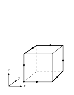
Figure 1: Integration curve used to calculate the flux through half of the box.

In the following we will only consider proper transformations $R$, single-valued in SU($N$), so that the center flux is preserved in the gauge-fixed links, $\tilde{U}$. In higher dimensions we therefore introduce the convention that for gauge transformations $R$ involving multiple translations by $L$ these translations are always applied in lexicographic order. In three dimensions, this leads to the following definitions for the far edges of our $L^{3}$ box with one corner in the origin at (0,0,0),

$$R(L,L,z) \equiv \Omega^{\dagger}_{y}\Omega^{T}_{x}R(0,0,z),$$

$$R(L,y,L) \equiv \Omega^{\dagger}_{z}\Omega^{T}_{x}R(0,y,0),$$

$$R(x,L,L) \equiv \Omega^{\dagger}_{z}\Omega^{T}_{y}R(x,0,0),$$ (61)

where $x$, $y$ and $z$ run from $0$ to $L-1$; and for the corner diagonally opposite to the origin, we use

$$R(L,L,L)\,\equiv\,\Omega^{\dagger}_{z}\Omega^{T}_{y}\Omega^{\dagger}_{x}R^{*}(0,0,0).$$ (62)

In particular, we then have

$$R(L,L,L)=z_{12}z_{23}z_{31}\Omega^{\dagger}_{x}\Omega^{T}_{y}\Omega^{\dagger}_{z}R^{*}(0,0,0),$$ (63)

and the factor

$$z_{12}z_{23}z_{31}=\exp\big{\{}\mbox{\small${\displaystyle\frac{2\pi i}{N}}$}(m_{1}+m_{2}+m_{3})\big{\}}$$ (64)

represents the total center flux as measured by a maximal-size Wilson loop $W(C)$ along the corners of the three-dimensional cube that cuts its surface into two equal halfs as in Fig. 1. To see this, let the loop $C$ in Fig. 1 be composed of two line segments $-\gamma_{1}$ and $\gamma_{2}$ as shown in Fig. 2, for example, and consider gauge transforming the two Wilson lines $W(\gamma_{1})$ and $W(\gamma_{2})$. To make them equal, so that $W(C)=W(\gamma_{2})W^{\dagger}(\gamma_{1})=1$, we would need to apply a gauge transform

$$R^{(1)}(L,L,L)=\Omega^{\dagger}_{z}\Omega^{T}_{y}\Omega^{\dagger}_{x}R^{*}(0,0,0)$$

at the end of line $W(\gamma_{1})$, but

$$R^{(2)}(L,L,L)=\Omega^{\dagger}_{x}\Omega^{T}_{y}\Omega^{\dagger}_{z}R^{*}(0,0,0)$$

at the end of $W(\gamma_{2})$. This would be a multi-valued gauge transform with a jump at the far corner at $(L,L,L)$, however. If we apply the same $R(L,L,L)\equiv R^{(1)}(L,L,L)$ at the end of both lines, $W(\gamma_{1})$ and $W(\gamma_{2})$, the loop $W(C)$ remains unchanged, and we have,

$$W(C)=W(\gamma_{2})W^{\dagger}(\gamma_{1})=z_{12}z_{23}z_{31}\ .$$ (65)

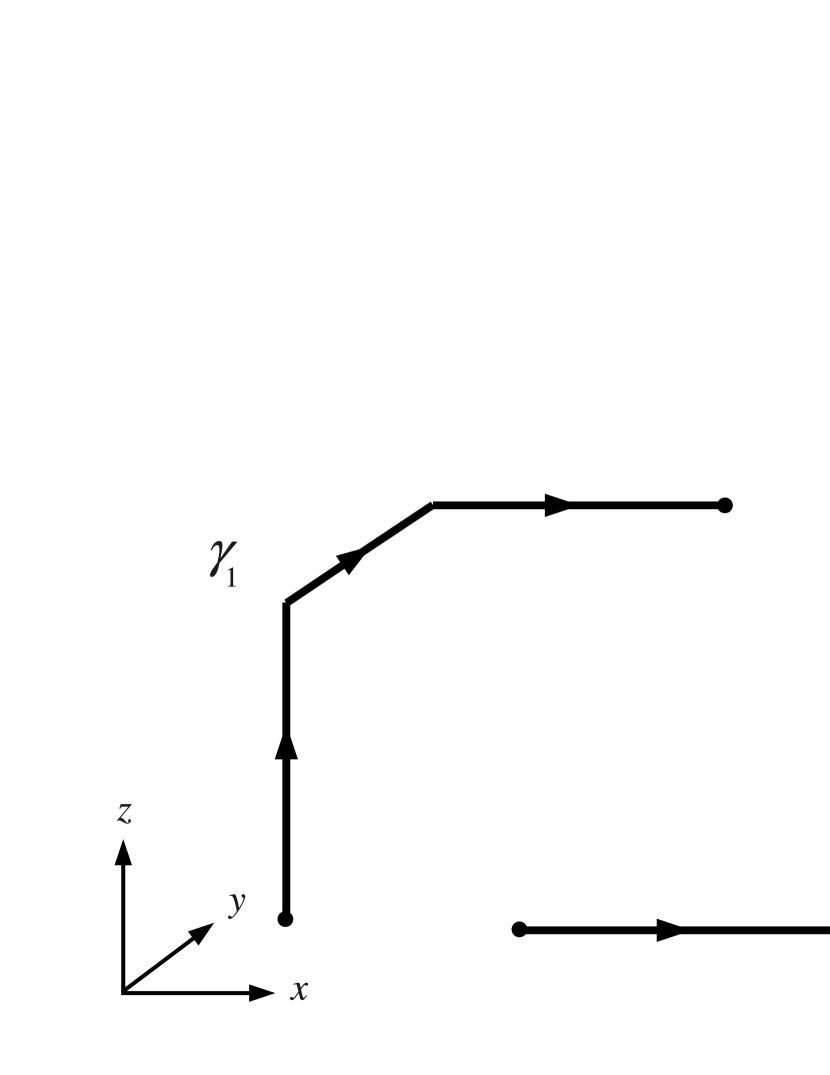
Figure 2: Two line segments $\gamma_{1}$ and $\gamma_{2}$ that can be used to compose the loop in Fig. 1.

In terms of the gauge-fixed links $\tilde{U}$, we then still have C-periodic boundary conditions (57) for most of the links, but we need to take into account the following exceptions:

$$\tilde{U}_{y}(L,L-1,z) = z_{21}\,\tilde{U}_{y}^{*}(0,L-1,z),$$

$$\tilde{U}_{z}(L,y,L-1) = z_{31}\,\tilde{U}_{z}^{*}(0,y,L-1),$$

$$\tilde{U}_{z}(x,L,L-1) = z_{32}\,\tilde{U}_{z}^{*}(x,0,L-1),$$ (66)

where the third variable runs from 0 to $L-1$ again; and, from the corner at $(L,L,L)$,

$$\tilde{U}_{y}(L,L-1,L) = z_{12}\,\tilde{U}_{y}(0,L-1,0),$$ (67)

$$\tilde{U}_{z}(L,L,L-1) = z_{32}z_{13}\,\tilde{U}_{z}(0,0,L-1).$$

The set of special links whose boundary conditions are modified by center elements is sketched in Fig. 3.

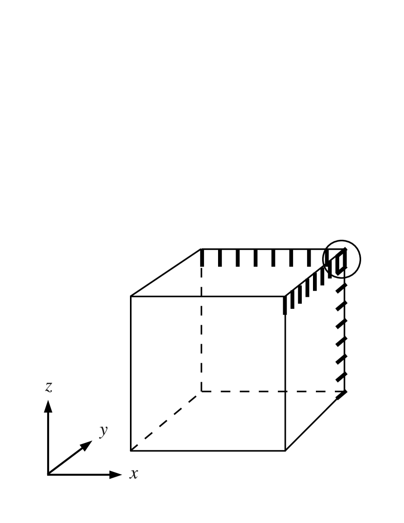
Figure 3: Illustration of links with special boundary conditions in three dimensions. When center flux is moved to the upper right plaquettes of all two dimensional planes, it piles up near the corner at $(L,L,L)$ as highlighted by the circle.

Along the loop of Fig. 1 this means that almost every link in the first half of the loop has a partner in the opposite direction in the second half, to which it is related by two successive C-periodic translations (57), and hence periodic. There are only two exceptions from the set of twisted links that the loop picks up. These are

$$\tilde{U}_{y}(L,L-1,0) = z_{21}\tilde{U}_{y}^{*}(0,L-1,0)$$

$$= z_{21}\tilde{U}_{y}(0,L-1,L),$$

and the last link of the first half of the loop which ends at the corner at $(L,L,L)$, as given in (67),

$$\tilde{U}_{z}(L,L,L-1)=z_{32}z_{13}\tilde{U}_{z}(0,0,L-1).$$ (69)

The combined center elements are again responsible for the same total center flux through the loop, now in terms of the gauge-fixed links, $\tilde{U}$.

V.2 Magnetic flux

If the decomposition (25) commutes with complex conjugation, which (27) does, the boundary conditions (41) imply anti-periodicity of the $\alpha_{\mu}^{a}(x)$ in (28). Therefore the Abelian projected fields inherit anti-periodic boundary conditions

$$\alpha_{\mu}^{a}({x}+L\hat{\jmath})=-\alpha_{\mu}^{a}({x}),$$ (70)

except for the special cases, in three dimensions corresponding to the links in Eqs. (66), where

$$\alpha_{y}^{a}(L,L-1,z) = -\alpha_{y}^{a}(0,L-1,z)-\mbox{\small${\displaystyle\frac{2\pi}{N}}$}\,m_{3},$$ (71)

$$\alpha_{z}^{a}(L,y,L-1) = -\alpha_{z}^{a}(0,y,L-1)+\mbox{\small${\displaystyle\frac{2\pi}{N}}$}\,m_{2},$$

$$\alpha_{z}^{a}(x,L,L-1) = -\alpha_{z}^{a}(x,0,L-1)-\mbox{\small${\displaystyle\frac{2\pi}{N}}$}\,m_{1},$$

and in Eqs. (67), where

$$\alpha_{y}^{a}(L,L-1,L) = \alpha_{y}^{a}(0,L-1,0)+\mbox{\small${\displaystyle\frac{2\pi}{N}}$}\,m_{3},$$ (72)

$$\alpha_{z}^{a}(L,L,L-1) = \alpha_{z}^{a}(0,0,L-1)-\mbox{\small${\displaystyle\frac{2\pi}{N}}$}\,(m_{1}+m_{2}).$$

It can be verified that the fluxes in three dimensions,

$$\alpha_{ij}^{a}(\vec{x})=\alpha_{i}^{a}(\vec{x})+\alpha_{j}^{a}(\vec{x}+\hat{\imath})-\alpha_{i}^{a}(\vec{x}+\hat{\jmath})-\alpha_{j}^{a}(\vec{x})$$ (73)

are all essentially anti-periodic, because the twist angles $(2\pi/N)m_{i}$ cancel when we compare fluxes on opposite sides of the lattice. There is a single exception here also, however, for which we obtain,

$$\alpha_{23}(L,L-1,L-1) =$$

$$\hskip-85.35826pt-\alpha_{23}(0,L-1,L-1)-\mbox{\small${\displaystyle\frac{2\pi}{N}}$}\,2(m_{1}+m_{2}+m_{3}).$$

Because of the constraint on the possible twists in Eq. (49), and because flux is only defined modulo $2\pi$, the additional contribution has no effect, and this is equivalent to anti-periodic boundary conditions also. We therefore have fully anti-periodic Abelian field strengths. This means that when we cross the boundary we enter a charge conjugated copy of the same lattice from the opposite side.

To determine the magnetic charge we repeat the trick of Davis et al. (2000). The curve shown in Figure 1 divides the boundary into two halves. We denote the magnetic flux through them by $\Phi_{+}$ and $\Phi_{-}$ choosing the positive direction to be pointing outwards. The two halves are related by the boundary conditions, and in particular, the antiperiodicity (73) of the field strength implies that they are equal $\Phi_{-}=\Phi_{+}$. The magnetic charge inside the lattice is given by the total flux, which is the sum of the two contributions, which means

$$Q=\Phi_{+}+\Phi_{-}=2\Phi_{+}.$$ (75)

Applying Stokes’s theorem, we can write

$$\Phi_{+}^{a} = -\frac{1}{g}\left(\sum_{x=0}^{L-1}\alpha_{x}^{a}(x,0,0)+\sum_{y=0}^{L-1}\alpha_{y}^{a}(L,y,0)\right.$$ (76)

$$\left.+\sum_{z=0}^{L-1}\alpha_{z}^{a}(L,L,z)-\sum_{x=0}^{L-1}\alpha_{1}^{a}(x,L,L)\right.$$

$$\left.-\sum_{y=0}^{L-1}\alpha_{y}^{a}(0,y,L)-\sum_{z=0}^{L-1}\alpha_{3}^{a}(0,0,z)\right).$$

When we apply the boundary conditions, all terms cancel except those involving the cases,

$$\Phi_{+}^{a} = -\frac{1}{g}\left(\alpha_{y}^{a}(L,L-1,0)+\alpha_{z}^{a}(L,L,L-1)\right.$$ (77)

$$\hskip 14.22636pt\left.-\alpha_{y}^{a}(0,L-1,L)-\alpha_{z}^{a}(0,0,L-1)\right)$$

$$= \frac{1}{g}\frac{2\pi}{N}\left(m_{1}+m_{2}+m_{3}\right).$$

where we have used the first equation in (71) with $z=0$ and $\alpha_{y}^{a}(0,L-1,0)=-\alpha_{y}^{a}(0,L-1,L)$, and the second equation in (72).

Because the link angles $\alpha_{\mu}^{a}$ are defined modulo $2\pi$, the fluxes $\Phi_{\pm}$ are only defined modulo $(2\pi/g)$. Therefore we find

$$Q^{a}=\frac{4\pi}{gN}(m_{1}+m_{2}+m_{3})\mod\leavevmode\nobreak\ \frac{4\pi}{g}.$$ (78)

V.3 Allowed magnetic charges

It is obvious from Eq. (78) that the possible charges one can create using the boundary conditions is quite restricted. As in the continuum (20), the components are quantised in units of $2\pi/g$. Substituting the constraint on the twists for even $N$ in Eq. (49) into Eq. (78) gives the charge quantisation condition

$$Q^{a}=\frac{2\pi}{g}\,\mathbb{Z}_{2},$$ (79)

up to integer multiples of $(4\pi/g)$. Because all components of the charge vector $Q^{a}$ are furthermore the same, modulo $(4\pi/g)$, we then automatically satisfy the constraint,

$$\sum_{a}Q^{a}=NQ_{a}=0\mod\leavevmode\nobreak\ \frac{4\pi}{g}.$$ (80)

In summary, this means that we can use twised C-periodic boundary conditions in SU($N$), when $N$ is even, to restrict the ensemble to either of two distinct classes of monopole configurations. If the allowed twists satisfy $m_{1}+m_{2}+m_{3}=0$ (modulo $N$), then their total charges are all integer multiples of $(4\pi/g)$,

$$Q^{a}=0\mod\leavevmode\nobreak\ \frac{4\pi}{g}\leavevmode\nobreak\ \mbox{for all $a$}.$$ (81)

If the twists are such that $m_{1}+m_{2}+m_{3}=N/2$ on the other hand, every component of the total charge vector is a half-odd integer multiple of $(4\pi/g)$,

$$Q^{a}=\frac{2\pi}{g}\mod\leavevmode\nobreak\ \frac{4\pi}{g}\leavevmode\nobreak\ \mbox{for all $a$}.$$ (82)

Those two sectors differ by at least one unit of Abelian magnetic charge $(2\pi/g)$ (modulo $(4\pi/g)$) in each of the $N-1$ U($1$)’s. This may be due to a single monopole in a diagonally embedded U($1$) or due to several monopoles in different U($1$)’s depending on the symmetry breaking pattern. If the symmetry breaking is maximal, these could be $N-1$ individual monopoles, one in every U($1$) factor of the maximal Abelian subgroup of SU($N$). Because $N$ must be even, the total number of monopoles in the twisted sector will be odd in either case. The ratio of partition functions of the two sectors in the infinite volume limit determines the free energy of such monopole configurations or, at zero temperature, their total mass as discussed in Section IV.

For even $N$, we can therefore force an odd number of monopoles in each residual $U(1)$ by imposing boundary conditions that correspond to Eq. (82). A convenient choice is

$$\begin{array}[]{c}\Omega_{1}=\text{diag}(i\sigma_{3},...,i\sigma_{3})\\ \Omega_{2}=\text{diag}(I,...,I)\\ \Omega_{3}=\text{diag}(i\sigma_{1},...,i\sigma_{1}).\end{array}$$ (83)

These are simply the SU(2) matrices from Eq. (IV) repeated in block diagonal form. They satisfy

$$\Omega_{i}^{*}\Omega_{j}=-\Omega_{j}^{*}\Omega_{i},\;i\neq j,$$ (84)

corresponding to a $\pi$ twist angle in each plane, i.e. $m_{1}=m_{2}=m_{3}=N/2$. We could equally well use a a single twisted plane by replacing $\Omega_{1}$ or $\Omega_{3}$ by the unit matrix $1$. An even number of monopoles, corresponding to Eq. (81), is of course obtained by simply choosing

$$\Omega_{1}=\Omega_{2}=\Omega_{3}=1.$$ (85)

We have therefore found that the twisted boundary conditions (41) allow us to impose a non-zero magnetic charge, but with several restrictions. It is, in fact, fairly natural that we cannot specify the exact charge but only whether it is odd or even with boundary conditions that preserve translational invariance Polley and Wiese (1991).

The other restriction, that all charges must have the same value, arises because our boundary conditions are linear operations on the fields. The transformation matrices $\Omega_{j}$ are therefore independent of the direction of symmetry breaking $\Phi$, which defines the different residual U(1) groups. Therefore the boundary conditions cannot treat any U(1) group differently from the others. It may be possible to avoid this restriction by considering non-linear transformations. In principle, one could specify the boundary conditions in the unitary gauge in which the different U(1) groups can be treated separately. However, it is not clear if it is possible even then to impose translation invariant boundary conditions that give different values to different magnetic charges.

In summary, the boundary conditions (41) allow us to define the partition functions $Z_{{\rm odd}}$ and $Z_{{\rm even}}$ in Eq. (40) using the gauge transformation (83) and (85), respectively. Using Eq. (40), we can therefore calculate the energy difference between these two sectors.

If there is only one residual U(1) group, which is usually the case, only the monopole species that corresponds to it is massive, and therefore Eq. (40) gives that monopole’s mass, just as in SU(2). If there are several residual U(1) groups, there is a magnetic charge corresponding to each U(1) group, and therefore $Z_{{\rm odd}}$ generally represents a multi-monopole state. Depending on which configuration has the lowest energy, the monopoles may either be separate free particles, in which case Eq. (40) gives the sum of their masses, or as a bound state in which case it gives the energy of the bound state.

V.4 Mixed boundary conditions

In the previous subsection, we imposed complex conjugation in all three directions. This has the advantage of preserving the invariance of the theory under 90-degree rotations. However, for a non-zero magnetic charge, it is enough to have complex conjugation in one direction, so that the flux can escape through at least one face, and we can ask whether that would lead to fewer restrictions for the allowed magnetic charges. In Appendix A we show that this is not the case, and that even for such “mixed” boundary conditions, the allowed magnetic charges are constrained exactly as in Section V.3.

With a single C-periodic direction, for example, we find in App. A.1 that the outward fluxes, $\Phi^{\parallel}_{\pm}$, parallel to this direction and through the perpendicular faces at opposite sides of the volume are equal, and quantised in terms of the magnetic center flux $m_{\parallel}$ in that direction,

$$\Phi_{+}^{\parallel}=\Phi_{-}^{\parallel}=\mbox{\small${\displaystyle\frac{2\pi}{gN}}$}\,m_{\parallel}\;.$$ (86)

In contrast, the Abelian fluxes in the two orthogonal directions are no-longer quantised, but they are both conserved,

$$\Phi_{+}^{\perp}+\Phi_{-}^{\perp}=0\;.$$ (87)

So there is one extra source of strength $2m_{\parallel}/N$ in units of magnetic charge $(2\pi/g)$ whose entire flux goes along the C-periodic direction,

$$Q=\Phi_{+}^{\parallel}+\Phi_{-}^{\parallel}=\mbox{\small${\displaystyle\frac{2\pi}{g}}$}\,\mbox{\small${\displaystyle\frac{2m_{\parallel}}{N}}$}\;,$$ (88)

again modulo $(4\pi/g)$ and the same for all $a=1,\dots N-1$. But as we show in the Appendix, we again have

$$\mbox{\small${\displaystyle\frac{2m_{\parallel}}{N}}$}\,\in\{0,1\},$$ (89)

which again restricts the construction to even $N$, because $2m_{\parallel}/N$ is also an element of the center, $\mathbb{Z}_{N}$.

It is instructive to compare this to the case of standard twisted boundary conditions, without any C-periodic direction, where the analogously defined Abelian projected fluxes are all quantised and conserved, i.e. where

$$\Phi^{(i)}_{+}=-\Phi_{-}^{(i)}=\mbox{\small${\displaystyle\frac{1}{g}}$}\mbox{\small${\displaystyle\frac{2\pi}{N}}$}\,m_{i}\;,\;\;\mbox{for all}\;i=1,2,3.$$ (90)

The introduction of one C-periodic direction thus led to non-quantised contributions of Abelian projected flux in the orthogonal directions in addition to the center flux (90) of the corresponding sectors with standard twists a la ’t Hooft, c.f. Eqs. (111) and (112). These non-quantised contributions are due to the Abelian projection and may not have any physical significance at all. So unlike standard center flux, the flux in the orthogonal directions is no-longer quantised, but like standard center flux it is still conserved.

In contrast, the flux along the C-periodic direction is still quantised in units of center elements, see Eqs. (109) and (110), but it is no-longer conserved. The introduction of the C-periodic direction has led to a reversal of the center flux when passing through the volume along this direction, by introducing a source of a strength of twice that magnetic flux into the volume, c.f. Eq. (88).

But this only works for center fluxes with $-m=m$, which can be non-trivial only when $-1$ is among the roots of unity and $N$ is even. Then however, these particular fluxes are $\mathbb{Z}_{2}$ valued and do not have a direction. In the pure gauge theory we cannot even distinguish positive from negative flux in this case, which is why we can reverse it without harm in the first place. So for the pure gauge theory we have gained nothing new here. Moreover, ’t Hooft’s magnetic fluxes as employed here play no role in the deconfinement transition of the pure gauge theory, the free energy of the corresponding center vortices always vanishes in the thermodynamic limit von Smekal and de Forcrand (2003).

But together with our adjoint Higgs fields, which have anti-periodic Abelian components in such a C-periodic direction, we can distinguish the relative orientations of center vortex and Higgs field as described in Sec. VI.2 below. And together with the adjoint Higgs field, the different magnetic sectors have now become relevant – not for confinement in the pure gauge theory, but for the masses of ’t Hooft-Polyakov monopoles and the Higgs mechanism.

VI Relation to vortices

VI.1 The continuum and zeroes of the Higgs field for SU($2$)

It would be nice to see how the boundary conditions (41) relate to magnetic charge in the continuum theory. This is straightforward when the gauge group is SU($2$). In this case, Abelian monopoles are located at zeroes of the Higgs field. So to have an odd number of monopoles we must have an odd number of zeroes of $\Phi$. To proceed, it’s helpful to write the boundary conditions in the form

$$\Phi(x+L\hat{\jmath})=-\sigma_{j}\Phi(x)\sigma_{j}.$$ (91)

It’s then clear that the components of the Higgs field in the adjoint representation $\Phi={\phi}^{A}{\sigma}^{A}/2$ inherit the conditions

$$\phi^{1}(x+L\hat{x}) = -\phi^{1}(x),$$

$$\phi^{2}(x+L\hat{y}) = -\phi^{2}(x),$$

$$\phi^{3}(x+L\hat{z}) = -\phi^{3}(x),$$ (92)

with all other components periodic. This respects a ’hedgehog’ configuration, as it should.

Note, for example, that $\phi^{1}$ must have an odd number of zeroes on every line through the box in the $x$ direction. By continuity, these combine to form surfaces pinned to the boundary of the othogonal plane. Similarly, there must be an odd number of surfaces through the $y$ and $z$ directions where $\phi^{2}$ and $\phi^{3}$ are respectively zero. Because of their relative orthogonality, these surfaces intersect in an odd number of points where all three components are zero. To help picture this, consider the surfaces where $\phi^{1}$ and $\phi^{2}$ are zero. These intersect to form an odd number of lines in the $z$ direction on which $\phi^{1}$ and $\phi^{2}$ are both zero. Since $\phi^{3}$ is antiperiodic in the $z$ direction, there must be an odd number of points on these lines (and in total) where ${\phi}^{A}$ vanishes.

All of the (partial or mixed) C-periodic boundary conditions that force an odd magnetic charge have this property. Conversely, those with trivial magnetic charge modulo $4\pi$ are found to permit only an even number points where the Higgs field is zero.

VI.2 Vortex picture - Laplacian center gauge

As we’ve seen, the allowed Abelian magnetic charges are tightly connected to and restricted by the center flux sectors of the pure gauge theory. Here the relevant objects are center vortices, which are strings of center flux in three dimensions, and surfaces in four dimensions.

It is commonly believed that colour confinement is the result of certain topological objects that dominate the QCD vacuum on large distance scales, and center vortices are a leading candidate Greensite (2003). In the vortex picture of confinement, Wilson loops acquire a ’disordering’ phase factor from every vortex that they link with Greensite (2003). The area law for timelike Wilson loops in pure SU($N$) gauge theory comes from the percolation of spacelike vortex sheets in the confined phase. Their free energies have been measured over the deconfinement phase transition in the pure SU(2) gauge theory with methods entirely analogous to the ones described here, from ratios of partition functions with twisted boundary conditions in temporal planes forcing odd numbers of $\mathbb{Z}_{2}$ center vortices through those planes over the periodic ensemble with even numbers de Forcrand and von Smekal (2002); von Smekal and de Forcrand (2002). A Kramers-Wannier duality is then observed by comparing the behaviour of these center vortices with that of ’t Hooft’s electric fluxes which yield the free energies of static charges in a well-defined (UV-regular) way de Forcrand and von Smekal (2002), with boundary conditions to mimic the presence of ’mirror’ (anti)charges in neighbouring volumes. This duality follows that between the Wilson loops of the 3-dimensional $\mathbb{Z}_{2}$-gauge theory and the 3d-Ising spins, reflecting the universality of the center symmetry breaking transition.

This is in contrast to the monopole scenario, where confinement is attributed to the dual Meissner effect from a monopole condensate. It turns out that these descriptions may be complimentary, at least in certain gauges. In the last few years it’s become clear that monopole world lines are embedded on the surface of center vortices Ambjorn et al. (2000); Chernodub et al. (2005); de Forcrand and Pepe (2001); Reinhardt (2002); Cornwall (2000, 1998, 2002). Percolation of one implies percolation of the other. From this perspective, we can regard center vortices as Abelian vortices, sourced by the monopoles. For SU($2$) gauge theory, the monopoles are like beads on a necklace. For general SU($N$), several center vortices may meet at a point and we instead have monopole-vortex nets. Similar objects have been found in various supersymmetric gauge theories containing Higgs fields Tong (2009).

With this in mind, it’s interesting to reinterpret our results from the point of view of vortices. This is particularly instructive for SU($2$), where there is no distinction between twisted C-periodic and twisted periodic boundary conditions for the gauge degrees of freedom Kronfeld and Wiese (1991). The gauge content of our configurations can therefore be interpreted in terms of twisted periodic boundary conditions, where the vortex structure is well understood. Twist in a plane corresponds to an odd number of center vortices piercing that plane ’t Hooft (1979).

In this case, charge conjugation is carried entirely by the Higgs field. We will see how a C-periodic/antiperiodic Higgs field modifies the vortex structure of pure SU($2$) gauge theory and leads to Abelian magnetic charge. We will then generalise to SU($N$).

First we need a way of locating center vortices, which are generally thick objects. This proceeds via gauge fixing and center projection. A common choice in the pure gauge theory is Maximal Center Gauge followed by a projection of the link variables onto the ’nearest’ center element Greensite (2003). The resultant excitations are thin $\mathbb{Z}_{N}$ vortices known as P-vortices. These are expected to signal the location of center vortices in the unprojected configurations. However, since we have a Higgs field at our disposal it makes more sense to use a modified version of Laplacian Center Gauge Vink and Wiese (1992); van der Sijs (1997, 1998); de Forcrand and Pepe (2001). After diagonalising $\Phi$ we’re left with a residual U(1)^N-1 gauge symmetry. The idea of Laplacian Center Gauge is to use the lowest-lying eigenvector of the adjoint Laplacian operator as a faux Higgs field. We can reduce the gauge symmetry to $\mathbb{Z}_{N}$ by fixing $N-1$ phases of this auxialary field. Thin vortices then arise a la Nielsen-Olesen.

We’ll follow the construction of de Forcrand and Pepe de Forcrand and Pepe (2001) which starts from the adjoint lattice Laplacian,

$$\begin{split}&-\Delta_{xy}^{AB}({U})\\ &=\sum_{\mu}(2\delta_{x,y}\delta^{AB}-{U}_{\mu}^{AB}(x)\delta_{y,x+\hat{\mu}}-{U}_{\mu}^{BA}(x-\hat{\mu})\delta_{y,x-\hat{\mu}}),\end{split}$$ (93)

where $A,B$ are the colour indices, $x,y$ the lattice coordinates, and ${U}_{\mu}^{AB}$ the link variables in the adjoint representation,

$${U}_{\mu}^{AB}(x)=2\text{Tr}(T^{A}U_{\mu}(x)T^{B}U_{\mu}^{\dagger}(x)).$$ (94)

Since $\Delta$ is a real symmetric matrix, its eigenvalues are real. If we take $\lambda_{1}$ to be the smallest eigenvalue, the corresponding eigenvector allows us to associate a real 3-dimensional vector $\phi_{(1)}^{A}(x)$ with each lattice site. The eigenvalues of $\Delta$ are invariant under gauge transformations $R(x)$, and $\phi_{(1)}^{A}$ transforms like an adjoint scalar field de Forcrand and Pepe (2001), with $\Phi_{(1)}(x)=\phi_{(1)}^{A}(x)T^{A}$,

$$\Phi_{(1)}(x)\rightarrow\tilde{\Phi}_{(1)}(x)=R^{\dagger}(x)\Phi_{(1)}(x)R(x).$$ (95)

After diagonalising the physical Higgs field, the transformed field $\tilde{\Phi}_{(1)}(x)$ will not in general be invariant under remnant U(1)^N-1 transformations. The gauge freedom may then be reduced to $\mathbb{Z}_{N}$ by eliminating the phases of all $(N-1)$ sub-diagonal elements. Gauge ambiguities arise when any of the sub-diagonal elements of $\tilde{\Phi}_{(1)}(x)$ are zero. This involves two conditions, so gauge ambiguities form lines in three dimensions. Since they carry quantised center flux, these defects are identifed as $\mathbb{Z}_{N}$ vortices de Forcrand and Pepe (2001).

For SU($2$), note that we have a $\mathbb{Z}_{2}$ vortex whenever ${\phi}_{(1)}^{A}(x)$ is parallel or antiparallel to the physical Higgs field in colour space. The relative sign of ${\phi}_{(1)}^{A}(x)$ and the Higgs gives its local orientation. In the neighbourhood of a monopole, the Higgs field has a hedgehog shape in colour space. So there is necessarily some direction along which ${\phi}_{(1)}^{A}(x)$ and the Higgs field are collinear. What’s more, their relative orientation changes sign at the location of the Abelian charge. It follows that every monopole lies on a thin $\mathbb{Z}_{2}$ vortex, which appears as two oppositely directed strings. Monopoles and anti-monopoles form an alternating bead-like structure on the vortices. See de Forcrand and Pepe (2001) for more details and the generalization to SU($N$).

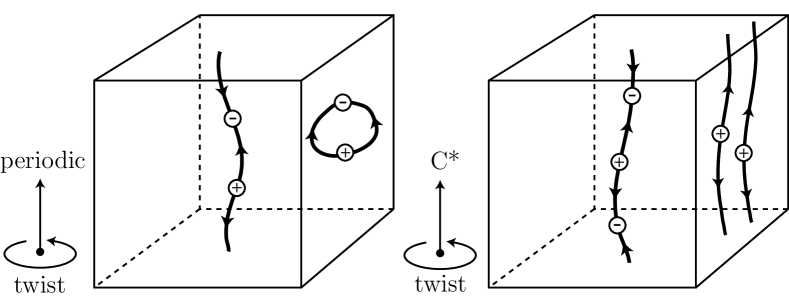
Figure 4: For SU($2$), Abelian monopoles form a bead-like structure on center vortices. To have odd net charge we need an odd number of vortices that contain an odd number of monopoles. i.e. both twist and charge conjugation.

How does this relate to our boundary conditions? Let’s start with SU($2$). Recall that twisted C-periodic and twisted periodic boundary conditions are equivalent for the gauge links. Twist in a plane forces an odd number of $\mathbb{Z}_{2}$ vortices through that plane. For each of these to contribute an odd number of monopoles/anti-monopoles, the orientation of $\mathbb{Z}_{2}$ flux should change an odd number of times. Therefore ${\phi}^{A}{\phi}^{A}_{(1)}=2\text{Tr}\Phi\Phi_{(1)}$ should be antiperiodic. The boundary conditions

$$\Phi(x+L\hat{\jmath}) = \pm\Omega_{j}^{\dagger}(x)\Phi(x)\Omega_{j}(x),$$

$$U_{\mu}(x+L\hat{\jmath}) = \Omega_{j}^{\dagger}(x)U_{\mu}(x)\Omega_{j}(x+\hat{\mu}),$$ (96)

give

$$\begin{split}2\text{Tr}&\Phi(x+N\hat{\jmath})\Phi^{(1)}(x+N\hat{\jmath})\\ &=\pm 2\text{Tr}\Omega_{j}^{\dagger}\Phi(x)\Omega_{j}\Omega_{j}^{\dagger}\Phi^{(1)}(x)\Omega_{j}\\ &=\pm 2\text{Tr}\Phi(x)\Phi^{(1)}(x).\end{split}$$ (97)

So if the Higgs field is antiperiodic/C-periodic, $2\text{Tr}\Phi\Phi_{(1)}$ is also antiperiodic, and there will be an odd number of monopoles on every vortex in that direction.

The net magnetic charge is then obtained from simple counting arguments. Closed vortices and vortices through periodic directions do not contribute, since they contain an equal number of monopoles and anti-monopoles. And without twist we can only have an even number of monopoles, since there will be an even number of vortices. For the net charge to be odd, there must be an odd number of directions that are both conjugated and have twist in the orthogonal plane. We then have an odd number of vortices that contain an odd number of monopoles. This interpretation is in perfect agreement with the results of Sec. V.3 and the Appendix.

For the generalisation to SU($N$), it’s helpful to start with a single C-periodic direction. The main difference now is that several $\mathbbm{Z}_{N}$ vortices are permitted to meet at a point. We may have monopole-vortex nets as opposed to the necklaces of SU($2$). However, as shown in the Appendix and discussed in Sec. V.4, the center flux through the C-periodic direction is eliminated for odd $N$ and still restricted to $\mathbbm{Z}_{2}$ for even $N$. This is because the center flux, when viewed as Abelian flux, must be equal and opposite at the boundary.

The reversal of flux means that the allowed magnetic charges are governed by

$$\exp{\frac{igQ}{2}}=\exp{i\pi\frac{2m_{\parallel}}{N}},$$ (98)

where $Q$ is an $N$-vector. The formation of monopole-vortex nets is reflected in the various solutions for $Q$. The constituent charges will generally be scattered around the box, connected by vortices that conserve center flux at each monopole.

If $2m_{\parallel}/N=1$ then

$$\begin{split}Q=\frac{2\pi}{g}(1,1,\dots,1-N)+\frac{2\pi}{g}2(n_{1},n_{2},\dots,-\sum_{i=1}^{N-1}n_{i}).\end{split}$$ (99)

That is, the net always contains an odd number of each monopole species. Of course, this is only possible for even $N$. If $2m_{\parallel}/N=0$ we’re left with the second term and hence an even number of each monopole species. Note that this decomposition also applies when all directions are charge conjugated, since by Eqs. (49) and (65) we have the same possibilities for center (and hence Abelian) flux through each half of the box.

VII Conclusions

We have shown how twisted C-periodic boundary conditions (41) consisting of complex conjugation and gauge transformations can be used to impose a non-zero magnetic charge in SU($N$)+adjoint Higgs theory while preserving translation invariance. This generalises the results obtained for SU(2) in Ref. Davis et al. (2000), and makes it possible to study magnetic monopoles in lattice Monte Carlo simulations. In particular, it will be straightforward to measure the monopole mass in the same way as in Ref. Rajantie (2006).

This method has significant restrictions: It only works for SU($N$) with even $N$, the charges can only be constrained to be odd or even, and every residual U(1) group has to have a magnetic charge. Even with these restrictions, the method can be used to study quantum monopoles is new types of systems, for instance in cases where there are several different types of monopoles or an unbroken non-Abelian subgroup. Using methods introduced in Ref. Rajantie and Weir (2009), one should even be able to find the spectrum of different monopole states, including excited states of monopoles.

Appendix A Mixed boundary conditions

A.1 $x$ direction C-periodic, $y,z$ directions periodic

Suppose that we employ boundary conditions with a single C-periodic direction, chosen to be the $x$ direction. These boundary conditions may be written as

$$\Phi(x+L\hat{x})=\Omega_{x}^{\dagger}\Phi^{*}(x)\Omega_{x}, U_{\mu}(x+L\hat{x})=\Omega_{x}^{\dagger}U_{\mu}^{*}(x)\Omega_{x},$$

$$\Phi(x+L\hat{y})=\Omega_{y}^{\dagger}\Phi(x)\Omega_{y}, U_{\mu}(x+L\hat{y})=\Omega_{y}^{\dagger}U_{\mu}(x)\Omega_{y},$$

$$\Phi(x+L\hat{z})=\Omega_{z}^{\dagger}\Phi(x)\Omega_{z}, U_{\mu}(x+L\hat{z})=\Omega_{z}^{\dagger}U_{\mu}(x)\Omega_{z}.$$

Again assuming constant transition funcitons, consistency of the boundary conditions now requires

$$\Omega_{x}\Omega_{y} = z_{12}\Omega_{y}^{*}\Omega_{x},$$

$$\Omega_{x}\Omega_{z} = z_{13}\Omega_{z}^{*}\Omega_{x},$$

$$\Omega_{y}\Omega_{z} = z_{23}\Omega_{z}\Omega_{y},$$ (100)

where $z_{ij}=e^{i\theta_{ij}}$, $\theta_{ij}=(2\pi/N)\,\epsilon_{ijk}m_{k}$ with $m_{k}\in\mathbb{Z}_{N}$, are center elements as before. Note that charge conjugation only ever happens on one side of the equation.

The gauge transformations to diagonalise the Higgs field have the following genuine boundary conditions,

$$R(x+L\hat{x}) = \Omega^{\dagger}_{x}R^{*}(x),$$ (101)

$$R(x+L\hat{y}) = \Omega^{\dagger}_{y}R(x),$$

$$R(x+L\hat{z}) = \Omega^{\dagger}_{z}R(x),$$

and we define the following doubly translated $R$’s at the far edges and corner by lexicographic order,

$$R(L,L,r) \equiv \Omega_{y}^{\dagger}\Omega_{x}^{\dagger}R^{*}(0,0,r),$$ (102)

$$R(L,r,L) \equiv \Omega_{z}^{\dagger}\Omega_{x}^{\dagger}R^{*}(0,r,0),$$

$$R(r,L,L) \equiv \Omega_{z}^{\dagger}\Omega_{y}^{\dagger}R(r,0,0),$$

for $r=0,\dots L-1$, and

$$R(L,L,L)\equiv\Omega^{\dagger}_{z}\Omega^{\dagger}_{y}\Omega^{\dagger}_{x}R^{*}(0,0,0).$$ (103)

It is straightforward to derive the corresponding boundary conditions for the Abelian projected fields (28),

$$\alpha_{i}^{a}(x+L\hat{x}) = -\alpha_{i}^{a}(x),$$

$$\alpha_{i}^{a}(x+L\hat{y}) = \alpha_{i}^{a}(x),$$

$$\alpha_{i}^{a}(x+L\hat{z}) = \alpha_{i}^{a}(x),$$ (104)

with the following exceptions,

$$\alpha_{y}^{a}(L,L-1,r) = -\alpha_{y}^{a}(0,L-1,r)-\mbox{\small${\displaystyle\frac{2\pi}{N}}$}\,m_{3},$$

$$\alpha_{z}^{a}(L,r,L-1) = -\alpha_{z}^{a}(0,r,L-1)+\mbox{\small${\displaystyle\frac{2\pi}{N}}$}\,m_{2},$$

$$\alpha_{z}^{a}(r,L,L-1) = \alpha_{z}^{a}(r,0,L-1)-\mbox{\small${\displaystyle\frac{2\pi}{N}}$}\,m_{1},$$ (105)

$r=0,\dots L-1$, and

$$\alpha_{y}^{a}(L,L-1,L) = -\alpha_{y}^{a}(0,L-1,0)-\mbox{\small${\displaystyle\frac{2\pi}{N}}$}\,m_{3}$$ (106)

$$= -\alpha_{y}^{a}(0,L-1,L)-\mbox{\small${\displaystyle\frac{2\pi}{N}}$}\,m_{3}$$

$$= \alpha_{y}^{a}(L,L-1,0),$$

as well as

$$\alpha_{z}^{a}(L,L,L-1) = -\alpha_{z}^{a}(0,0,L-1)-\mbox{\small${\displaystyle\frac{2\pi}{N}}$}\,(m_{1}-m_{2})$$ (107)

$$= -\alpha_{z}^{a}(0,L,L-1)-\mbox{\small${\displaystyle\frac{2\pi}{N}}$}\,(2m_{1}-m_{2})$$

$$= \alpha_{z}^{a}(L,0,L-1)-\mbox{\small${\displaystyle\frac{2\pi}{N}}$}\,m_{1}.$$

As expected, it follows that the Abelian field strengths $\alpha_{ij}^{a}(x)$ (30) are periodic in the $y$ and $z$ directions, but anti-periodic in the $x$ direction, again with one exception. And that exception is

$$\alpha_{23}(L,L-1,L-1)=-\alpha_{23}(0,L-1,L-1)-\mbox{\small${\displaystyle\frac{2\pi}{N}}$}\,2m_{1}.$$ (108)

It is this single plaquette where our single-valued gauge transformation $R(x)$ has moved the net magnetic flux to. It leads to opposite fluxes each of strength $(2\pi/gN)m_{1}$ through the faces at $x=0$ and $L$ as illustrated in Figure 5. For the total flux along the positive $x$ direction, for example, we obtain

$$\Phi_{+}^{(1)} = -\mbox{\small${\displaystyle\frac{1}{g}}$}\sum_{r=0}^{L-1}\big{(}\alpha_{y}(L,r,0)+\alpha_{z}(L,L,r)$$ (109)

$$\hskip 56.9055pt-\alpha_{y}(L,r,L)-\alpha_{z}(L,0,r)\big{)}$$

$$= \mbox{\small${\displaystyle\frac{1}{g}}$}\mbox{\small${\displaystyle\frac{2\pi}{N}}$}\,m_{1}.$$

Analogously, we obtain for the total flux in the negative $x$ direction at $x=0$,

$$\Phi_{-}^{(1)} = -\mbox{\small${\displaystyle\frac{1}{g}}$}\big{(}\alpha_{z}(0,0,L-1)-\alpha_{z}(0,L,L-1)\big{)}$$ (110)

$$= \mbox{\small${\displaystyle\frac{1}{g}}$}\mbox{\small${\displaystyle\frac{2\pi}{N}}$}\,m_{1}\,=\Phi^{(1)}_{+}.$$

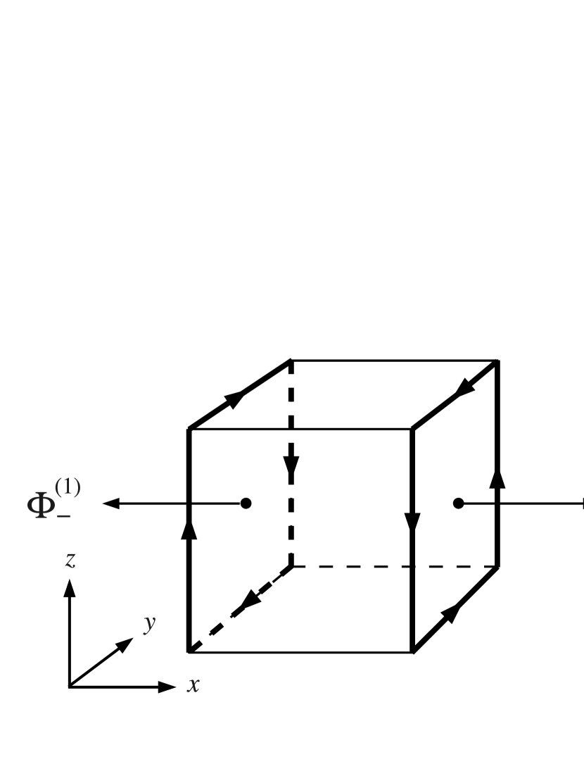
Figure 5: Quantised Abelian fluxes of equal strength in opposite directions, $\Phi^{(1)}_{+}=\Phi^{(1)}_{-}$, with C-periodic $x$ direction.

The analogous Abelian projected fluxes in the $y$ and $z$ directions are not quantised, because they each involve anti-periodic line segments, but they are both conserved. We have

$$\Phi_{+}^{(2)} = -\mbox{\small${\displaystyle\frac{1}{g}}$}\left(2\sum_{r=0}^{L-1}\alpha_{z}(0,0,r)-\mbox{\small${\displaystyle\frac{2\pi}{N}}$}\,m_{2}\right),$$ (111)

$$= -\Phi_{-}^{(2)}$$

and

$$\Phi_{+}^{(3)} = \mbox{\small${\displaystyle\frac{1}{g}}$}\left(2\sum_{r=0}^{L-1}\alpha_{y}(0,r,0)+\mbox{\small${\displaystyle\frac{2\pi}{N}}$}\,m_{3}\right),$$ (112)

$$= -\Phi_{-}^{(3)}$$

Therefore, the Abelian projected fluxes in the $y$ and $z$ directions are not quantised but they are conserved, i.e.

$$\Phi_{+}^{(2)}+\Phi_{-}^{(2)}=\Phi_{+}^{(3)}+\Phi_{-}^{(3)}=0.$$ (113)

There is one extra source of strength $2m_{1}/N$ in units of magnetic charge $(2\pi/g)$ whose entire flux goes along the $x$ direction through the $\alpha_{23}$ plaquettes in the opposite $y=z=L-1$ corners at $x=0$ and $L$,

$$Q=\Phi_{+}^{(1)}+\Phi_{-}^{(1)}=\mbox{\small${\displaystyle\frac{2\pi}{g}}$}\,\mbox{\small${\displaystyle\frac{2m_{1}}{N}}$}\;,$$ (114)

again modulo $(4\pi/g)$ and the same for all $a=1,\dots N-1$.

It would be interesting if the twist angle in the plane perpendicular to the C-periodic direction were permitted to be a phase other than 0 or $\pi$. Unfortunately this is not the case. The proof involves permutations of the twist matrices as before. With C-periodic b.c.’s in the $x$ direction, comparison of

$$\begin{split}\Omega_{x}\Omega_{y}\Omega_{z}&=z_{23}\Omega_{x}\Omega_{z}\Omega_{y}\\ &=z_{23}z_{13}\Omega_{z}^{*}\Omega_{x}\Omega_{y}\\ &=z_{23}z_{13}z_{12}\Omega_{z}^{*}\Omega_{y}^{*}\Omega_{x}\end{split}$$ (115)

with

$$\begin{split}\Omega_{x}\Omega_{y}\Omega_{z}&=z_{12}\Omega_{y}^{*}\Omega_{x}\Omega_{z}\\ &=z_{12}z_{13}\Omega_{y}^{*}\Omega_{z}^{*}\Omega_{x}\\ &=z_{12}z_{13}z_{32}\Omega_{z}^{*}\Omega_{y}^{*}\Omega_{x}\end{split}$$ (116)

yields

$$z_{23}=z_{32}=z_{23}^{*}.$$ (117)

Therefore

$$m_{1}=\begin{cases}0&\text{for odd }N\\ 0\;\text{or}\;N/2&\text{for even }N.\end{cases}$$ (118)

It follows that the allowed charges are exactly those found for fully C-periodic boundary conditions.

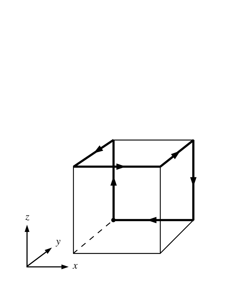
Figure 6: Integration curve for C-periodic $y$ and $z$ directions.

A.2 $y,z$ directions C-periodic, $x$ direction periodic

We can also consider boundary conditions with two C-periodic directions, chosen to be the y and z directions. Then the consistency conditions are modified to

$$\Omega_{x}^{*}\Omega_{y} = z_{12}\Omega_{y}\Omega_{x},$$

$$\Omega_{x}^{*}\Omega_{z} = z_{13}\Omega_{z}\Omega_{x},$$

$$\Omega_{y}^{*}\Omega_{z} = z_{23}\Omega_{z}^{*}\Omega_{y}$$ (119)

with $z_{ij}=e^{i\theta_{ij}}\in\mathbb{Z}_{N}$, $\theta_{ij}=(2\pi/N)\,\epsilon_{ijk}m_{k}$. The Abelian projected fields inherit boundary conditions with anti-periodicity in both C-periodic directions,

$$\alpha_{i}(x+L\hat{x}) = \alpha_{i}(x),$$

$$\alpha_{i}(x+L\hat{y}) = -\alpha_{i}(x),$$

$$\alpha_{i}(x+L\hat{z}) = -\alpha_{i}(x),$$ (120)

except for the special cases, which in this case are,

$$\alpha_{y}^{a}(L,L-1,r) = \alpha_{y}^{a}(0,L-1,r)-\mbox{\small${\displaystyle\frac{2\pi}{N}}$}\,m_{3},$$ (121)

$$\alpha_{z}^{a}(L,r,L-1) = \alpha_{z}^{a}(0,r,L-1)+\mbox{\small${\displaystyle\frac{2\pi}{N}}$}\,m_{2},$$

$$\alpha_{z}^{a}(r,L,L-1) = -\alpha_{z}^{a}(r,0,L-1)-\mbox{\small${\displaystyle\frac{2\pi}{N}}$}\,m_{1},$$

for $r=0,\dots L-1$, and

$$\alpha_{y}^{a}(L,L-1,L) = -\alpha_{y}^{a}(0,L-1,0)+\mbox{\small${\displaystyle\frac{2\pi}{N}}$}\,m_{3}$$ (122)

$$= \alpha_{y}^{a}(0,L-1,L)+\mbox{\small${\displaystyle\frac{2\pi}{N}}$}\,m_{3}$$

$$= -\alpha_{y}^{a}(L,L-1,0),$$

as well as

$$\alpha_{z}^{a}(L,L,L-1) = -\alpha_{z}^{a}(0,0,L-1)-\mbox{\small${\displaystyle\frac{2\pi}{N}}$}\,(m_{1}+m_{2})$$ (123)

$$= \alpha_{z}^{a}(0,L,L-1)-\mbox{\small${\displaystyle\frac{2\pi}{N}}$}\,m_{2}$$

$$= -\alpha_{z}^{a}(L,0,L-1)-\mbox{\small${\displaystyle\frac{2\pi}{N}}$}\,m_{1}.$$

To find the total flux we integrate $\alpha_{i}^{a}(x)$ around the curve shown on the right of Figure 6, and double the result,

$$Q = -\frac{2}{g}\sum_{r=0}^{L-1}\Big{(}\alpha_{z}(0,L,r)-\alpha_{y}(0,r,L)+\alpha_{x}(r,0,L)$$

$$\hskip 14.22636pt-\alpha_{z}(L,L,r)+\alpha_{y}(L,r,L)-\alpha_{x}(r,L,0)\Big{)}.$$

The $x$ links here are translated in two anti-periodic directions relative to one another and hence cancel. The $y$ and $z$ links are related to one another by a single periodic translation along the $x$ direction and therefore also cancel except for contributions from the special links above, which yield

$$Q = -\frac{2}{g}\Big{(}\alpha_{y}(L,L-1,L)-\alpha_{y}(0,L-1,L)$$

$$\hskip 14.22636pt-\alpha_{z}(L,L,L-1)+\alpha_{z}(0,L,L-1)\Big{)}$$

$$= \mbox{\small${\displaystyle\frac{2\pi}{g}}$}\mbox{\small${\displaystyle\frac{2}{N}}$}\big{(}m_{2}+m_{3}\big{)},$$ (125)

modulo $(4\pi/g)$ and the same for all $a=1,\dots N-1$, as before. And as before, we find that the center fluxes in the C-periodic directions are restricted. Comparison of

$$\begin{split}\Omega_{x}^{*}\Omega_{y}\Omega_{z}^{*}&=z_{32}\Omega_{x}^{*}\Omega_{z}\Omega_{y}^{*}\\ &=z_{32}z_{13}\Omega_{z}\Omega_{x}\Omega_{y}^{*}\\ &=z_{32}z_{13}z_{21}\Omega_{z}\Omega_{y}^{*}\Omega_{x}^{*}\end{split}$$ (126)

with

$$\begin{split}\Omega_{x}^{*}\Omega_{y}\Omega_{z}^{*}&=z_{12}\Omega_{y}\Omega_{x}\Omega_{z}^{*}\\ &=z_{12}z_{31}\Omega_{y}\Omega_{z}^{*}\Omega_{x}^{*}\\ &=z_{12}z_{31}z_{32}\Omega_{z}\Omega_{y}^{*}\Omega_{x}^{*}\end{split}$$ (127)

now yields

$$z_{21}^{2}z_{13}^{2}=1.$$ (128)

So,

$$m_{2}+m_{3}=\begin{cases}0&\text{for odd }N\\ 0\;\text{or}\;N/2&\text{for even }N.\end{cases}$$ (129)

Once more, we are left with the same possibilities for the Abelian magnetic charges. We conclude that the allowed charges are identical whether we have one, two, or all three directions charge conjugated.

References

- ’t Hooft (1974) G. ’t Hooft, Nucl. Phys. B79, 276 (1974).
- Polyakov (1974) A. M. Polyakov, JETP Lett. 20, 194 (1974).
- Montonen and Olive (1977) C. Montonen and D. I. Olive, Phys. Lett. B72, 117 (1977).
- Dashen et al. (1974) R. F. Dashen, B. Hasslacher, and A. Neveu, Phys. Rev. D10, 4114 (1974).
- Ciria and Tarancon (1994) J. C. Ciria and A. Tarancon, Phys. Rev. D49, 1020 (1994), eprint hep-lat/9309019.
- Veselov et al. (1996) A. I. Veselov, M. I. Polikarpov, and M. N. Chernodub, JETP Lett. 63, 411 (1996).
- Del Debbio et al. (1995) L. Del Debbio, A. Di Giacomo, and G. Paffuti, Phys. Lett. B349, 513 (1995), eprint hep-lat/9403013.
- Frohlich and Marchetti (1999) J. Frohlich and P. A. Marchetti, Nucl. Phys. B551, 770 (1999), eprint hep-th/9812004.
- Smit and van der Sijs (1991) J. Smit and A. van der Sijs, Nucl. Phys. B355, 603 (1991).
- Smit and van der Sijs (1994) J. Smit and A. J. van der Sijs, Nucl. Phys. B422, 349 (1994), eprint hep-lat/9312087.
- Davis et al. (2000) A. C. Davis, T. W. B. Kibble, A. Rajantie, and H. Shanahan, JHEP 11, 010 (2000), eprint hep-lat/0009037.
- Davis et al. (2002) A. C. Davis, A. Hart, T. W. B. Kibble, and A. Rajantie, Phys. Rev. D65, 125008 (2002), eprint hep-lat/0110154.
- Rajantie (2006) A. Rajantie, JHEP 01, 088 (2006), eprint hep-lat/0512006.
- ’t Hooft (1981) G. ’t Hooft, Nucl. Phys. B190, 455 (1981).
- Kronfeld et al. (1987) A. S. Kronfeld, G. Schierholz, and U. J. Wiese, Nucl. Phys. B293, 461 (1987).
- Kronfeld and Wiese (1991) A. S. Kronfeld and U. J. Wiese, Nucl. Phys. B357, 521 (1991).
- ’t Hooft (1979) G. ’t Hooft, Nucl. Phys. B153, 141 (1979).
- Ambjorn and Flyvbjerg (1980) J. Ambjorn and H. Flyvbjerg, Phys. Lett. B97, 241 (1980).
- Polley and Wiese (1991) L. Polley and U. J. Wiese, Nucl. Phys. B356, 629 (1991).
- von Smekal and de Forcrand (2003) L. von Smekal and Ph. de Forcrand, Nucl. Phys. Proc. Suppl. 119, 655 (2003), eprint hep-lat/0209149.
- von Smekal et al. (2002) L. von Smekal, Ph. de Forcrand, and O. Jahn, in Quark Confinement and the Hadron Spectrum V, edited by N. Brambilla and M. Prosperi (World Scientific, 2002), pp. 303–305, eprint hep-lat/0212019.
- Greensite (2003) J. Greensite, Prog. Part. Nucl. Phys. 51, 1 (2003), eprint hep-lat/0301023.
- de Forcrand and von Smekal (2002) Ph. de Forcrand and L. von Smekal, Phys. Rev. D66, 011504(R) (2002), eprint hep-lat/0107018.
- von Smekal and de Forcrand (2002) L. von Smekal and Ph. de Forcrand, in Confinement, Topology and other Non-Perturbative Aspects of QCD, edited by J. Greensite and S. Olejnik (NATO Science Series, Kluwer, 2002), pp. 287–294, eprint hep-ph/0205002.
- de Forcrand and von Smekal (2002) Ph. de Forcrand and L. von Smekal, Nucl. Phys. Proc. Suppl. 106, 619 (2002), eprint hep-lat/0110135.
- Ambjorn et al. (2000) J. Ambjorn, J. Giedt, and J. Greensite, JHEP 02, 033 (2000), eprint hep-lat/9907021.
- Chernodub et al. (2005) M. N. Chernodub, R. Feldmann, E.-M. Ilgenfritz, and A. Schiller, Phys. Lett. B605, 161 (2005), eprint hep-lat/0406015.
- de Forcrand and Pepe (2001) Ph. de Forcrand and M. Pepe, Nucl. Phys. B598, 557 (2001), eprint hep-lat/0008016.
- Reinhardt (2002) H. Reinhardt, Nucl. Phys. B628, 133 (2002), eprint hep-th/0112215.
- Cornwall (2000) J. M. Cornwall, Phys. Rev. D61, 085012 (2000), eprint hep-th/9911125.
- Cornwall (1998) J. M. Cornwall, Phys. Rev. D58, 105028 (1998), eprint hep-th/9806007.
- Cornwall (2002) J. M. Cornwall, Phys. Rev. D65, 085045 (2002), eprint hep-th/0112230.
- Tong (2009) D. Tong, Annals Phys. 324, 30 (2009), eprint 0809.5060.
- Vink and Wiese (1992) J. C. Vink and U.-J. Wiese, Phys. Lett. B289, 122 (1992), eprint hep-lat/9206006.
- van der Sijs (1997) A. J. van der Sijs, Nucl. Phys. Proc. Suppl. 53, 535 (1997), eprint hep-lat/9608041.
- van der Sijs (1998) A. J. van der Sijs, Prog. Theor. Phys. Suppl. 131, 149 (1998), eprint hep-lat/9803001.
- Rajantie and Weir (2009) A. Rajantie and D. J. Weir, JHEP. 0904, 068 (2009), eprint 0902.0367.