Relativistic orbits and Gravitational Waves from gravitomagnetic corrections

Abstract

Corrections to the relativistic theory of orbits are discussed considering higher order approximations induced by gravitomagnetic effects. Beside the standard periastron effect of General Relativity (GR), a new nutation effect was found due to the ${\displaystyle c^{-3}}$ orbital correction. According to the presence of that new nutation effect we studied the gravitational waveforms emitted through the capture in a gravitational field of a massive black hole (MBH) of a compact object (neutron star (NS) or BH) via the quadrupole approximation. We made a numerical study to obtain the emitted gravitational wave (GW) amplitudes. We conclude that the effects we studied could be of interest for the future space laser interferometric GW antenna LISA.

1 Introduction

The magnetic field is produced by the motion of electric-charge, i.e. the electric current. The analogy with gravity consists in the fact that a mass-current can produce a ”gravitomagnetic” field. The formal analogy between electromagnetic and gravitational fields was explored by A. Einstein (1913), in the framework of GR, and then by H.Thirring (1918). It was shown, by J. Lense and H.Thirring (1918), that a rotating mass generates a gravitomagnetic field, which in turn, causes the precession of planetary orbits. We want to study how the relativistic theory of orbits and the production of GW is affected by gravitomagnetic corrections. The corrections, which are off-diagonal terms in the metric, can be seen as further powers in the expansion in $c^{-1}$ (up to $c^{-3}$). Nevertheless, the effects on the orbit behavior involve not only the precession at peri-astron but also nutation corrections. Our approach suggests that, in the weak field approximation, when considering higher order corrections in the equations of motion, the gravitomagnetic effects can be particularly significant. In systems approaching to strong field regimes, these corrections give rise to chaotic behaviors in the transients dividing stable from unstable orbits S. Capozziello et al. (2009). In general, such contributions are discarded since they are assumed to be too small but they have to be taken into account as soon as the $\frac{v}{c}$ ratio is significant. It is possible to take into account two types of mass-current in gravity. The former is induced by matter source rotations around the center of mass: it generates the intrinsic gravitomagnetic field which is closely related to the angular momentum (spin) of a rotating body. The latter is due to the translational motion of sources.

2 Gravitomagnetic corrections

Starting from the Einstein field equations in the weak field approximation, one obtains the gravitomagnetic equations and then the corrections in the metric C. W. Misner et al. (1973); S. Capozziello et al. (2001):

$$ds^{2}=\left(1+\frac{2\Phi}{c^{2}}\right)c^{2}dt^{2}-\frac{8\delta_{lj}V^{l}}{c^{3}}cdtdx^{j}$$

$$-\left(1-\frac{2\Phi}{c^{2}}\right)\delta_{lj}dx^{i}dx^{j}\;.$$ (1)

By calculating the affine connection related to the metric (1), one also obtain the geodesic equations

$$\ddot{x}^{\alpha}+\Gamma_{\mu\nu}^{\alpha}\dot{x}^{\mu}\dot{x}^{\nu}=0\;,$$ (2)

where the dot indicate differentiation with respect to the affine parameter. In order to put in evidence the gravitomagnetic contributions, let us explicitly calculate the Christoffel symbols at lower orders. By some straightforward calculations, one gets

$$\begin{array}[]{cl}\Gamma^{0}_{00}&=0\\ \Gamma^{0}_{0j}&=\frac{1}{c^{2}}\frac{\partial\Phi}{\partial x^{j}}\\ \Gamma^{0}_{ij}&=-\frac{2}{c^{3}}\left(\frac{\partial V^{i}}{\partial x^{j}}+\frac{\partial V^{j}}{\partial x^{i}}\right)\\ \Gamma^{k}_{00}&=\frac{1}{c^{2}}\frac{\partial\Phi}{\partial x^{k}}\\ \Gamma^{k}_{0j}&=\frac{2}{c^{3}}\left(\frac{\partial V^{k}}{\partial x^{j}}-\frac{\partial V^{j}}{\partial x^{k}}\right)\\ \Gamma^{k}_{ij}&=-\frac{1}{c^{2}}\left(\frac{\partial\Phi}{\partial x^{j}}\delta^{k}_{i}+\frac{\partial\Phi}{\partial x^{i}}\delta^{k}_{j}-\frac{\partial\Phi}{\partial x^{k}}\delta_{ij}\right)\end{array}$$ (3)

In the approximation which we are going to consider, we are retaining terms up to the orders $\Phi/c^{2}$ and $V^{j}/c^{3}$. It is important to point out that we are discarding terms like $(\Phi/c^{4})\partial\Phi/\partial x^{k}$, $(V^{j}/c^{5})\partial\Phi/\partial x^{k}$, $(\Phi/c^{5})\partial V^{k}/\partial x^{j}$, $(V^{k}/c^{6})\partial V^{j}/\partial x^{i}$ and of higher orders. Our aim is to show that, in several cases like in tight binary stars, it is not correct to discard higher order terms in $v/c$ since physically interesting effects could come out. The geodesic equations up to $c^{-3}$ corrections are then

$$c^{2}\frac{d^{2}t}{d\sigma^{2}}+\frac{2}{c^{2}}\frac{\partial\Phi}{\partial x^{j}}c\frac{dt}{d\sigma}\frac{dx^{j}}{d\sigma}$$

$$-\frac{2}{c^{3}}\left(\delta_{im}\frac{\partial V^{m}}{\partial x^{j}}+\delta_{jm}\frac{\partial V^{m}}{\partial x^{i}}\right)\frac{dx^{i}}{d\sigma}\frac{dx^{j}}{d\sigma}=0\;,$$ (4)

for the time component, and

$$\frac{d^{2}x^{k}}{d\sigma^{2}}+\frac{1}{c^{2}}\frac{\partial\Phi}{\partial x^{j}}\left(c\frac{dt}{d\sigma}\right)^{2}+$$

$$\frac{1}{c^{2}}\frac{\partial\Phi}{\partial x^{k}}\delta_{ij}\frac{dx^{i}}{d\sigma}\frac{dx^{j}}{d\sigma}-\frac{2}{c^{2}}\frac{\partial\Phi}{\partial x^{l}}\frac{dx^{l}}{d\sigma}\frac{dx^{k}}{d\sigma}+$$

$$\frac{4}{c^{3}}\left(\frac{\partial V^{k}}{\partial x^{j}}-\delta_{jm}\frac{\partial V^{m}}{\partial x^{k}}\right)c\frac{dt}{d\sigma}\frac{dx^{i}}{d\sigma}=0\;,$$ (5)

for the spatial components. Considering only the spatial components, we obtain the orbit equations. Calling $dl_{euclid}=\delta_{ij}dx_{i}dx_{j}$, and $e^{k}=\frac{dx^{k}}{dl_{euclid}}$ we have, in vector form,

$$\frac{d\mathbf{e}}{dl_{euclid}}=-\frac{2}{c^{2}}\left[\nabla\Phi-\mathbf{e}(\mathbf{e}\cdot\nabla\Phi)\right]+$$

$$\frac{4}{c^{3}}\left[\mathbf{e}\wedge(\nabla\wedge\mathbf{V})\right]\,.$$ (6)

The gravitomagnetic term is the second one in Eq.(6) and it is usually discarded since considered not relevant. This is not true if $v/c$ is quite large as in the cases of tight binary systems or point masses approaching to BH. From the above equations we can write the Lagrangian and derive the orbital equations of motions starting from the Euler-Lagrange equations (see S. Capozziello et al. (2009). Our aim is to study how gravitomagnetic effects modify the orbital shapes and what are the parameters determining the stability of the problem. The energy, the mass and the angular momentum, essentially, determine the stability. Beside the standard periastron precession of GR, a nutation effect is induced by gravitomagnetism and stability depends on it. The solution of the system of differential equations (ODE) of motion presents some difficulties since the equations are stiff. For our purposes, we have found solutions by using the so called Stiffness Switching Method to provide an automatic mean of switching between a non-stiff and a stiff solver coupled with a more conventional explicit Runge-Kutta method for the non-stiff part of differential equations. Time series of both $\dot{r}(t)$ and $\ddot{r}(t)$ together with the phase portrait $r(t),\dot{r}(t)$ are shown assuming as initial values of the angular precession and nutation velocities integer ratios with the radial velocity. In Fig. 1 we show as example the one with: $\dot{\varphi}=\frac{1}{10}\dot{r}$ and $\dot{\theta}=\frac{1}{10}\dot{\varphi}$

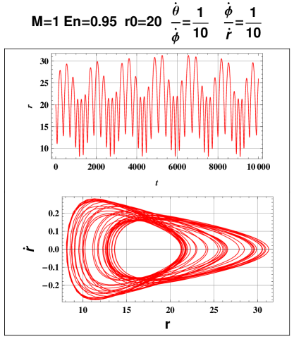
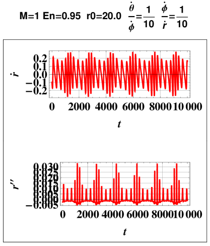
Figure 1: Plots along the panel lines of: $r(t)$ (upper left), phase portrait of $r(t)$ versus $\dot{r}(t)$ (bottom left), $\dot{r}(t)$ (upper right) and $\ddot{r}(t)$ (bottom right) for a star of $1M_{\odot}$. The examples we are showing were obtained solving the system for the following parameters and initial conditions: $\mu\approx 1M_{\odot}$, $E=0.95$,$\phi_{0}=0$, $\theta_{0}=\frac{\pi}{2}$, $\dot{\theta_{0}}=\frac{1}{10}\dot{\phi_{0}}$, $\dot{\phi_{0}}=-\frac{1}{10}\dot{r}_{0}$ and $\dot{r}_{0}=-\frac{1}{100}$ and $r_{0}=20\mu$. The stiffness is evident from the trend of $\dot{r}(t)$ and $\ddot{r}(t)$

2.1 Orbits with gravitomagnetic corrections

In this section we show some examples of orbits. In Fig.2 are plotted some basic orbits with the associated field velocities in false colours. Then in Fig. 3 we show the orbits with gravitomagnetic correction (red-line) and without gravitomagnetic correction (black-line). Finally in the Fig. 4 there is the phase portrait with (red-line) and without (blue-line) gravitomagnetic orbital correction respectively. The example we are showing was obtained solving the system for the following parameters and initial conditions: $\mu\approx 1M_{\odot}$, $E=0.95$, $\phi_{0}=0$, $\theta_{0}=\frac{\pi}{2}$, $\dot{\theta_{0}}=\frac{1}{10}\dot{\phi_{0}}$, $\dot{\phi_{0}}=-\frac{1}{10}\dot{r}_{0}$ and $\dot{r}_{0}=-\frac{1}{10}$ and $r_{0}=20\mu$.

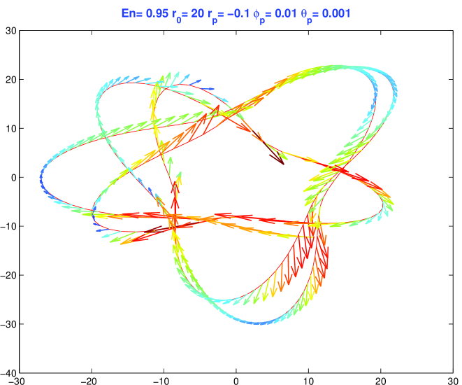
Figure 2: Plots of the basic orbits with the associated field velocities in false colours

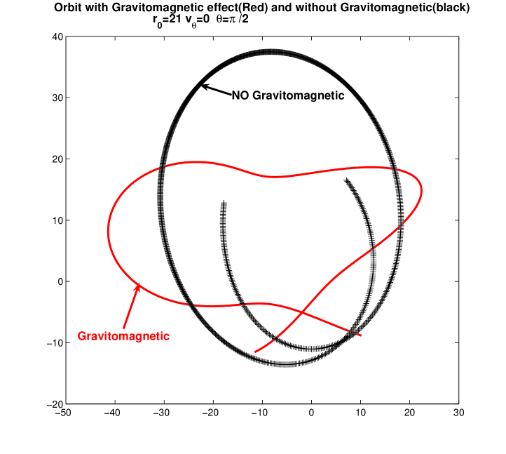
Figure 3: The orbit with gravitomagnetic correction (red-line) and without gravitomagnetic correction (black-line).

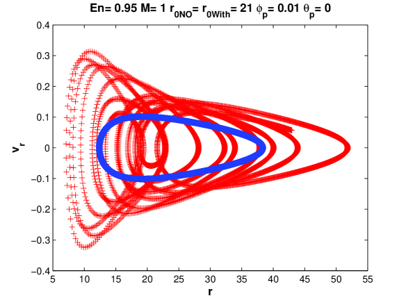
Figure 4: The phase portrait with (red-line) and without (blue-line) gravitomagnetic orbital correction. The example we are showing was obtained solving the system for the following parameters and initial conditions: $\mu\approx 1M_{\odot}$, $E=0.95$,$\phi_{0}=0$, $\theta_{0}=\frac{\pi}{2}$, $\dot{\theta_{0}}=\frac{1}{10}\dot{\phi_{0}}$,$\dot{\phi_{0}}=-\frac{1}{10}\dot{r}_{0}$ and $\dot{r}_{0}=-\frac{1}{10}$ and $r_{0}=20\mu$.

In figure 5 we show some breaking points of the orbital motion with gravitomagnetic corrections.

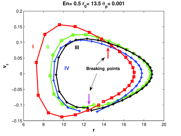
Figure 5: We show the first four orbits in the phase plane: the red one is labelled I, the green is II , the black is III and the blue is IV. As it is possible to see, the orbits in the phase plane are not closed and they do not overlap the orbital closure point; we called these features ’breaking points’.In this dynamical situation, a small perturbation can lead the system to a transition to chaos as prescribed by the Kolmogorov-Arnold-Moser (KAM) theorem.

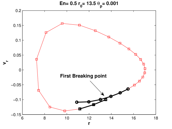
Figure 6: In this figure it is shown the initial orbit with the initial(squares) and final(circles) points marked in black.

3 Gravitational wave in the quadrupole approximation

Now, considering the orbital equations (see S. Capozziello et al. (2009)), we know tha direct signatures of gravitational radiation are its amplitude and its wave-form (C. W. Misner et al., 1973). In other words, the identification of a GW signal is strictly related to the accurate selection of the shape of wave-forms by interferometers or any possible detection tool. Such an achievement could give information on the nature of the GW source, on the propagating medium, and , in principle, on the gravitational theory producing such a radiation. It is well known that the amplitude of GWs can be evaluated by

$$h^{jk}(t,R)=\frac{2G}{Rc^{4}}\ddot{Q}^{jk}~{},$$ (7)

$R$ being the distance between the source and the observer and $\{j,k\}=1,2$, where $Q_{ij}$ is the quadrupole mass tensor

$$Q_{ij}=\sum_{a}m_{a}(3x_{a}^{i}x_{a}^{j}-\delta_{ij}r_{a}^{2})~{}.$$ (8)

Here $G$ is the Newton constant, $r_{a}$ the modulus of the vector radius of the $a-th$ particle and the sum running over all masses $m_{a}$ in the system. At this point we computed the amplitude components with gravitomagnetic corrections in geometrized units (S. Capozziello et al. (2009)). We performed the numerical simulations in two cases: i) a NS of $1.4M_{\odot}$ orbiting around a Super-MBH ( e.g. Sagittarius A* $10^{6}M_{\odot}$) ii) a BH of $10M_{\odot}$ orbiting around a Super-MBH. We considered the reduced mass $\mu=\frac{m_{1}M_{2}}{m_{1}+M_{2}}$. Computations are performed with orbital radii measured in mass units. Initial distances are sampled to show orbits from high eccentricity up to circularity ($e=\frac{r_{max}-r_{min}}{r_{max}+r_{min}}$).

Table 1: Data for GW for a NS of $1.4M_{\odot}$ orbiting around a Super-MBH

$\frac{r_{0}}{\mu}$	$e$	$f(mHz)$	$h$	$h_{+}$	$h_{\times}$
$20$	$0.91$	$7.7\cdot 10^{-2}$	$2.0\cdot 10^{-22}$	$5.1\cdot 10^{-23}$	$5.1\cdot 10^{-22}$
$200$	$0.79$	$1.1\cdot 10^{-1}$	$1.2\cdot 10^{-20}$	$2.2\cdot 10^{-21}$	$3.1\cdot 10^{-20}$
$500$	$0.64$	$1.4\cdot 10^{-1}$	$6.9\cdot 10^{-20}$	$8.7\cdot 10^{-21}$	$1.7\cdot 10^{-19}$
$1000$	$0.44$	$1.9\cdot 10^{-1}$	$2.6\cdot 10^{-19}$	$6.4\cdot 10^{-20}$	$6.4\cdot 10^{-19}$
$1500$	$0.28$	$2.3\cdot 10^{-1}$	$4.8\cdot 10^{-19}$	$3.6\cdot 10^{-20}$	$1.2\cdot 10^{-18}$
$2000$	$0.14$	$2.7\cdot 10^{-1}$	$5.9\cdot 10^{-19}$	$4.9\cdot 10^{-20}$	$1.3\cdot 10^{-18}$
$2500$	$0.01$	$3.1\cdot 10^{-1}$	$5.9\cdot 10^{-19}$	$1.7\cdot 10^{-20}$	$9.2\cdot 10^{-19}$

In Fig. 7-9 we show respectively the field velocities of the orbits along the axes of maximum covariances, the total gravitational emission waveform $h$ and the gravitational waveform polarizations $h_{+}$ and $h_{\times}$ for a NS of $1.4M_{\odot}$. The waveform were computed for the Earth-distance from Sagittarius A (central Galactic Black Hole). We obtained the numerical examples solving the ODE system for the following parameters and initial conditions: $\mu\approx 1.4M_{\odot}$, $E=0.95$,$\phi_{0}=0$, $\theta_{0}=\frac{\pi}{2}$,$\dot{\theta_{0}}=0$, $\dot{\phi_{0}}=-\frac{1}{10}\dot{r}_{0}$ and $\dot{r}_{0}=-\frac{1}{100}$ and $r_{0}=(20\div 1000)\mu$. See also Fig. 7-9 and Table 1.

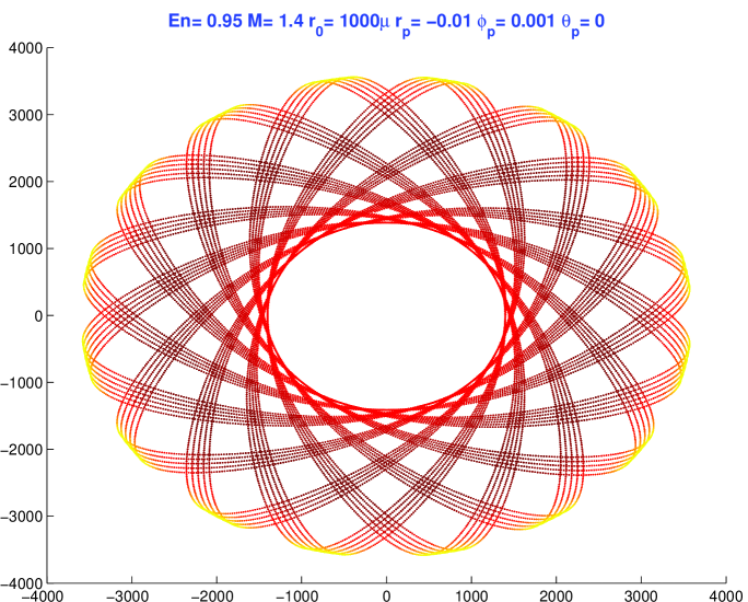
Figure 7: Plot of field velocities of the orbits.

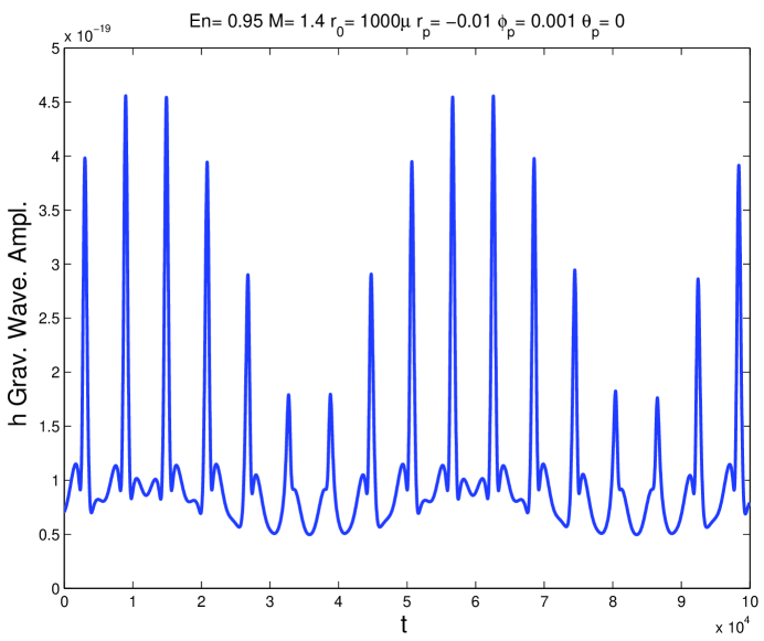
Figure 8: Total gravitational emission waveform $h$ for a neutron star of $1.4M_{\odot}$

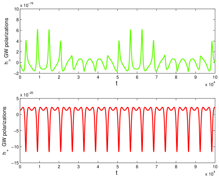
Figure 9: The gravitational waveform polarizations $h_{+}$ and $h_{\times}$ for a neutron star (NS) of $1.4M_{\odot}$

Finally we show in Fig. 10 the plot of the estimated $h$ GW-strain-amplitudes for the considered binary sources at Galactic Center distance. The blue-line is the foreseen LISA sensitivity (one year integration $+$ white dwarf background noise). The red diamonds ($1.4M\odot$ ) and the green circles ( $10M\odot$) are the $h$ values for the systems we have studied.

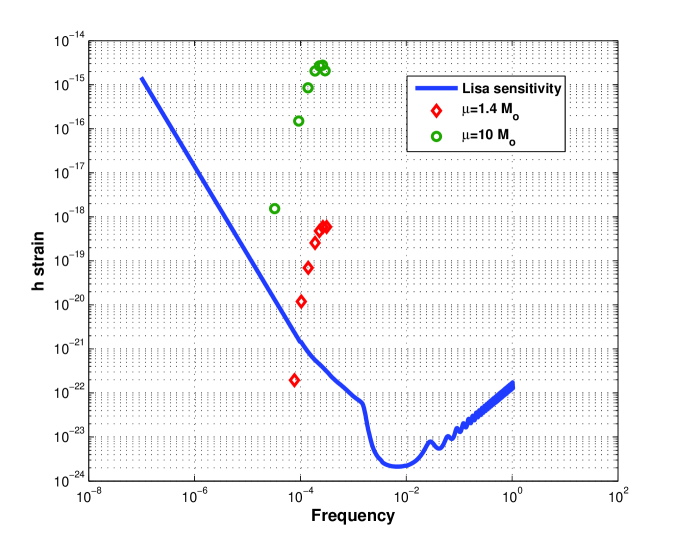
Figure 10: Plot of estimated mean values of gravitational emission in terms of strain $h$ for two binary sources from the galactic center with reduced mass ratio $\mu\approx 1.4M_{\odot}$ (red diamonds) and $\mu\approx 10M_{\odot}$ (green circles). The blue line is the foreseen LISA sensitivity curve. The waveforms were computed for the Earth-distance to Sagittarius A (central Galactic Black Hole).

4 Concluding Remarks

The gravitomagnetic effect could give rise to interesting phenomena in tight binding systems such as binaries of evolved objects (neutron stars or black holes). The effects reveal particularly interesting if v/c is in the range $(10^{-1}\div 10^{-3})c$. They could be important for objects captured and falling toward extremely massive black holes such as those at the Galactic Center. Gravitomagnetic orbital corrections, after long integration time, induce precession and nutation effects capable of affecting the stability basin of the orbits. The global structure of such a basin is extremely sensitive to the initial radial velocities and angular velocities, the initial energy and masses which can determine possible transitions to chaotic behavior. In principle, GW emission could present signatures of gravitomagnetic corrections after suitable integration times in particular for the on going LISA space laser interferometric GW antenna .

References

• A. Einstein (1913) A. Einstein, Phys. Z. 14 (1913) 1261.
• H.Thirring (1918) H. Thirring, Phys. Z. 19 (1918) 204.
• J. Lense and H.Thirring (1918) H. Thirring, Phys. Z. 19 (1918) 33; J. Lense and H. Thirring, Phys. Z. 19 (1918) 156; B. Mashhoon, F.W. Hehl and D.S. Theiss, Gen. Rel. Grav. 16 (1984) 711.
• C. W. Misner et al. (1973) C. W. Misner, K.S. Thorne, J.A. Wheeler, Gravitation, Freeman, New. York (1973).
• S. Capozziello et al. (2001) S. Capozziello, V. Re, Phys. Lett. A 290 (2001) 115.
• S. Capozziello et al. (2009) S. Capozziello, M. De Laurentis, F. Garufi, L. Milano: Physica Scripta vol 79 pg 025901,(2009).
• S. Capozziello et al. (2009) S. Capozziello, M. De Laurentis, L. Forte, F. Garufi, L. Milano, submitted to Physica Scripta, (2009).