Exact Algorithm for Sampling the 2D Ising Spin Glass

Abstract

A sampling algorithm is presented that generates spin glass configurations of the 2D Edwards-Anderson Ising spin glass at finite temperature, with probabilities proportional to their Boltzmann weights. Such an algorithm overcomes the slow dynamics of direct simulation and can be used to study long-range correlation functions and coarse-grained dynamics. The algorithm uses a correspondence between spin configurations on a regular lattice and dimer (edge) coverings of a related graph: Wilson’s algorithm [D. B. Wilson, Proc. 8th Symp. Discrete Algorithms 258, (1997)] for sampling dimer coverings on a planar lattice is adapted to generate samplings for the dimer problem corresponding to both planar and toroidal spin glass samples. This algorithm is recursive: it computes probabilities for spins along a “separator” that divides the sample in half. Given the spins on the separator, sample configurations for the two separated halves are generated by further division and assignment. The algorithm is simplified by using Pfaffian elimination, rather than Gaussian elimination, for sampling dimer configurations. For $n$ spins and given floating point precision, the algorithm has an asymptotic run-time of $O(n^{3/2})$; it is found that the required precision scales as inverse temperature and grows only slowly with system size. Sample applications and benchmarking results are presented for samples of size up to $n=128^{2}$, with fixed and periodic boundary conditions.

I Introduction

Materials with quenched disorder, such as spin glasses, can have extremely long relaxation times, so that laboratory samples exhibit non-equilibrium behavior over many decades in time scale BinderYoung ; YoungBook ; MemoryExpt . Spin glass materials exhibit “aging”, a slow evolution in the magnetic response, for example, and non-equilibrium phenomena such as “rejuvenation”, where changes in the temperature can undo the effects of aging. As these phenomena take place over time scales much longer than the microscopic time scale for individual spins, these effects must be due to the collective behavior of many spins. As analytical work is very difficult in disordered materials FisherHuse ; ParisiRSB , numerical simulations have been important in building a picture of the low-temperature phase of models of disordered spin systems (e.g., KatzgraberYoung ; Rieger ; Cugliandolo ).

Numerical work using direct local Monte Carlo simulation of the dynamics and equilibration JANUS indicate that models such as the Edwards-Anderson model EA possess the long relaxation times that are at least necessary to start to explain these behaviors. Given the direct correspondence between simulation time and “experimental” time, though, the same long relaxation times that one is seeking to understand make such simulations very difficult, even though very long simulation times are used JANUS .

Various alternate approaches and approximations have been developed to address the difficulties of direct simulation. These approaches can be used to determine both the equilibrium state and how this state is approached. When the primary concern is the understanding of the equilibrium state, many studies have sought to find the ground state of given samples, as many of the properties of the low-temperature phase are believed to be given by the properties of the ground state (such as the sample-to-sample fluctuations in the ground state energy or the length-dependent domain wall free energy) HoudayerMartin ; ManyHartmann ; LiersEtal ; PalassiniYoung ; BoettcherEO . This direction of research is based on developing faster exact methods and accurate heuristic methods for finding the spin configuration that minimizes a Hamiltonian with fixed random couplings. The search for a ground state configuration is closely connected with combinatorial optimization methods developed in computer science, though finite-dimensional spin glasses additionally lend themselves to real-space techniques inspired by the renormalization group HoudayerMartin . Equilibrium quantities at finite temperature, such as the partition function and density of states, can be computed for the 2D Ising spin glass. The approach to the ground state and non-equilibrium properties can then be studied by direct simulation or possibly heuristically by real-space blocking of the degrees of freedom PatchworkDynamics .

We present here an algorithm that extends these approaches to allow for exactly sampling the configurations of the disordered Ising model on 2D lattices without the use of Markov Chain Monte Carlo (MCMC). For $n$ spins, this algorithm takes $O(n^{3/2})$ steps and in practice has a running time that grows only somewhat faster, i.e., somewhat more rapidly than $L^{3}$, at fixed temperature. As lower temperatures $T$ require more precise arithmetic, the running time grows roughly as $T^{-1}$. The algorithm is based on Wilson’s algorithm for sampling planar dimer models Wilson . We use a mapping of the Ising spin glass model to the dimer problem for the decoration of the graph dual to the spin lattice Barahona ; KastCities . We take advantage of the regular structure of the square lattice to simplify the algorithm and also modify the matrix algebra of Wilson’s algorithm so that the calculation is both simpler and more numerically stable.

This algorithm for sampling provides an opportunity to study many outstanding questions for 2D spin glasses in much more detail than possible with MCMC computations. For example, the dependence of replica overlaps on temperature and sample size can be directly computed. Correlation functions are easily found: these can be used to study the decay of correlations at finite temperature in both Gaussian and $\pm J$ models, which differ in some aspects at $T=0$. The power law decay of spin-spin correlations are presumed to behave as $r^{-\eta}$ up to the correlation length: how $\eta$ depends on model and is related to thermodynamic quantities such as the heat capacity is still not completely understood correlations .

I.1 Model

The Edwards-Anderson (EA) spin glass model is a prototypical model for disordered materials. The EA spin glass model has the Hamiltonian

$${\mathcal{H}}_{\mathcal{J}}(\mathcal{S}) = -\sum_{\langle ij\rangle}J_{ij}s_{i}s_{j},$$ (1)

where the $\mathcal{J}=\{J_{ij}\}$ are sample-dependent couplings. For example, the $J_{ij}$ can be chosen independently and randomly from a Gaussian distribution or from a bimodal distribution $J_{ij}=\pm 1$ (the $\pm J$ model), with mean zero and variance 1 in either case. These couplings connect two neighboring spins, located at points $i$ and $j$ in the sample. The spins $s_{i}$ are Ising spins, i.e., each $s_{i}=\pm 1$. We will only be able to exactly sample in the 2D case. We will study the square lattice of spins in both the case of periodic boundary conditions, where the bottom row of spins is connected to the top and the left column to the right column, and the case of fixed boundary conditions, where the spins on the boundary of the square sample are fixed. A spin configuration $\{s_{i}\}=S\in\mathcal{S}$ is an assignment of spin values $s_{i}$ to each of $n$ sites $i$; there are $2^{n}$ possible spin configurations in the state space $\mathcal{S}$. A ground state spin configuration $S_{\mathrm{G}S}$ that minimizes the Hamiltonian can be found in polynomial time using a minimum-weight perfect matching algorithm, if the edges $\langle ij\rangle$ which connect nearest neighbor sites and the sites $\{i\}$ form a planar graph Barahona . At positive temperature $T=\beta^{-1}$, the partition function for a given realization of disorder $\mathcal{J}$ is $Z_{\mathcal{J}}=\sum_{S^{\prime}}\exp[-\beta{\mathcal{H}}_{\mathcal{J}}(S^{\prime})]$ and the probability of observing a spin state $S$ in a sample defined by $\mathcal{J}$ is $P_{\mathcal{J}}(S)=Z_{\mathcal{J}}^{-1}\exp[-\beta{\mathcal{H}}_{\mathcal{J}}(S)]$ in equilibrium.

I.2 Exact computation of the partition function

It has long been known that the partition function of the 2D ferromagnetic ($J_{ij}\equiv 1$) Ising model with no external magnetic field can be found exactly by computing the determinant of a matrix derived from the spin lattice. One type of construction of this determinant uses a sum over sets of closed loops on the spin lattice: these loops represent the terms in a high-temperature expansion of the partition function. The first published construction of these type of loops is that of Kac and Ward KacWard , who directly count the polygonal loops. A technique for constructing the relevant matrix for the determinant technique is to map the Ising model onto a dimer covering problem on a decorated lattice $G$ KastCities ; FishCities , where the spins in the original lattice are replaced by a subgraph, a Kasteleyn or Fisher city (a dimer covering is a set of edges in the graph such that every node belongs to exactly one selected edge). The Kasteleyn matrix $K$ of the graph $G$ for the dimer problem describes the connections between neighboring nodes. This square matrix, which is indexed by a numbering of the nodes of $G$, has non-zero entries at locations that are indexed by the two ends of a connection between the nodes. Counting the partition function for dimer coverings is equivalent to computing the Pfaffian of the Kasteleyn matrix, where the Pfaffian in this case is a square root of the determinant. These Pfaffian techniques have been used for the exact solution of the pure Ising model in the thermodynamic limit KacWard ; KastCities ; FishCities and, e.g., for computing the density of states in finite samples. Beale Beale rewrote the Pfaffian in a form that allows for faster direct computation of the partition function in a pure ferromagnetic model. As the derivation of the correspondence between the partition function of the Ising model and the determinant or Pfaffian methods for finite samples does not rely on a homogeneous coupling constant $J_{ij}$, these methods can also be applied to spin glass samples in two dimensions. This correspondence has thus been used to compute directly the partition function (and density of states) for disordered samples SaulKardar ; GLV . Pfaffian techniques can also be used to compute degeneracies and correlation functions in the $\pm J$-model (where couplings are all of the same magnitude, but randomly ferromagnetic or antiferromagnetic between neighboring spins) BlackmanPoulter and has been used to study the heat capacity of this same model at low temperatures (e.g., see LukicEtAl ).

I.3 Review of configuration sampling

Being able to compute the partition function (and often the density of states as a by-product) is useful in computing such quantities as domain wall free energies, sample-to-sample fluctuations in the free energy, specific heat, and other global quantities. By computing the partition function for fixed relative spin configurations, one can also calculate correlation functions BlackmanPoulter . But for many purposes, such as faster computation of correlation functions, the organization of states in a spin glass, or for use in a heuristic for studying the dynamics of disordered materials PatchworkDynamics , it is useful to be able to generate sample configurations, given a realization of the disorder. For sampling the equilibrium behavior of the system, it is sufficient to generate such samples with their proper Boltzmann probability $P_{\mathcal{J}}(\mathcal{S})$. For nonequilibrium dynamics, such sampling can be used in patchwork dynamics, which is closely related to the renormalization approaches to nonlocal dynamics used in multigrid Monte Carlo methods and hierarchical genetic methods HoudayerMartin ; Janke .

Heuristic sampling, where there is no proof of exactness, is typically done using the Markov chain Monte Carlo (MCMC) method. In MCMC methods, local probabilistic dynamics that obey detailed balance are used to update the spins. At long times, the probability of observing a configuration should be the equilibrium probability. The equilibration times using this method can be prohibitively long, though, especially in glassy systems such as the 2D spin glass 2DISGMonteCarlo . Some faster Monte Carlo methods have been developed for the 2D spin glass at low temperature FasterMCAlgs , but with any such method there is also a question of how to test whether equilibrium is achieved with sufficient accuracy. It is of use to have criteria to confirm converges of the Markov chain to the equilibrium distribution. Propp and Wilson ProppWilson proposed a technique for generating exact samples with MCMC by “coupling from the past” (CFTP). In this framework, it is possible to verify that the system has converged from all possible initial conditions to a single state, at which point it is exactly in equilibrium. This approach often makes use of a natural partial ordering of configurations that is used to guarantee convergence. For disordered models, there is often no such obvious partial ordering of the states that ensures convergence of CFTP. Chanal and Krauth ChanalKrauth have nevertheless succeeded in applying CFTP to the Ising spin glass using a coarse-grained organization of the states: at first, all states are possible; as the Markov chain is developed and the number of states is reduced by coupling, the constraint on allowed states is further coarse-grained, until a single whole sample state is left. But the coupling time (time for convergence to a single sample) is still of the order of the equilibration time, which of course can be very long at low temperatures.

Sampling with the exact Boltzmann weights has been implemented and applied to the Migdal-Kadanoff (MK) lattice, which is not a finite-dimensional lattice, but is used to approximately represent finite-dimensional lattices. As the MK lattice has a hierarchical structure, the spin configurations can be summed over successive scales, starting from the smallest, to compute the partition function and the relative partition functions can be used to sample the spins. This was done in Refs. SasakiMartin, and JorgKatzgraber, to study chaos and spin overlap on hierarchical lattices.

Exact sampling of configurations can always be carried out in time polynomial in the size of the sample, if the partition function may be calculated efficiently. One direct, but somewhat slow method, is to assign a single spin at random and then compute the partition function conditioned on assignment of individual neighboring spins; this requires $n=L^{d}$ computations of the partition function for $O(n)$ spins. Such a technique is mentioned as a possibility, for example, in Ref. KrauthBook, . As the partition function can be computed in $O(n^{3/2})$ steps, this would require $O(n^{5/2})$ arithmetical steps. There are other methods for carrying out exact sampling, however.

Exact sampling of ferromagnetic Ising systems (in any dimension) may be performed in polynomial time RandallWilson . This technique works in the Fortuin-Kasteleyn cluster representation and successively removes bonds and spins through a reduction technique. A related problem, sampling configurations of dimer coverings on a planar bipartite lattice, has an elegant sampling technique ProppAD ; ZengEtal , which exactly maps the statistical mechanics on an $L\times L$ lattice to an $(L-1)\times(L-1)$ lattice with modified weights on the edges. Other techniques for calculating the exact partition function of the 2D Ising Spin Glass, such as the Y-$\Delta$ technique of Loh and Carlson LohCarlson , are quite similar in spirit to the dimer covering algorithm. This technique also involves an efficient recursive reduction of any planar graph to a smaller graph, but when frustration is present the intermediate reduced bond strengths can become complex, which complicates possible sampling techniques.

I.4 Overview of algorithm

We now outline the crucial points for our application. In two dimensions, there is a one-to-one correspondence between spin configurations of the Ising model with arbitrary couplings and dimer configurations on a decorated version of the dual lattice. The individual spin and dimer configurations have the same energy, so the corresponding configurations have the same Boltzmann weights $Z^{-1}\exp(-\beta E)$, where $Z$ and $E$ are the partition function and configuration energy for either the dimer or spin problem. We can therefore generate sample spin configurations by sampling among dimer configurations and mapping them to the spin representation. Note that the traditional method for calculating the partition function is a mapping between the primal lattice and a dimer model: a dimer configuration, which defines loops in a high temperature expansion of the partition function, does not directly map onto a unique spin configuration. Using the dual lattice, however, allows for such a map.

Wilson’s algorithm may be used to sample dimer configurations efficiently for any planar lattice, so efficient sampling of the Ising model can be carried out on general planar samples. One requirement for Wilson’s algorithm is an efficient method to recursively subdivide the lattice; this task is straightforward on a regular lattice: we subdivide or separate the sample by choosing two adjacent rows or columns of spins. The spins on these two lines are the separator sites for the spin lattice. These separator spins are then assigned by a sequence of weighted choices. The weights for the choice of these spins are found, in essence, by computing the needed correlators between each pair of spins situated on these two lines. Once the spins on the separator have been chosen and fixed, this division and sampling is repeated on finer and finer spatial scales, using the solved spins as fixed boundary conditions for the subsamples. Besides allowing for recursive assignment of spins on the separators, this nested dissection is used to efficiently organize the needed sparse matrix computations.

We have also simplified the algorithm significantly by using Pfaffian elimination, rather than Gaussian elimination. Pfaffian elimination was used by Galluccio, Loebl, and Vondrak GLV in computing the partition function, but it can also be used to advantage in sampling. We use a sparse matrix representation that greatly reduces the amount of space and time needed: due to the regular nature of the lattice, all of the primitive operations can be explicitly precomputed and then applied to many distinct samples of the same size. We find that the number of relevant matrix elements (out of the full $O(n^{2})$ potential elements) that are “visited” during the computation scales approximately $\sim n$ and that the number of operations obeys the expected growth $\sim n^{3/2}$.

Though the form of the algorithm that we use is based upon and parallels Wilson’s algorithm, we present the method in detail here. We do this in order to review the method itself, emphasize the relationship between matchings and the Ising model, present our form of the matrix algebra that we use for sampling dimer matchings, and describe sampling for non-planar graphs, such as used for periodic boundary conditions.

I.5 Implementation results

As one of the primary motivations for the development of our algorithm is its potential use in patchwork dynamics PatchworkDynamics , we test our algorithm by timing it in this context, random patches of a sample with Gaussian bonds, where the variance of the couplings $J_{ij}$ is unity and the mean coupling $\overline{J_{ij}}=0$. Our code was developed with the possibility of using different data types as the matrix elements in the calculation. Specifically, we test the algorithm using double precision numbers, floating point numbers of arbitrary precision, and with exact rational Boltzmann weights. As the weights in the computation can vary over a large range and a Pfaffian elimination technique is used to cancel out matrix elements, similar to Gaussian elimination, the algorithm can produce unstable results using the floating point types, if proper care is not taken. The likelihood of an instability increases with increasing system size and with lower temperature. In trying to balance the stability and accuracy of the sampling against the running time, we determine the arithmetical precision needed to reliably sample a configuration. Sample results for configurations are displayed in Fig. 1. Details of the precision requirements and example running times are given in Sec. III.5.

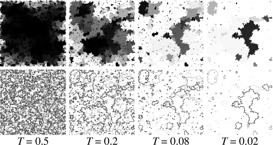
Figure 1: Results of applying the sampling algorithm to an individual 2D Ising spin glass sample, for temperatures $T=0.5,0.2,0.08,0.02$, for a single Gaussian spin glass sample with fixed boundaries. The images show the variability of the spin assignments (top) and of the domain walls (bottom) over a range of temperatures, in a sample with $n=126^{2}$ variable spins surrounded by a layer of fixed spins. At least 240 samples were generated at each temperature. The gray scale values indicate the probability of a given spin being fixed (upper row) or of neighboring spins being fixed relative to each other (lower row). For spin assignments, the darkest colors indicate that the spin is equally likely to be up or down, while light colors indicate that the spin occurs with a single alignment in nearly all sampled configurations. These alignments result from correlations with the fixed boundary spins. For the domain walls displayed in the lower row of images, the lines indicate the probability of relative domain walls between two configurations: the darkest lines indicate the bond dual to that domain wall has a 50% chance of opposite or equal relative orientations; where there is no line separating two spins (or only a very light one), the two spins have a very high probability of a single relative orientation, either aligned or opposite. Specifically, the bond satisfaction variance $\mu_{i,j}(1-\mu_{i,j})$ is plotted along each dual edge, where $\mu_{i,j}$ is the frequency of the $J_{ij}s_{i}s_{j}$ being positive. Note that as $T$ decreases, the frequency of specific droplet excitations, outlined by domain walls, can either increase or decrease, reflecting the sensitivity of the configurations to temperature. This can be seen, for example, in two of the regions that are active at $T=0.02$, the approximately $20\times 20$ region in the far upper left and the approximately $30\times 60$ region at the center right: the spins in the former become more fixed as temperature decreases while the spins in the latter region become more variable (darker) when the temperature is decreased from $T=0.08$ to $T=0.02$.

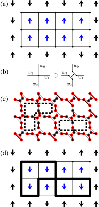
Figure 2: [color online] A depiction of the correspondence between domain wall loops for an Ising spin system and dimer matchings on the decorated dual lattice $G$. (a) A spin system with fixed boundary conditions; an up arrow at location $i$ indicates $s_{i}=+1$ and a down arrow indicates $s_{i}=-1$. The dual lattice $G_{0}$ is indicated by the lines connecting the dual nodes. (b) A Fisher city replacement. Each dual lattice node is expanded to a Fisher city, a set of six nodes composed of two linked triangles, to generate the decorated lattice. For work on the square lattice, the bond strengths are set to be $w(e_{ij})=0$ inside the city, and the bond strengths between the cities, indicated here by the notation $w_{d}$, $d=0,1,2,3$, are set according to Eq. (3). (c) An example dimer covering (i.e., perfect matching) $M$ on the decorated graph $G$. The thicker (also red) bonds with circular ends indicate edges in $M$. The domain walls, composed of dimers that connect distinct cities, are indicated by dashed lines. (d) When the cities are contracted out from $G$, the loops on $G_{0}$ remain. Given this choice of dimer covering $M$, the spins that are inside the domain walls are flipped to create the new sampled configuration.

II Mapping the Ising model to a dimer model

In order to sample Ising spin configurations via the sampling of dimer configurations, one requires a one-to-one correspondence between the Ising spin configurations $\mathcal{S}$ on a given lattice and the dimer covering configurations $\mathcal{M}$ on a related graph $G$. Such mappings have been constructed for application to the more straightforward problem of computing the partition function. These mappings link the problem of computing $Z_{\mathcal{J}}$ to a weighted enumeration of all perfect matchings $\mathcal{M}$ on $G$. A single perfect matching on a graph $G=(V,E)$, where $V$ are vertices (nodes) and $E$ are edges connecting pairs of vertices, is a choice of a subset of edges $M\subset E$, the matching or dimer covering, such that every vertex belongs to exactly one edge in $M$ (see Fig. 2). The generally established procedure for constructing a mapping between spin configurations and perfect matchings is to identify closed loops on some relevant graph, $G_{0}$, where $G_{0}$ is either the primary grid (the spin lattice) or the dual lattice (the lattice of plaquettes). The partition function, originally a sum over spin configurations, can be represented as a weighted sum over choices of loops in $G_{0}$. This summation over loops can be carried out by summing over matchings on a graph $G$, constructed by replacing the nodes of $G_{0}$ with either Kasteleyn or Fisher “cities” KastCities ; FishCities , subgraphs constructed of a few nodes and edges. Perfect matchings on this decorated lattice $G$ then have the property that an even number of the covered edges are incident upon any given city. The edges of a matching $M$ that connect cities are therefore even at each city; contracting the cities back to single points then gives the city-connecting dimers that compose the loops in $G_{0}$ (see Fig. 2).

One mapping between spin configurations and sets of loops is based on a high temperature expansion of the partition function of the Ising model, where $G_{0}$ is the spin lattice and the loops, composed of bonds connecting nearest-neighbor spins, represent individual terms in the expansion of $Z_{\mathcal{J}}$ in powers of $\exp(-\beta J_{ij})$. The direct replacement of each Ising spin with a “city” gives representation of loops by a dimer matching KastCities ; FishCities ; GLV . The weight of dimer configurations can then be summed using Pfaffian methods KastCities giving, for example, the Kasteleyn solution of the Ising model. However, there is no direct correspondence between individual sets of loops and spin configurations.

Alternately, a mapping to $G$ can be defined by taking $G_{0}$ to be the dual lattice Barahona ; GSKastCities . This mapping, in contrast with the approach of decorating the original lattice, allows for direct sampling of Ising spin configurations. The loops on the dual graph represent a loop expansion in terms of domain walls. The expansion in domain walls, if expressed relative to the ground state, would be a low-temperature expansion. More generally, the summation is over relative domain walls between a reference configuration and any other configuration. A direct correspondence between spin configurations and dimer configurations therefore exists as domain walls uniquely define a spin configuration, given a reference configuration, up to the possibility of a global spin-flip symmetry.

Let $R=\{r_{i}\}$ be a reference configuration of Ising spins $r_{i}=\pm 1$. We emphasize that this choice is completely arbitrary: it need not be a ground state. For convenience $R$ can be a configuration with all spins up or a previously sampled configuration. For a given sampling $S$ of the spin configuration, $S=\{s_{i}\}$, the loops of dual edges that separate spins $i$ and $j$ with $r_{i}s_{i}\neq r_{j}s_{j}$ define the relative domain walls between $R$ and $S$. (For the ferromagnetic Ising model, one usually takes $r_{i}\equiv 1$, so that the domain walls separate regions where $s_{i}=1$ from regions where $s_{i}=-1$.)

In this reference configuration, for each pair $i,j$, define $R_{ij}=r_{i}r_{j}$ as the reference satisfaction of bond $i,j$. Then, for this fixed $R_{ij}$, we can simply rewrite the Hamiltonian as

$$\mathcal{H_{J}}(S) = -\sum_{\langle ij\rangle}J_{ij}\left(s_{i}s_{j}-R_{ij}+R_{ij}\right)$$ (2)

$$= \mathcal{H}_{R}+\mathcal{H}_{G}\,,$$

with $\mathcal{H}_{R}=-\sum_{\langle ij\rangle}J_{ij}R_{ij}$, the energy of the reference configuration and $\mathcal{H}_{G}=-\sum_{\langle ij\rangle}J_{ij}\left(s_{i}s_{j}-R_{ij}\right)$, which will be rewritten as the Hamiltonian of the corresponding dimer model is the energy of the domain walls between the configurations $R$ and $S$. Note that $\mathcal{H}_{R}$ is the same for all spin configurations, but must be tracked if comparing the effects of changing boundary conditions or comparing with ground state energies, for example.

Let the decorated graph $G=(V,E)$ have the vertex set $V$, which has size $|V|=2N$, $N$ being the number of dimers in a perfect matching of the vertices, and the edge set $E=\{e_{qr}\}$ where each edge connects two nodes, $e_{qr}=(q,r)$, for some $q,r\in V$. Then, given a set of relative domain wall loops, the dimer configuration is uniquely defined by selecting dimers that connect cities and cross bonds $J_{ij}$ where $s_{i}s_{j}\neq R_{ij}$, i.e., that overlie the domain walls in $G_{0}$, and the subsequent unique choice of matching for dimers internal to the cities. Choosing an energy function $w(e)$ for edges in $E$ with $w(e_{qr})=0$ for bonds in the cities and

$$w(e)=2J_{ij}R_{ij}$$ (3)

for dual edges $e$ crossing bonds between spins $i$ and $j$ gives

$$\mathcal{H}_{G}(M) = \sum_{e\in M}w(e)$$ (4)

as a consistent energy function for matching configurations in $M$. The Ising model and matching model can therefore be made equivalent, up to a global energy shift $\mathcal{H}_{R}$.

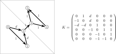
Figure 3: The node indexing and edge orientations within a Fisher city (left) and the corresponding elements of the $6\times 6$ submatrix of the Kasteleyn matrix $K$ (right). The numbering of nodes is shown for the first city listed in the dual lattice; subsequent cities have multiples of 6 added to their indices. In the case of the square spin lattice (indicated by the outer square bonds on the original spin lattice), all non-zero $K$ elements, including $d$, are set to unit magnitude. The labeling of the $0\rightarrow 2$ and $1\rightarrow 2$ edges indicate how the strengths can be modified in the case of the triangular lattice: in this case, one can set $d=\exp[-\beta w(e_{d})]$ to account for the diagonal bond $e_{d}$ perpendicular to the $2\rightarrow 3$ edge. The Kasteleyn matrix has row $a$ and column $b$ indices $a,b=0,\ldots,5$.

Because each dimer configuration corresponds to a spin configuration with the same energy, picking a sample from the dimer model with the correct probability directly produces a corresponding spin configuration that has the same probability of occurring. We chose to use Fisher cities for this work, instead of Kasteleyn cities KastCities , as they are simpler to sample using Wilson’s algorithm on a square lattice. Also, by modifying the weights of the Fisher cities, we can also very easily change the weights to simulate triangular lattices (see Fig. 3).

II.1 Matchings and the Kasteleyn Matrix

Given the mapping between matchings using dual lattice cities and spin configurations, we now briefly review the correspondence between dimer matchings and Pfaffians. Extensive discussion and examples can be found in, for example, Refs. KastCities ; Robertson ; KrauthBook . As a mathematical object, the Pfaffian $\operatorname{Pf}(A)$ can be defined for general $2N\times 2N$ antisymmetric square matrices $A=\{a_{qr}|q,r=0,\ldots,2N-1\}$, $a_{qr}=-a_{rq}$ by a restricted sum over permutations $P=p(t)$ of the indices $t=0,1,\ldots,2N-1$,

$$\operatorname{Pf}(A)=\sum_{P\,\mathrm{ordered}}(-1)^{\sigma(P)}a_{q_{1}r_{1}}a_{q_{2}r_{2}}\ldots a_{q_{N}r_{N}}\ ,$$ (5)

where $\sigma(P)$ is the sign of the permutation from the sequence $0,\ldots,2N-1$ to the sequence $q_{1},r_{1},\ldots,q_{N},r_{N}$ and the restriction to ordered $P$ is to rearrangements where $q_{k}<r_{k}$, for all $1\leq k\leq N$, and $q_{1}<q_{2}<\ldots<q_{N}$. We also have that $[\operatorname{Pf}(A)]^{2}=\mathrm{det}(A)$.

It turns out that summing over permutations with these two restrictions is exactly the way to sum over dimer coverings for a planar graph $G$, if the matrix elements of $A$ are chosen properly. A matrix whose Pfaffian is $Z_{\mathcal{M}}=\sum_{M\in\mathcal{M}}\exp[-\beta\mathcal{H}_{G}(M)]$ is the Kasteleyn matrix $K$. This matrix has entries $K(q,r)$, with $q,r=0\ldots,2N-1$, satisfying $|K(q,r)|=x_{q,r}$, where $x_{q,r}=\exp\{-\beta w[e(q,r)]\}$, and $w[e(q,r)]$ is the bond strength associated with edge $e(q,r)$. Directions for the edges are then chosen so that all loops in $G$ which enclose an even number of nodes include an odd number of counterclockwise edges KastCities . The matrix entry $K(q,r)$ is set to be $x_{q,r}$ if an edge is oriented from $q$ to $r$, otherwise it is set to be $-x_{q,r}$. This convention ensures that each valid dimer configuration has positive net weight. The Kasteleyn matrix is thus a weighted version of a directed adjacency matrix. Using these conventions and weight assignments gives KastCities

$$\operatorname{Pf}(K)=\sum_{M\in\mathcal{M}}\prod_{e\in M}x_{e}=Z_{\mathcal{M}}=Z^{-1}_{R}Z_{\mathcal{J}}\,.$$ (6)

When decorating $G_{0}$ with cities to create $G$, the edges internal to the cities must be assigned orientations. An example of a Fisher city with the correct directionality and the corresponding submatrix is shown in Fig. 3. The orientation of the connections between the cities are from the 4-node in one Fisher city to the 0-node in the city to the right and from the 5-node a city to the 1-node in the city in the row above. To simplify notation for the rest of the paper, we will use $Z$ to indicate $Z_{G}$.

Established analytical and numerical techniques can be used to compute $\operatorname{Pf}(K)=Z$. As these numerical techniques require a number of mathematical operations polynomial in the size of the lattice, specifically growing as $\sim n^{3/2}$, the thermodynamic properties can be efficiently computed. The number of bits needed for exact computations grows with $n$, so that computing, for example, the exact partition function, written out as a polynomial in $\exp(-\beta)$ of a spin glass sample for the $\pm J$ model, where $J_{ij}=\pm 1$, requires $O(n^{7/2})$ primitive fixed-word-length operations GLV .

We extend this correspondence to carry out sampling of spin configurations by applying Wilson’s algorithm. Partial diagonalization of the Kasteleyn matrix generates correlation functions for the choice of the dimers in the matching representation. These correlations are between dimers on a separator of the sample, which divides the sample into two nearly equal places. These correlations functions include the probability of choosing any dimer in a matching, so it is straightforward to determine whether a single dimer is selected in a random matching. The insight developed by Wilson was to update these correlations as dimers are chosen: the effects of partial assignment are propagated inductively to correlations between other dimers, allowing many dimers to be assigned without another factorization of the full Kasteleyn matrix. Once the dimers have been selected on a separator, the two pieces are then solved recursively, using their own separators.

III Wilson’s algorithm

In this section, we describe our implementation of Wilson’s algorithm, as applied and adapted to sampling configurations of the Ising spin glass. Wilson’s algorithm samples dimer coverings: we map the Ising problem to the dimer sampling problem using the mapping described for the dual lattice in Sec. II. Wilson’s algorithm uses a “nested dissection” LRTDissection , i.e., a recursive subdivision of the sample, where each subdivision of $n$ spins is into two pieces of similar size separated by a line of vertices of size $O(\sqrt{n})$, for efficiency. Such a nested dissection was used by Galluccio, Loebl, and Vondrak GLV , to compute the full expansion of the partition function of the $\pm J$ spin glass as a polynomial in $\exp(-\beta)$, using the high temperature expansion formulation of the partition function. This dissection can be phrased using either a dimer description, based on a matching of the decorated graph on the dual lattice, or using spins. The algorithm is necessarily implemented in terms of the former language, but for clarity, it is also convenient to describe it using the latter language, i.e., based on the spins on the original lattice.

Consider a subsample $U$ of Ising spins $\{s_{i}|i\in U\}$, possibly with external fields at the boundary (corresponding to fixed spins bordering $U$; this graph is still planar). To divide this sample into two independent samples, $U^{\prime}$ and $U^{\prime\prime}$, a set $D$ of spins is chosen as a spin separator, so that

$$U=U^{\prime}\cup D\cup U^{\prime\prime}$$ (7)

and no bonds connect spins in $U^{\prime}$ to spins in $U^{\prime\prime}$. We choose this spin separator to be composed of two parallel lines of spins, so that a line of nodes in the dual lattice is contained between the two lines of spins.

It turns out that Wilson’s approach provides an efficient way to assign spin values along this separator, such that the spins are selected with the correct probabilities. That is, let such a spin assignment on $D$ be $S_{D}=\{s_{k}=\pm 1|k\in D\}$. The spin at site $i$ for a choice $S_{D}$ is also written as $S_{D}(i)$. One requires that the probability that the algorithm will generate a particular choice $S_{D}$ is just equal to the probability $P_{\mathcal{J}}(S|S_{D})$ that the properly weighted choice of all spins will yield that particular assignment of spins on the separator $D$, i.e., that

$$P(S_{D})=[Z(U)]^{-1}\sum_{S_{U}|S_{U}(i)=S_{D}(i),\forall i\in D}\exp[-\beta{\mathcal{H}}(S_{U})]\,,$$ (8)

with $S_{U}$ being a particular configuration of the spins in $U$, the sum indexing all possible spin assignments consistent with the choice $S_{D}$, and with $Z(U)=\sum_{S_{U}}\exp[-\beta{\mathcal{H}}(S_{U})]$ the partition function for $U$. The remarkable property of the algorithm to make such a selection implies that this procedure may then be repeated on the remaining unassigned subsystems $U^{\prime}$ and $U^{\prime\prime}$ independently of one another.

We can select the assignment for the spins in $D$ by sampling from the dimer assignments for all the nodes in $\Delta$, where $\Delta$ is the set of all nodes in $G$ that lie inside of $D$ and the connecting edges contained within $D$. This set of nodes $\Delta$ is what is referred to as the separator in Wilson’s work on an algorithm for random dimer assignments.

In order to outline of our version of the algorithm for assigning matchings in $\Delta$, one needs the notion of Pfaffian elimination GLV . Let $K$ be a $2N\times 2N$ skew-symmetric matrix, i.e., $K(q,r)=-K(r,q)$ for $0\leq q,r<2n-1$. A cross operation between $q$ and $j$ is the addition of a multiple of row $q$ to row $r$ and the same multiple of column $q$ to column $r$. If this multiple is given by the factor $\alpha$, the cross operation on $K$ can be written as

$$K\rightarrow L(\alpha,q,r)KL^{T}(\alpha,q,r)\,,$$ (9)

where $L(\alpha,q,r)$ is the lower triangular matrix $I+\alpha\delta_{q,r}$. The matrix $\delta_{q,r}$ has all entries zero except for a unit entry in row $q$ and column $r$. It turns out that the value of $\operatorname{Pf}(K)$ is unchanged by cross operations, as $L$ has unit determinant and $\operatorname{Pf}(BKB^{T})=\det(B)\operatorname{Pf}(K)$ for general $B$ ElectronsMonteCarlo . Pfaffian elimination is the application of multiple cross operations to simplify the matrix. This factorization via Pfaffian elimination has the goal of making the Pfaffian trivial to compute; the simplest form of a skew-symmetric matrix has non-zero values only in the even row superdiagonal elements,

$$Y=\sum_{\ell=0}^{N-1}y_{\ell}\sigma_{2}^{(\ell)}\,,$$ (10)

where $\sigma_{2}^{(\ell)}$ is just the matrix that is non-zero except for the $(2\ell,2\ell+1)$’st entry, which is set to $1$, and the $(2\ell+1,2\ell)$’st entry, which is set to $-1$. In Pfaffian elimination, then, the $\nu$ factors $\alpha_{m}$ and the cross operation locations $q_{m}$, $r_{m}$ are all chosen sequentially so that

$$Y=LKL^{T}\,,$$ (11)

with $L=\prod_{m=1}^{\nu}L(\alpha_{m},q_{m},r_{m})$ and $Y$ is of the form in Eq. (10). The needed choices of $\alpha_{m}$, $q_{m}$, and $r_{m}$ are discussed in more detail in Sec. III.2.

As the factorization of $K$ given by Pfaffian elimination leaves the Pfaffian invariant

$$\operatorname{Pf}(Y)=\operatorname{Pf}(LKL^{T})=\det(L)\operatorname{Pf}(K)=\operatorname{Pf}(K)\ ,$$ (12)

the Pfaffian of the Kasteleyn matrix, and hence the partition function, can be directly found by multiplying the even superdiagonal entries of $Y$.

This elimination procedure resembles the application of Gaussian elimination to compute the $LU$ factorization of a matrix $A$, with $A=LU$ where $L$ is lower triangular with unit elements on the diagonal and $U$ is upper triangular. The product of the diagonal elements of $U$ gives $\det(A)$; here $\operatorname{Pf}(K)$ is the product of the even row superdiagonal elements of $Y$. Factorization via Pfaffian elimination maintains the skew symmetry of the partially factorized $\prod_{m}L(\alpha_{m},q_{m},r_{m})\,K\prod_{n}L^{T}(\alpha_{n},q_{n},r_{n})$ at each stage. Wilson presented his sampling algorithm using Gaussian elimination; we find that Pfaffian elimination both clarifies the algorithm and makes the programming of the algorithm more direct. A version of the algorithm that we implemented using Gaussian elimination was much less stable numerically than the one implemented using Pfaffian elimination.

The factorization of $K$ given by Pfaffian elimination allows the inverse of $K$ to be quickly computed. It is clear from Eq. (12) that

$$K^{-1}=L^{T}Y^{-1}L\ ,$$ (13)

where, given the simple form of $Y$, the inverse of $Y$ is easily found:

$$Y^{-1}=-\sum_{\ell=0}^{N-1}\frac{1}{y_{\ell}}\cdot\sigma_{2}^{(\ell)}\ .$$ (14)

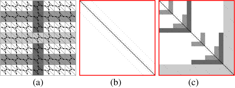
Figure 4: [color online] An example of the nested dissection and the Kasteleyn matrix $K$ for a $6\times 6$ spin lattice sample surrounded by an outer layer of fixed spins. (a) The set of $8\times 8$ Ising spins sit on the sites of the light gray lattice of bonds of strength $J_{ij}$, where the diagonal bonds are indicated for the case of a triangular lattice. The graph $G$ on which the dimer sampling is computed is shown by the darker lines and circular nodes. The gray bands indicate the nested dissection used for these nodes: the lighter gray region contains the dimer separator $\Delta\subset G$ and is bordered by the middle two rows of spins, the spin separator $D$. The darker and medium bands indicate, in order, the subsequent subdivisions of the sample. (b) A display of the non-zero elements of the Kasteleyn matrix $K$, for a left-to-right and top-down ordering of the Kasteleyn cities. The nonzero elements of the $294\times 294$ Kasteleyn matrix for this are shown as black dots. The edges internal to the Kasteleyn cities are closest to the diagonal: further non-zero elements represent connections between the cities. (c) The permuted matrix $K$, where the cities are indexed according to a nested dissection. The gray regions in $K$ include connections contained within each of the separators of the nested dissection, with the same shades as in (a), and between the separators and other nodes. The procedure of Pfaffian elimination can at most affect elements within the gray regions and also the values near the diagonal, for the nodes not contained in the gray regions in (a). Spin values are assigned to $D$ by examining the part of $K^{-1}$ indexed by the nodes of $\Delta$, i.e., the lower right square submatrix contained within the light gray region.

When the matrix $K$ is created, the indexing of the nodes in $G$ is chosen according to a nested dissection of the graph $G$ that maintains the grouping of the Kasteleyn cities. This ordering reduces the amount of work needed to carry out the Pfaffian elimination and is chosen so that the elements of the separator at each level of the dissection are in a block at the lower right part of the submatrix organized by that separator. An example of this ordering, given by the nested dissection, is shown in Fig. 4.

The core of the dimer assignment procedure is based on the relationship between restricted partition functions and the Pfaffian of submatrices of the Kasteleyn matrix. Consider two partition functions, the entire partition function $Z=\operatorname{Pf}(K)$ and the restricted partition function $Z_{p}$, which is sum of weights $\prod_{e\in{G\setminus p}}x(e)$ restricted to matchings that include the fixed partial matching $p=\{q_{1},r_{1},\ldots,q_{k},r_{k}\}$, with matched edges $(q_{1},r_{1}),\ldots,(q_{k},r_{k})$. A listing of the terms that contribute to $Z_{p}$ can be found by removing all nodes in $p$ from the graph $G$ and computing the Pfaffian of $K_{p}$, the Kasteleyn matrix for $G\setminus p$. To find $Z_{p}$, the weights $x$ of the removed edges must then be included, giving

$$Z_{p}=\operatorname{Pf}(K_{p})\prod_{e\in p}x(e)\ .$$ (15)

The weights $x(e)$ are uniform in Wilson’s description, though he noted the possibility of variable weights. The probability $P(p)$ of choosing the edge set $p$ is therefore

$$P(p)=\frac{Z_{p}}{Z}=\frac{\operatorname{Pf}(K_{p})\prod_{e\in p}x(e)}{\operatorname{Pf}(K)}\ .$$ (16)

Given that one has already chosen an edge set $p$ that partially covers a graph, the conditional probability $P(p,u\,|\,p)$ of edge $u$ being in a complete matching that includes $p$ is

$$P(p,u\,|\,p)=\frac{Z_{p,u}}{Z_{p}}=\frac{Z_{p,u}\cdot\operatorname{Pf}(K)}{Z_{p}\cdot\operatorname{Pf}(K)}=\frac{\operatorname{Pf}(K_{p,u})x(u)}{\operatorname{Pf}(K_{p})}\ .$$ (17)

Fundamental relations between determinants and inverse matrices are used in Wilson’s algorithm to speed up the computation of $K_{p}$: we directly adapt these relations for Pfaffian factorization. Let $A$ be a $2m\times 2m$ skew-symmetric matrix, and $0\leq\ell<2m$ be an even integer, and $p=\{t_{1},t_{2},\ldots,t_{\ell}\}$ be a subset of indices for the rows (columns) of $A$. We will use the notation that $A_{p}=A_{t_{1},t_{2},\ldots,t_{\ell}}$ denotes the $(2m-\ell)\times(2m-\ell)$ skew-symmetric matrix given by removing from $A$ all rows and columns with indices in the set $(i_{1},\ldots,i_{\ell})$. The notation $[A]_{t_{1},\ldots,t_{\ell}}$ will denote the $\ell\times\ell$ matrix resulting instead from keeping just those rows and columns and eliminating the rest of the matrix. Using this notation, and the result that $\det(A)=[\operatorname{Pf}(A)]^{2}$, Jacobi’s theorem (or directly using the definition of the Pfaffian to show that element $i,j$ of $A^{-1}$ is $(-1)^{i+j}\operatorname{Pf}(A_{i,j})/\operatorname{Pf}(A)$) implies that Jacobi2

$$\frac{\operatorname{Pf}(A_{i_{1},\ldots,i_{\ell}})}{\operatorname{Pf}(A)}=\pm\operatorname{Pf}([A^{-1}]_{i_{1},\ldots,i_{\ell}})\,,$$ (18)

where the sign depends only on the choice of the indices $i_{1},\ldots,i_{\ell}$.

Eqs. (17) and (18) thus allow one to compute the probability of matching $(q_{1},r_{1}),\ldots,(q_{k},r_{k})$, using the Pfaffian of the inverse of the Kasteleyn matrix where the same rows and columns kept. The Pfaffian factorization of this latter matrix, $\left[K^{-1}\right]_{q_{1},r_{1},\ldots,q_{k},r_{k}}$, can be updated incrementally as successive choices of matched edges are made. This update allows for the progressive computation of the probabilities $P(p,u\,|\,p)=x(u)z_{k}(u)$, where the updated factorization directly gives the value $z_{k}(u)=\operatorname{Pf}\left(\left[K^{-1}\right]_{p,u}\right)/\operatorname{Pf}\left(\left[K^{-1}\right]_{p}\right)$.

Our adaptation of Wilson’s algorithm can now be summarized in outline form:

1. First, order the points of the decorated dual lattice $G$ in a manner consistent with the nested dissection. The elements of the first dual separator $\Delta$ are at the end of this ordering.

2. Using this ordering, set the values of the Kasteleyn matrix $K$, which is stored as a sparse matrix.

3. Factorize $K$ using Pfaffian elimination. We use a pre-computed list of elementary operations to carry out the cross operations for all elements that are potentially non-zero. (Stop here if only the partition function for $U$ is needed; the partition function $Z$ is just the product of alternate superdiagonal elements in $Y$, i.e., $Z=\prod_{\ell=0}^{N-1}y_{\ell}$.)

4. Using this factorization, compute the elements of $K^{-1}$ that are indexed by elements of $\Delta$; this is $[K^{-1}]_{\Delta}$, the lower-right submatrix of $K^{-1}$ with indices contained in $\Delta$. (For some speed up, as suggested in Ref. Wilson, , we only compute the elements of $\left[K^{-1}\right]_{\Delta}$ that are needed in the following steps, at the time those elements are required.)

5. Assign dimers $(q_{1},r_{1}),(q_{2},r_{2}),\ldots$ along the separator $\Delta$:

   1. Choose a node $q_{1}\in\Delta$ such all edges that are incident upon $q_{1}$ are fully contained in $\Delta$. Choose among the potential edges $(q_{1},r_{1})=e$ with the probabilities $K(q_{1},r_{1})\operatorname{Pf}({K}_{q_{1},r_{1}})/\operatorname{Pf}(K)=K(q_{1},r_{1})\operatorname{Pf}([K^{-1}]_{q_{1},r_{1}})$.

   2. Repeat this last substep, 5a, proceeding along the dimer and updating $[K^{-1}]_{q_{1},r_{1},\ldots,q_{k},r_{k}}$ and its factorization, until no more matchings can be added wholly within the set $\Delta$.

6. Use the dimer matching for $\Delta$ to assign spin values in the spin separator $D$, which surround the dimer separator $\Delta$.

7. Recursively repeat items 1-7 for the subproblems $U^{\prime}$ and $U^{\prime\prime}$.

Note that, in some cases, an alteration of this procedure can be used to speed up this method. It might be that faster results can be obtained using simple floating point numbers (double precision), rather than multi-precision numbers, though they may not provide numerical accuracy to carry out all of the calculation. A compromise would be to carry out the computation for only part of the separator at a time, making the computation more stable. The whole matrix $K$ with the remaining unchosen nodes is recomputed and the process is repeated. This method is asymptotically slower, but practical for systems of intermediate size at intermediate temperature.

III.1 Entries of $K$: nested dissection and storage

The Kasteleyn matrix $K$, as defined in Section II.1, is indexed by the nodes of the decorated dual graph $G$. As the entries $K(q,r)=\pm x(q,r)$ of $K$ are non-zero only for entries indexed by neighboring points $q$ and $r$ on the decorated dual lattice, this $O(n)\times O(n)$ matrix has only $O(n)$ non-zero entries. If the nodes are indexed in a natural, geometric, lattice order, the Kasteleyn matrix $K$ is simple, as shown in Fig. 4(b). However, matrix manipulations, such as Pfaffian elimination, for general matrices might lead to the computation of $O(n^{2})$ non-zero entries.

To compute the correlations between spins on the separator, the nodes are reordered, though kept together in city groups. In this reordering, the nodes are each assigned a new index. This reordering satisfies the nested dissection property that, at each level, the separator nodes in $\Delta$, which give the spin sub-sample $U$, have the highest index. This implies that the non-zero values defined by the weights contained within the separator $\Delta$ are at the lower and rightmost parts of $K$, at each level, while the non-zero values for nodes belonging to $U^{\prime}$ and $U^{\prime\prime}$ [see Eq. (7)] are confined to square blocks about the diagonal. An example of the distribution of matrix entries, given this ordering of the nodes $V$ of $G$, is shown in Fig. 4(c). This organization confines all matrix manipulation to a portion of the shaded regions of the matrix and to a narrow band around the diagonal, as unshaded entries away from the diagonal always have value zero. The shaded regions make up $O(N^{3/2})$ entries, though only a subset of even those entries, growing with $N$ approximately as $\sim N$, possibly with a logarithmic correction, are used in the Pfaffian elimination.

Given our specific choice of separator, the nodes of $G$ corresponding to the Kasteleyn cities always form subsequences in the ordering of the nodes. That is, they remain grouped together. Note that the submatrices for each city are uniform in structure. This choice of separator $\Delta$ (as all of the dual nodes between two rows or columns of spins) is not the most efficient, as slightly smaller separators $\Delta\subset G$ can be chosen, but it is a very convenient choice that maintains a uniform structure.

We use this ordering to construct $K$ as a sparse matrix, using $O(N)$ operations and time. The sparse matrix storage scheme is relatively direct (see, e.g. SparseMatrixRef for a discussion on sparse matrix algorithms and storage techniques). We have the advantage here that, for the Pfaffian elimination, both the locations of the needed elements and the list of operations using these elements can be pre-computed and stored on disk. This allows us to place the elements of the matrix $K$ in a linear array with $O(N)$ elements, with the elements ordered by the step at which they are first needed in the Pfaffian elimination. This precomputation is independent of both the data type that we use and the bond strengths for the spin lattice.

III.2 Pfaffian factorization

Figure 5: Example of cross operations used for Pfaffian elimination. (i) A skew-symmetric matrix $K$. (ii) The result of a cross operation $K\rightarrow L(\alpha,i,j)KL^{T}(\alpha,q,r)$ of the first type, with $q=0$, $r=2$, $\alpha=-a$, applied to $K$. This is found by adding $\alpha=-K(q,r)/K(q,q+1)$ times column $q+1$ to column $r$ and then $\alpha$ times row $q+1$ to row $r$, to eliminate the element at location $(q,r)$. (iii) The result of the next cross operation, with $q=0$, $r=3$, and $\alpha=-b$. (iv) The result of two subsequent operations of the second type, where $\alpha(q,r)=-K(q,r)/K(q,q-1)$, for $q=1$, $r=2$ and $q=1$, $r=3$. These latter types of operation are not needed to compute $\operatorname{Pf}(K)$, but are needed for finding $[K^{-1}]_{\Delta}$. The Pfaffian of $K$ is the product of the superdiagonal elements in even rows: here, $\operatorname{Pf}(K)=(1)(1-ac+b)$.

Pfaffian elimination and the concomitant factorization of $K$ proceed by the elimination of elements by cross operations. There are two types of cross operations that are carried out. The first type of operation eliminates all but the first of the non-zero entries in an even row. This is done for an even row $q$ by using (see Eq. 9) $\alpha(q,r)=-K(q,r)/K(q,q+1)$ for all $r\geq q+2$. The second type eliminates all entries in odd rows. This is done for odd $i$ using $\alpha(q,r)=-K(q,r)/K(q-1,q)$ with $r\geq q$. Examples of operations of each type are traced out in Fig. 5.

We note that in carrying out Pfaffian elimination, a potential danger would be that one of the even-row superdiagonal elements, $K(q,q+1)$ with $q$ even, is zero. In this situation, it would be necessary to do a pivoting operation, which would destroy the nested dissection. However, given that the Kasteleyn cities remain grouped together, the sequential pairing of nodes $(0,1),(2,3),\ldots$ is always a matching. Hence the Pfaffian of any upper left portion of the Kasteleyn matrix, as we have arranged it, is non-zero, as the Pfaffian counts matchings (in a weighted fashion), and there is always a matching for the upper left portion of the matrix of unit weight. This implies that all superdiagonal elements in the even rows must be non-zero. This provides a “built-in” version of the permutation of nodes to accommodate a matching that is given in Wilson’s paper Wilson . In the periodic case (Sec. IV), for certain boundary weight choices at $\beta=0$ ($T=\infty$), when the bond strengths have uniform magnitude, there can be “accidental” cancellations which will cause this procedure to fail, as the signed weight of a sub-matching can be exactly zero, even though the Pfaffian is non-zero. In this case, permutation of the remaining elements of the matrix (i.e., “pivoting”) would be needed to remove a zero from the superdiagonal and obtain the correct factorization.

The factorization found by Pfaffian elimination, Eq. (12), then allows for the easy computation of the partition function for the given sample, at the temperature used to set the elements of $K$, if desired. The Pfaffian of the original Kasteleyn matrix is simply the product of the even superdiagonal elements of $Y$,

$$\operatorname{Pf}(K)=\prod_{\ell=0}^{N-1}y_{\ell}\ .$$ (19)

Note that this is the procedure, computation of the Pfaffian of $K$ using nested dissection, was used by Galluccio et al. GLV to compute the partition function. In that work, to compute the partition function at a given temperature, the arithmetic is carried out modulo prime integers, for a selection of prime integers. The partition function at that temperature is then reconstructed by application of the Chinese remainder theorem. The whole partition function as a function of $\beta$ can be found by polynomial interpolation in $\exp(-\beta)$. This full calculation works only if the couplings $J_{ij}$ are restricted to small integer values, typically $J_{ij}=\pm 1$.

III.3 Sampling: inductively factorizing $K^{-1}$

At this point, though one has the partition function (from the even superdiagonal elements of $Y$), sampling spin configurations requires a bit more work. The sampling can be carried out by using only the lower right hand corner $[K^{-1}]_{\Delta}$ of $K^{-1}$. This part of the matrix encodes all the correlations between the spins in $D$, on the separator of the sample, via the correlations of dimer coverings of $\Delta$. These correlations are used to make dimer (and then spin) assignments along the geometric separator. The description in this subsection is based upon Wilson’s description and notation Wilson , only with a change in the factorization method (Pfaffian vs. Gaussian).

To assign a dimer covering inside the separator $\Delta$, the algorithm proceeds through each of the edges in $G$ that are wholly contained within the node set $\Delta$ and computes the probability that that edge is covered by a dimer, conditioned on earlier assignments of dimers in the separator. The algorithm proceeds inductively by calculating the probabilities for placing the $(k+1)$’st dimer using the results of the calculations for the previous $k$ edges in $\Delta$, $p=\{(q_{1},r_{1}),\ldots,(q_{k},r_{k})\}$.

The inductive computation of the probabilities are based on Eq. (17), which in turn requires the computation of the ratio $\frac{\operatorname{Pf}(K_{p,u})}{\operatorname{Pf}(K_{p})}$. This ratio is found from the change in the Pfaffian of $[K^{-1}]_{q_{1},r_{1},\ldots,q_{k},r_{k}}$ that results from the augmentation of $[K^{-1}]$ by two rows and columns, those with indices $q_{k+1}$ and $r_{k+1}$ in $K^{-1}$. To calculate this change, the algorithm maintains a factorization of $A_{k}\equiv[K^{-1}]_{p}$ which is tentatively updated to test the addition of an edge. This factorization allows for the ratios of Pfaffians to be quickly computed. The matrix $[K^{-1}]_{\Delta}$ is first found by computing a subset of the rows and columns of $K^{-1}$ using Eq. (14) and the Pfaffian factorization of $K$, Eq. (12).

To select matched edges within $\Delta$, one considers in turn nodes $q\in\Delta$ such that all neighbors $r$ of $q$ are also in $\Delta$ and selects one of these neighbors with the correct probability. When considering matches for such a node $q_{k+1}$, assume that one has already selected $k$ dimers in $\Delta$, as part of a sampling inside $\Delta$, and that one knows the matrices $M_{k}$ and $V_{k}$ in the factorization

$$M_{k}A_{k}M_{k}^{T}=V_{k},\$$ (20)

where all matrices in this equation are of dimension $2k\times 2k$, $M_{k}$ is lower triangular, and $V_{k}$ has the same super-diagonal structure as $Y$. For a given trial edge $(q_{k+1},r_{k+1})$, we can tentatively extend the matrices $M_{k}$ and $V_{k}$ to $M_{k+1}$ and $V_{k+1}$, with

$$M_{k+1}=\left[\begin{array}[]{cc}M_{k}&0\\ m_{k+1}&I\end{array}\right]$$ (21)

and

$$V_{k+1}=\left[\begin{array}[]{cc}V_{k}&0\\ 0&v_{k+1}\end{array}\right]\,,$$ (22)

where $v_{k}+1$ is a $2\times 2$ antisymmetric matrix,

$$v_{k}=\left[\begin{array}[]{cc}0&z_{k+1}\\ -z_{k+1}&0\end{array}\right]$$ (23)

and $m_{k+1}$ is a $2\times 2k$ matrix. To compute these trial solutions $M_{k+1}$ and $V_{k+1}$, one first tentatively updates $A_{k+1}$,

$$A_{k+1}=\left[\begin{array}[]{cc}A_{k}&-a_{k+1}^{T}\\ a_{k+1}&b_{k+1}\end{array}\right]\,,$$ (24)

using the rows and columns indexed by $q_{k+1}$ and $r_{k+1}$ from $[K^{-1}]_{\Delta}$ to fill in $A_{k+1}$ and reading off $a_{k+1}$ and $b_{k+1}$. Direct matrix multiplication and requiring Eq. (20) for $A_{k+1}$ then give

$$m_{k+1}=-a_{k+1}A_{k}^{-1}=-a_{k+1}M_{k}^{T}V_{k}^{-1}M_{k}$$ (25)

and that

$$z_{k+1}=b_{k+1}+a_{k+1}M_{k}^{T}V_{k}^{-1}M_{k}a_{k+1}^{T}\ .$$ (26)

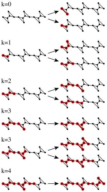
Figure 6: [color online] An example of the dimer assignment procedure for a separator $\Delta$ that is three cities wide. Initially, no edges are matched (left part of $k=0$). The first choice, $k=0$, is between the two edges inside $\Delta$ that are incident upon the far left node. In the example shown, the lower bond (connecting node 0 to node 2; see Fig. 3) is chosen, as shown on the left of the $k=1$ section of the figure. At this stage, one has computed matrices $A_{1}$, $M_{1}$, and $V_{1}$. The comparison of the next two possible matchings, shown on the right part of the $k=1$ subfigure, compares the inclusion of the $(q,r)=(3,5)$ and $(3,4)$ edges. In some cases, as in the first $k=3$ panel, a choice is forced and $A_{k}$, $M_{k}$, and $V_{k}$ need not be updated. The $k=4$ choices are forced, as an even number of domain walls must cross the separator, so that an even number of the top nodes and an even number of the bottom nodes are unmatched.

As $\operatorname{Pf}(A_{k})=\prod_{i=1,..,k}z_{i}$, the factor $z_{k+1}$ is the ratio $\operatorname{Pf}(A_{k+1})/\operatorname{Pf}(A_{k})$ of the Pfaffians that is needed to apply Eq. (17). Hence, this update in the factorization allows us to find the probability $x_{q_{k+1},r_{k+1}}z_{k+1}(q_{k+1},r_{k+1})$ of selecting the specific edge $(q_{k+1},r_{k+1})$ to augment the matching. Once we have chosen a match for $q_{k+1}$, we then update $A_{k}$ to $A_{k+1}$ from $K^{-1}$, $V_{k}$ using $z_{k+1}$, and $M_{k}$ using Eq. (25). This process is repeated until a maximal (though usually not complete) matching within $\Delta$ is obtained. With our choice of Fisher cities, there are only two candidates $r_{k+1}$ for each $q_{k+1}$ when using fixed boundary conditions; for periodic boundary conditions (Sec. IV), matching the initial node $q_{1}=0$ requires the comparison of three choices. Note that not all the $z$ need be computed as the total probability sums to unity; when considering two choices, considerable time is saved by computing the probability of only one of the choices. An example of dimer assignment is depicted in Fig. 6.

The results derived by Wilson for the bounds on the number of steps using Gaussian elimination carry over directly to the approach using Pfaffian elimination. The maximal size of the separator is of order $O(L)=O(n^{1/2})$. There are $O(n^{3/2})$ operations in the dimer assignment for the largest separator: matching a single dimer requires at most $O(n)$ steps, due to the multiplication of matrices of size $2\times O(n^{1/2})$ by matrices of size $O(n^{1/2})\times O(n^{1/2})$, and there are $O(n^{1/2})$ matchings in each separator. Calculating $K^{-1}$ also requires $O(n^{3/2})$ steps. As the smaller separators decrease in size geometrically, as the sample is subdivided, the number of operations for each of the smaller separators decreases geometrically, and the sum of steps over all levels of the nested dissection gives a total of $O(n^{3/2})$ arithmetic steps to generate a random assignment. The running time then is a product of the time per operation, which depends on the needed precision, and this number of steps. As discussed in more detail in Sec. III.5, the running time grows roughly linearly with the precision: the necessary precision grows only slowly with $n$, but proportionally to $\beta$.

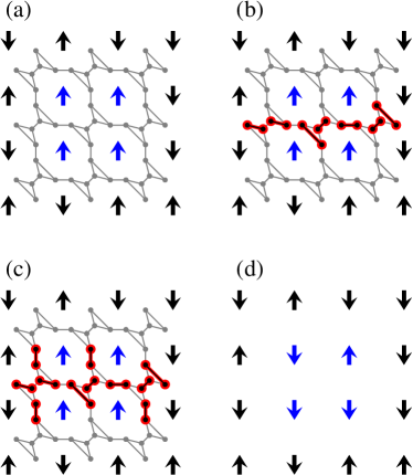
Figure 7: [color online] Application of the result of the example dimer assignment from Fig. 6 to the spin assignment. (a) The initial spin configuration, with fixed spins on the boundary. The portion of $G$ used to compute $K$, $[K^{-1}]_{\Delta}$ and the dimer assignment is indicated in gray. The middle row of Fisher cities composes $\Delta$, the dimer separator. (b) The sample dimer assignment (partial matching) for $\Delta$ from Fig. 6 superimposed on $G$. (c) Extra choices in the matching are forced by the matching internal to $\Delta$. These additional dimers cut across the bonds separating spins in $D$, the two spin rows parallel to $\Delta$. (d) In the last step, the modifiable spins are updated. The update is based upon the portion of domain walls forced by the partial matching in (c). Moving from left to right, for example, from the two fixed spins on the middle of the left side, a spin is reversed if an odd number of dimers extending from $\Delta$ are crossed.

Once all nodes in the separator $\Delta$ have dimers associated with them, the broken bonds along the strip $D$ of the Ising system are found from the locations of the dimers between these cities and the neighboring ones. We can then directly assign the spins along the strip. An example of such a spin assignment is displayed in Fig. 7.

III.4 Verification

The structure of the calculation is rather complex, so we verified our implementation of the algorithm in several ways. We checked exact partition function calculations for pure systems against the results of our computation. Exact enumeration for pure and disordered samples in systems up to $n=5^{2}$ was used to predict sampling probabilities: we then used our code to generate over $10^{5}$ samples and compared the sampled probability distribution with the exact calculations. These were in statistical agreement. Each author of this paper developed a code independently: these were compared on the same Gaussian spin glass samples of size $33^{2}$ and found to generate the same distribution for configurations, at low temperatures, also consistent with the Boltzmann distribution for total energy. At low temperatures, the sampled configurations approached those of the ground state configurations (which were predicted using an independent ground state code based on combinatorial optimization methods Barahona ; GSKastCities ).

III.5 Data types and timing

Our code is constructed so that the data type of matrix elements can be any field (double precision numbers, multiple-precision numbers, or exact rationals, for example). This allows us to check the effects of the choice of numerical type on the accuracy, stability, and running time of the sampling algorithm. For higher precision variables, we use the GMP library GMP for exact rational arithmetic and either the MPFR MPFR extension to GMP or the GMP library itself for multiple-precision floating point arithmetic. We find that the latter two floating point types give comparable performance and accuracy. Using exact rationals allows for mathematically exact sampling, but results in a temperature-dependent slowdown by a factor of $10$ or $100$ over the range of temperatures, $T=0.1$ to $T=1$, we used while comparing rationals with floating point calculations.

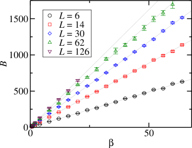
Figure 8: [color online] The plot shows the sample averages of the number of bits of precision $B_{\mathrm{a}vg}$ required to obtain the correct sampling, for system sizes $n=L^{2}=6^{2}$ through $126^{2}$ with fixed boundaries, as a function of inverse temperature $\beta$, for Gaussian disorder. The lines indicate linear fits of the form $B_{\mathrm{a}vg}=c\beta$. The number of bits needed for periodic boundary conditions (not shown) are very close to these same lines, at each system size. To find an accurate result with high confidence, one can use twice the average needed value: this was sufficient for all samples ($>10^{4}$) that we examined.

The edges $u$ are chosen by comparing the probability $P(p,u\,|\,p)$ with a random number chosen in the interval $\left[0,1\right)$. The sequence of random numbers and computed probabilities determines the spin configuration selected. We determine the needed precision for a given sample and temperature by demanding that the result of a specific assignment be independent of the precision, for a given sequence of random numbers. Note that using this precision does not give the exact values of the probabilities at each stage of the computation, but the sampling does not change at increased precision. If a number in the sequence happens to be extremely close to the computed probability, higher precision arithmetic could be required.

Results of our tests for needed precisions are summarized in Fig. 8, where we plot the number of bits needed, determined by bisection in the number of bits, averaged over random number sequences and disorder. We find that the distribution of the required number of bits is not very broad, regardless of temperature and disorder realization $\mathcal{J}$. Less than $10^{-4}$ of the attempts require more than double the average precision to find the correct sampling. Hence fixing the precision at two to three times the average value will almost guarantee an exact sampling.

For high temperatures (of order $T=1$), low precisions (i.e. fixed double precision variables) are sufficient for the system sizes we study (see Fig. 9). For lower temperatures, higher precisions are needed. The needed precision is well fit by a linear growth in $\beta$, for $\beta>0.5$. This is consistent with the expectation that, as the weights vary as $\exp(-\beta J)$, the number of bits needed to describe the weights grows linearly with $\beta$, for fixed typical values of $J$. The number of needed bits grows only slowly with $L$. This is consistent with the structure of the sampling and Pfaffian computation, which are hierarchical in structure, so that the accumulated error grows only slowly with $L$.

For systems up to size $64^{2}$, $600$ bits of precision are sufficient for temperatures $T>0.1$. For larger systems and lower temperatures, more bits are needed. For example, we use 2048 bits to reliably sample configurations at $\beta=25$ and $L=128$.

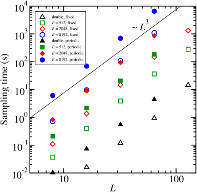
Figure 9: [color online] Run time, measured in seconds, to generate a single configuration, as a function of system size $L$, using a 2.4 GHz Intel Core 2 Duo processor (MacBook Pro). Double precision (64 bit floating point) data is indicated with triangles, while multi-precision results for $B=512$, 2048, and 8192 bits are indicated by squares, diamonds, and circles, respectively. Samples are generated for $L\leq 128$ with fixed boundaries (closed symbols) and for $L\leq 64$ with periodic boundaries (filled symbols). The sample-to-sample fluctuation of disorder realization is less than 0.1% of the run time, so error bars are not shown. The solid line indicates the form of the expected dependence of run time on system size for a given fixed precision, that is, $\sim L^{3}$.

We collected timing data for the performance of our algorithm as a function of system size and temperature. These data are summarized in Fig. 9. We find that sampling with periodic boundary conditions (Sec. IV) takes approximately 5.5-6.5 times longer than sampling with fixed boundary conditions. The needed precision and running times for $\pm J$ disorder are very close to those shown in Figs. 9 and 8. For $64<B<512$, the run time to sample a configuration varies only slowly with $B$, approximately by a factor of $1.5$ over this range. For higher precision, the running time grows somewhat faster than linearly with $B$, and hence somewhat faster than linearly with $\beta$.

IV Periodic Boundary Conditions

Fixed boundary conditions are appropriate for patchwork dynamics, but, for other simulations, other boundary conditions, may be useful. One simple way to implement open boundary conditions is to set to zero all the $J_{ij}$ connecting interior to boundary spins. For cylindrical samples with open boundaries, we use a “separator” which does not actually separate the graph, but one that slices the sample perpendicular to the circumference of the cylinder, resulting in a simple planar graph with fixed boundaries. Toroidal graphs require a more complicated sampling scheme, as they are not planar. In general, for a graph of genus $g$, the partition function of the dimer problem may be calculated exactly by summing $4^{g}$ Pfaffians KastTorus . The reasoning behind this summation can be adapted to sampling for periodic spin lattices.

IV.1 Partition function on the periodic lattice

The Kasteleyn matrix approach for computing $Z$ can be extended to handle the periodic case, by adding connections between cities that complete the periodic boundaries, converting the planar square sample to a toroidal one, but the direct correspondence between dimer configurations and spin configurations is affected. On the torus, topologically non-trivial domain walls must always come in pairs, or the spin configuration can not be consistently defined. But the matching problem allows for odd numbers of loops to wrap around the torus on either axis. For $T=0$ ground states, one can decide to ignore this fact and allow variable boundary conditions, which allow for an odd number of domain walls relative to other boundary conditions. Choosing the boundary condition and spin configuration that jointly minimize $\mathcal{H}$ gives the extended ground state construction KastCities . At finite temperature with fixed boundary conditions, however, we need to arrange for the cancellation of dimer configurations which would imply an odd number of domain walls that wrap around either axis.

	$\operatorname{Pf}(K^{++})$	$\operatorname{Pf}(K^{+-})$	$\operatorname{Pf}(K^{-+})$	$\operatorname{Pf}(K^{--})$
(e,e)	+	+	+	+
(o,e)	-	-	+	+
(e,o)	-	+	-	+
(o,o)	-	+	+	-

Table 1: A table of the signs for different combinations of spanning loop parities in the dimer model for each of the four Pfaffians $K^{\pm\pm}$ for the torus. The set of loops found from a dimer configuration can have a total wrapping number that is odd (o) or even (e) number along either the horizontal or vertical directions. This gives four possible classes of dimer configurations (e,e), (e,o), (o,e) and (o,o). For the dual mapping used here, the physical spin configurations for the Ising model are restricted to those with an even number of domain walls wrapping in both directions, i.e., the (e,e) class. The four classes of dimer configurations are summed in each Pfaffian of the four Kasteleyn matrices, $K^{\pm\pm}$, with a sign that depends on the class and the matrix. These four matrices assign different signs to the weights of the dual edges that connect the boundaries together, with a $+$ or $-$ sign for each of the two types of boundary connections, i.e., horizontal or vertical. Applying this table, we get the partition function for the valid dimer configurations by the sum $Z=[\operatorname{Pf}(K^{++})+\operatorname{Pf}(K^{+-})+\operatorname{Pf}(K^{-+})+\operatorname{Pf}(K^{--})]/2$, which counts only the (e,e) class of dimer configurations. This sum differs from the more commonly studied case, the dimer model using cities on the primal lattice, where all classes of matchings are valid configurations and $Z=[-\operatorname{Pf}(K^{++})+\operatorname{Pf}(K^{+-})+\operatorname{Pf}(K^{-+})+\operatorname{Pf}(K^{--})]/2$ gives the sum over (e,e), (o,e), (e,o), and (e,e).

This cancellation is achieved by summing over four Pfaffians, in a fashion similar to that developed for the primal lattice KastCities , though the details differ for the dual lattice. The four Pfaffians correspond to four possible choices of sign for the elements of $K(q,r)$ that complete the periodic connections. That is, the values of $K(q,r)$ for edges that connect the last column to the first column (that wrap around in the $x$ direction) are uniformly set to one of two choices, $\pm\exp[-\beta w(q,r)]$, and the values for the edges that connect the last row to the first row (that wrap around in the $y$ direction) are also uniformly set, independent of the choice for the $x$-wrapping bonds, again to $\pm\exp[-\beta w(q,r)]$. This gives four matrices, $K^{++}$, $K^{-+}$, $K^{+-}$, and $K^{--}$. The dimer configurations that are summed up in the Pfaffians enter with different relative signs, depending on how many times the matchings wrap around each axis, as the parity of the windings affects the sign of the dimer configurations when the negative sign is chosen for the periodically-connecting edges. The effects of these signs are tabulated and explained in Table 1. The sum of the Pfaffian of these four matrices then gives twice the partition function, as those dimer configurations with an even number of wrapping loops enter four times and those with an odd number, in either direction, are cancelled out, and there is a two-to-one mapping of spin configurations to domain walls in the periodic case (due to global spin flip symmetry).

IV.2 Matching probabilities for the torus

There are several simple possible choices for a nested dissection for toroidal samples of dimension $L\times L$. The number of cities is the same as the number of variable spins, i.e., $L^{2}$. We chose to use a horizontal strip of length $L$ in the first row of cities, which fixes the spins in the first two rows, followed by a vertical strip in of length $L-1$ in the first column, which fixes the first two columns of spins, followed by a sampling the remaining $(L-1)\times(L-1)$ cities, i.e., a sampling of the remaining $(L-2)\times(L-2)$ spins using the already determined spins in the first two columns and rows as fixed spin boundary conditions. The first two “separators” don’t divide the sample into separate pieces, but instead provide for the cutting of loops that wind around the torus, in two stages.

For the first sampling, the periodic horizontal row, one has to sample using four Kasteleyn matrices in parallel. For the second sampling, on a cylindrical geometry, one needs to find probabilities by summing over two Kasteleyn matrices $K^{+}$ and $K^{-}$, in order to eliminate domain walls that wrap around the cylinder an odd number of times. We can consider both cases as specific examples of a general problem: sampling using multiple Kasteleyn matrices simultaneously.

For this general case, consider a partition function $Z$ that is found by summing the Pfaffian over matrices $K^{\alpha}$, with weights $q_{\alpha}$ (e.g., $\alpha={\pm\pm}$ and $q_{\alpha}=\frac{1}{2}$ for toroidal boundary conditions). The partition function is then

$$Z=\sum_{\alpha}q_{\alpha}K^{\alpha}\ .$$ (27)

The computation of probability of selection is more complicated than for the case of a single $K$. For each $K^{\alpha}$, we consider the inverse indexed by elements of the separator $\Delta$, $[(K^{\alpha})^{-1}]_{\Delta}$, and inductively factorize $[(K^{\alpha})^{-1}]_{p}$ for our current choice of sampled edges $p=\{e_{1},\ldots,e_{k}\}$. The conditional probability of choosing edge $e_{k+1}$, simplifying the notation by writing $u$ for $e_{k+1}$ and using $z^{\alpha}(e)$ to denote $z^{\alpha}_{k}$ for edge $e=(q_{k},r_{k})$, is then given by

$$P(p,u\,|\,p) = \frac{Z_{p,u}}{Z_{p}}$$

$$= \frac{\sum_{\alpha}q_{\alpha}\operatorname{Pf}(K_{p,u}^{\alpha})\prod_{e\in p,u}x^{\alpha}(e)}{\sum_{\alpha}q_{\alpha}\operatorname{Pf}(K_{p}^{\alpha})\prod_{e\in p}x^{\alpha}(e)}$$

$$= \frac{\sum_{\alpha}q_{\alpha}\operatorname{Pf}([(K^{\alpha})^{-1}]_{p,u})\operatorname{Pf}(K^{\alpha})\prod_{e\in p,u}x^{\alpha}(e)}{\sum_{\alpha}q_{\alpha}\ Pf([(K^{\alpha})^{-1}]_{p})\operatorname{Pf}(K^{\alpha})\prod_{e\in p}x^{\alpha}(e)}$$

$$= \frac{\sum_{\alpha}q_{\alpha}\operatorname{Pf}(K^{\alpha})\prod_{e\in p,u}z^{\alpha}(e)x^{\alpha}(e)}{\sum_{\alpha}q_{\alpha}\operatorname{Pf}(K^{\alpha})\prod_{e\in p}z^{\alpha}(e)x^{\alpha}(e)}\$$

$$= \frac{\sum_{\alpha}\zeta_{\alpha}(p)z^{\alpha}(u)x^{\alpha}(u)}{\sum_{\alpha}\zeta_{\alpha}(p)}\,,$$

where

$$\zeta_{\alpha}(p)=\operatorname{Pf}(K^{\alpha})\prod_{e\in p}\frac{x^{\alpha}(e)z^{\alpha}(e)}{|x^{\alpha}(e)|}\ .$$ (29)

This extra weighting quantity, $\zeta_{\alpha}(p)$, is not needed for planar samples, due to cancellations, but is required here to allow for the different $p$-dependent weightings resulting from the distinct boundary conditions. It incorporates the weight of the whole $K^{\alpha}$ matrix, the modification of those weights by the factors of $z^{\alpha}(e)$ resulting from the choice of edges in $p$, and the sign of the weights (the magnitudes are identical in each $\alpha$ for a given choice of $p$ and hence cancel out). This weighting factor can be updated at each stage $k$ along with the set of $V^{\alpha}_{k}$, $M^{\alpha}_{k}$, and $A^{\alpha}_{k}$ for each $\alpha$. In the case of the periodic lattice, these four sets of matrices are updated and used to compute the values of $z^{\alpha}(e)$ to find the conditional probabilities.

IV.3 Sampling spins

The dimer assignments are carried out on $G$ for the periodic case using Eq. (IV.2). To finally carry out the sampling on the torus, one first arbitrarily sets the value of an initial spin, the spin at the upper left corner, i.e., at location $(0,0)$. The spin at the left side of the second row, at location $(1,0)$, is fixed by the first element of the matching for the first separator. This is the exceptional case for this lattice where one has three choices for the matching edge on $G$ ($(0,1)$, $(0,2)$, and $(0,6L-2)$). After this choice has been made, the rest of the spins in the first two rows are then assigned as in the fixed boundary case. An example of the relative domain wall density for a $64^{2}$ periodic sample is displayed in Fig. 10. This plot shows the variance $\mu_{ij}(1-\mu_{ij})$ in the bond satisfaction, where $\mu_{ij}$ is the probability of a given bond being satisfied, i.e., $s_{i}s_{j}J_{ij}>0$.

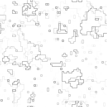
Figure 10: Relative domain walls found in an individual 2D Ising spin glass sample with $64^{2}$ spins, periodic boundary conditions, and unit variance Gaussian disorder, for temperature $T=0.16$. The bond satisfaction probabilities were estimated by averaging over 660 samples. As in Fig. 1, the lines indicate the probability of relative domain walls between two configurations: the darkest lines indicate where the bond dual to that domain wall has a nearly 50% chance of opposite or equal relative orientations; where there is no line or a light line separating two spins, the two spins have a very high probability of a single relative orientation, either aligned or opposite.

IV.4 Running time

We find that the number of bits required for the periodic case increases only by a small amount, about 1%, over the planar case for samples of the same size. Carrying out the initial Pfaffian elimination for single $\alpha$ for the entire sample is slower than for the planar case, as there are about four times as many operations, but this computation requires only a small fraction of the time in any case. However, as the periodic case requires the maintenance of four $V_{k}$, $A_{k}$, and $M_{k}$ matrices, sampling in the periodic case is slower than for the fixed boundary case. We find that sample generation is about $5.5$ times slower for periodic samples, compared with planar samples, for $L=16$ through $L=64$.

V Concluding comments

In this paper, we have described an algorithm that generates spin configurations for the 2D Ising spin glass, where the samples generated are directly selected according to the equilibrium probability distribution. This method follows from Wilson’s dimer sampling algorithm, though we have modified the matrix algebra for speed and simplicity, and have adopted the dimer matching to the study of the Ising spin glass. We have also generalized the method to periodic samples.

We note that as the inverse Kasteleyn matrix contains the dimer-dimer correlation functions along the separator, one need not carry out all of the sampling steps to compute domain wall densities. One can directly examine the inverse on the separator to find the domain wall densities on a single separator, by stopping at step 4 of the outline in Sec. III. The separator can then be changed to compute the bond satisfaction probabilities in each row of the sample. Sampling configurations provides more information, but if the bond satisfaction variance is all that is needed, this approach is more precise and is not unreasonably slow.

This algorithm can also be used to directly and uniformly sample ground states in the 2D $\pm J$ spin glass model. At low enough temperatures (on the order of $T\approx 0.1$), the ground states occur frequently, as can be confirmed by their energies being lowest or by comparison with a ground state energy found by combinatorial optimization. The statistics of the ground state configurations can therefore be directly sampled (by rejecting other states when they occur), exactly, using this algorithm.

Our implementation of the sampling algorithm is efficient enough to allow for rapid enough sampling to study finite temperature patchwork dynamics out to patch sizes $\ell$ of at least $\ell=32$. Large numbers of samples can be comfortably generated for $L=64$ and $T<0.01$ or for $L=128$ and $T=0.04$. This should allow for more conclusive studies on the Gaussian and $\pm J$ spin glass problems in two dimensions.

We thank Jan Vondrak for sharing his code for computing the partition function of the $\pm J$ spin glass model and Simon Catterall for sharing his code for computing Pfaffians. This work was supported in part by the NSF under grant No. 0606424.

References

- (1) K. Binder and A. P. Young, Rev. Mod. Phys. 38, 801 (1986).
- (2) “Spin Glasses and Random Fields”, A. P. Young, ed. (World Scientific, Singapore, 1998).
- (3) V. Dupuis, F. Bert, J.-P. Bouchaud, J. Hammann, F. Ladieu, D. Parker and E. Vincent, Pramana J. Phys. 64, 1109 (2005)
- (4) D. S. Fisher and D. A. Huse, Phys. Rev. Lett. 56, 1601 (1986); D. S. Fisher and D. A. Huse, Phys. Rev. B 38, 373 (1988).
- (5) G. Parisi, Phys. Rev. Lett. 43, 1754 (1979).
- (6) A. P. Young and H. G. Katzgraber, Phys. Rev. Lett. 93, 207203 (2004); H. G. Katzgraber, M. Körner and A. P. Young, Phys. Rev. B, 73, 224432 (2006).
- (7) H. Rieger, G. Schehr and R. Paul, Prog. Theor. Phys. Suppl. 157, 111 (2005).
- (8) A. Sicilia, J. J. Arenzon, A. J. Bray and L. F. Cugliandolo, Phys. Rev. E 76, 061116 (2007).
- (9) F. Belletti, M. Cotallo, A. Cruz, L. A. Fernandez, A. Gordillo-Guerrero, M. Guidetti, A. Maiorano, F. Mantovani, E. Marinari, V. Martin-Mayor, A. Munoz Sudupe, D. Navarro, G. Parisi, S. Perez-Gaviro, J. J. Ruiz-Lorenzo, S. F. Schifano, D. Sciretti, A. Tarancon, R. Tripiccione, J. L. Velasco and D. Yllanes, Phys. Rev. Lett. 101 157201 (2008).
- (10) F. Edwards and P. W. Anderson, J. Phys. F 5, 965 (1975).
- (11) J. Houdayer and O. C. Martin, Phys. Rev. Lett. 83, 1030 (1999).
- (12) A. K. Hartmann and A. P. Young, Phys. Rev. B 66, 094419 (2002); C. Amoruso and A. K. Hartmann, Phys. Rev. B 70, 134425 (2004); O. Melchert and A. K. Hartmann, Phys. Rev. B 76 174411 (2007).
- (13) F. Liers, M. Jünger, G. Reinelt and G. Rinaldi, in “New Optimization Algorithms in Physics”, A. K. Hartmann and H. Rieger, eds. (Wiley-VCH, Weinheim, 2004).
- (14) M. Palassini and A. P. Young, Phys. Rev. Lett. 85, 3017 (2000).
- (15) S. Boettcher and A. G. Percus, Phys. Rev. Lett. 86, 5211 (2001).
- (16) C. K. Thomas, O. L. White and A. A. Middleton, Phys. Rev. B 77 092415 (2008).
- (17) D. B. Wilson, Proc. 8th Symp. Discrete Algorithms 258, (1997).
- (18) F. Barahona, J. Phys. A 15 3241 (1982).
- (19) P. W. Kasteleyn, J. Math. Phys. 4, 287 (1963).
- (20) H. G. Katzgraber and L. W. Lee, Phys. Rev. B 71 134404 (2005); T. Jörg, J. Lukic, E. Marinari and O. C. Martin, Phys. Rev. Lett. 96 237205 (2006); H. G. Katzgraber, L. W. Lee and I. A. Campbell, Phys. Rev. B 75 014412 (2007); A. K. Hartmann, Phys. Rev. B 77 144418 (2008).
- (21) M. Kac and J. C. Ward, Phys. Rev. 88, 1332 (1952).
- (22) M. E. Fisher, J. Math. Phys. 7, 1776 (1966).
- (23) P. D. Beale, Phys. Rev. Lett. 76, 78 (1996).
- (24) L. Saul and M. Kardar, Phys. Rev. E 48 R3221 (1993).
- (25) A. Galluccio, M. Loebl and J. Vondrak, Phys. Rev. Lett. 84, 5924 2000.
- (26) J. A. Blackman and J. Poulter, Phys. Rev. B 44, 4374 (1991).
- (27) J. Lukic, A. Galluccio, E. Marinari, O. C. Martin, G. Rinaldi, Phys. Rev. Lett. 92, 117202 (2004).
- (28) W. Janke, Math. Comput. Simulat. 47 329 (1998).
- (29) H. Rieger, L. Santen, U. Blasum, M. Diehl, M. Jünger, G. Rinaldi, J. Phys. A 29, 3939 (1996).
- (30) R. H. Swendsen and J.-S. Wang, Phys. Rev. Lett. 57, 2607 (1986); J. Houdayer, Eur. Phys. J. B 22, 479 (2001); J.-S. Wang, Phys. Rev. E 72, 036706 (2005).
- (31) J. G. Propp and D. B. Wilson, Random Struct. Algorithms 9, 223 (1996).
- (32) C. Chanal and W. Krauth, Phys. Rev. Lett. 100 060601 (2008).
- (33) M. Sasaki and O. C. Martin, Phys. Rev. Lett. 91 097201 (2003).
- (34) T. Jörg and H. G. Katzgraber, Phys. Rev. Lett. 101 197205 (2008).
- (35) W. Krauth, “Statistical Mechanics: Algorithms and Computations” (Oxford University Press, 2006).
- (36) D. Randall and D. Wilson, Proc. 10th Symp. Discrete Algorithms 959, (1999).
- (37) J. Propp, Theoretical Computer Science 303, 267 (2003).
- (38) C. Zeng, P. L. Leath and T. Hwa, Phys. Rev. Lett. 83 4860 (1999).
- (39) Y. L. Loh and E. W. Carlson, Phys. Rev. Lett. 97 227205 (2006).
- (40) C. K. Thomas and A. A. Middleton, Phys. Rev. B 76 220406(R) (2007).
- (41) H. S. Robertson, “Statistical Thermophysics” (Prentice Hall, 1993).
- (42) R. J. Lipton, D. J. Rose and R. E. Tarjan, SIAM J. Numer. Analysis 16 316 (1979).
- (43) M. Bajdich, L Mitas, L. K. Wagner, K. E. Schmidt, Phys. Rev. B 77, 115112 (2008).
- (44) M. Ishikawa, M. Wakayama, J. Comb. Th. (113), 113 (2006).
- (45) I. S. Duff, Proc. IEEE 65 500 (1977).
- (46) See the manual by T. Granlund at http://gmplib.org.
- (47) L. Fousse, G. Hanrot, V. Lefèvre, P. Pélissier, P. Zimmerman, ACM Trans. Math. Software 33, 13 (2007).
- (48) P. W. Kasteleyn, Physica 27 1209 (1961).