Simulation of a particle-laden turbulent channel flow using an improved stochastic Lagrangian model

Abstract

The purpose of this paper is to examine the Lagrangian stochastic modeling of the fluid velocity seen by inertial particles in a non-homogeneous turbulent flow. A new Langevin-type model, compatible with the transport equation of the drift velocity in the limits of low and high particle inertia, is derived. It is also shown that some previously proposed stochastic models are not compatible with this transport equation in the limit of high particle inertia. The drift and diffusion parameters of these stochastic differential equations are then estimated using DNS data. It is observed that, contrary to the conventional modeling, they are highly space-dependent and anisotropic. To investigate the performance of the present stochastic model, a comparison is made with DNS data as well as with two different stochastic models. A good prediction of the first and second order statistical moments of the particle and fluid seen velocities is obtained with the three models considered. Even for some components of the triple particle velocity correlations, an acceptable accordance is noticed. The performance of the three different models mainly diverges for the particle concentration and the drift velocity. The proposed model is seen to be the only one which succeeds in predicting the good evolution of these latter statistical quantities for the range of particle inertia studied.

I Introduction

In the past years, several numerical methods have been employed to study the dispersion of solid particles in turbulent flows. Generally, small enough particles are considered in order to treat them as point-particles.Maxey and Riley (1983); Reeks (1977); McLaughlin (1989); Rouson and Eaton (2001) Assuming that the drag force is only of importance, the link between the motion of an inertial particle and the carrier fluid is given by the following system of equations :

$$\frac{dx_{p,i}}{dt}=v_{p,i},$$ (1)

$$\frac{dv_{p,i}}{dt}=\frac{\tilde{u}_{i}-v_{p,i}}{\tau_{p}}\,,$$ (2)

where $x_{p,i}$ and $v_{p,i}$ are the particle position and velocity, $\tau_{p}$ is the particle relaxation time which is expressed in terms of the drag coefficient and of the magnitude of the relative velocity, and $\tilde{u}_{i}=u_{i}(\mathbf{x}_{p},t)$ is the fluid velocity at the particle location. Under these considerations, the main difficulty then lies in the proper computation of the fluid velocity at each particle location. The first possibility is to use Direct Numerical Simulation (DNS).McLaughlin (1989); Ferrante and Elghobashi (2003) This technique gives the best estimation of the fluid velocity seen by particles. Nevertheless, it necessitates very high computational ressources. A more affordable numerical way is provided by Large Eddy Simulation (LES).Marchioli et al. (2008a) Contrary to DNS, a model which takes the residual fluid dynamic (i.e. at the sub-grid scale) into account should be used to predict the instantaneous fluid velocity seen by particles. Finally, when the computational cost of this latter technique is still too high, it is then possible to make use of macroscopic numerical simulation such as Reynolds-Averaged Navier-Stokes (RANS). The use of a RANS-Lagrangian method to describe the motion of solid particles in a turbulent two-phase flow necessitates to generate the fluctuating velocity of the carrier phase at particle location.Mashayek and Pandya (2003) In this framework, averaged quantities such as the mean velocity and some of the mean turbulent characteristics of the carrier phase are determined by solving the Reynolds-Averaged Navier-Stokes equations. The time integration of the equations governing the motion of inertial particles [Eqs. (1) and (2)] requires the knowledge of the instantaneous velocity of the fluid at the particle location. The reconstruction of the random nature of the fluctuations along inertial particle trajectories can be achieved, for instance, using a stochastic Lagrangian models.Simonin et al. (1993); Oesterlé and Zaichik (2004); Iliopoulos and Hanratty (2004); Reeks (2005); Pialat et al. (2007); Dehbi (2008) Most of these models for the simulation of turbulent two-phase flows involves specific formulations based on the Langevin model which can be written in a general form as :

$$d\tilde{u}_{i}=A_{i}dt+B_{ij}dW_{j}\,,$$ (3)

for the instantaneous fluid velocity at particle location. In this latter stochastic differential equation (SDE), $A_{i}$ is the drift vector, $B_{ij}$ is the diffusion matrix, and $dW_{j}$ are the increments of a vector-valued Wiener process with independent components. Some important properties of these increments are that they are non-differentiable and normally distributed with mean $\left\langle W_{i}(t+dt)-W_{j}(t)\right\rangle=0$ and variance $\left\langle\left[W_{i}(t+dt)-W_{j}(t)\right]^{2}\right\rangle=dt\,\delta_{ij}$.Gardiner (1997) In order to predict the fluid velocity seen by inertial particles, one has to model the drift vector and the diffusion matrix. In the present study, we focus on the models for the drift vector proposed by Simonin et al. (1993)

$$A_{i}=-\frac{1}{\rho_{f}}\frac{\partial\left\langle p\right\rangle}{\partial x_{i}}+\nu\frac{\partial^{2}\left\langle u_{i}\right\rangle}{\partial x_{j}\partial x_{j}}+\left(v_{p,j}-\tilde{u}_{j}\right)\frac{\partial\left\langle u_{i}\right\rangle}{\partial x_{j}}+G_{ij}\left(\tilde{u}_{j}-\left\langle u_{j}\right\rangle\right)\,,$$ (4)

and by Minier and Peirano (2001)

$$A_{i}=-\frac{1}{\rho_{f}}\frac{\partial\left\langle p\right\rangle}{\partial x_{i}}+\nu\frac{\partial^{2}\left\langle u_{i}\right\rangle}{\partial x_{j}\partial x_{j}}+\left(\left\langle v_{p,j}\right\rangle-\left\langle\tilde{u}_{j}\right\rangle\right)\frac{\partial\left\langle u_{i}\right\rangle}{\partial x_{j}}+G_{ij}\left(\tilde{u}_{j}-\left\langle u_{j}\right\rangle\right)\,.$$ (5)

In these expressions, $\nu$ is the kinematic viscosity, $\rho_{f}$ is the fluid density, $p$ stands for the pressure, $u_{i}$ is the fluid velocity, $v_{p,i}$ is the solid particle velocity and $G_{ij}$ is the drift matrix. The difference between both models lies in the form of the third term which describes the crossing-trajectory effect.Csanady (1963) In the model proposed by Simonin et al. (1993), this term is written as a function of the instantaneous relative velocity between the particle and the fluid while Minier and Peirano (2001) suggested to express it as a function of the mean relative velocity.
It has to be noted that in the limit of low particle inertia ($\tau_{p}\ll 1$), both models give the well-known Generalized Langevin Model (GLM) derived by Pope (1983) to predict the motion of fluid particle in a turbulent flow. Nevertheless, as it will be shown in Sec. II, these two previous stochastic models are not compatible with the transport equation of the drift velocity (mean fluctuating fluid velocity at particle location) for large particle inertia. In order to correct this discrepancy, a new form of the drift vector is proposed. In Sec. III, the method used to derive the drift and diffusion parameters of these stochastic models is described, and the estimated values obtained using DNS data are presented. The performance of the proposed functional form of the drift vector is then assessed by comparison with DNS data in Sec. IV. Finally, concluding remarks are given in the last section.

II Exact and modeled transport equations of the drift velocity

In this section, we study the Langevin models proposed by Simonin et al. (1993) and Minier and Peirano (2001) through the transport equation of the drift velocity in the limit of low and high particle inertia. Based on this study, a new model for the drift vector $A_{i}$ is proposed.

II.1 Degenerate equations for low and high particle inertia

Let us consider the gas-solid flow from an Eulerian (macroscopic) point of view. The exact transport equation for the statistical moments of the particle and fluid seen velocities, as well as for the fluid seen-particle velocity correlations, can be derived, for example, from the transport equation of a joint probability density function for the particle and fluid seen velocities.Simonin (2000); Minier and Peirano (2001); Pandya and Mashayek (2003); Reeks (2005) The exact transport equation of the drift velocity, $\left\langle\tilde{u}^{\prime}_{i}\right\rangle=\left\langle\tilde{u}_{i}-\left\langle u_{i}\right\rangle\right\rangle$, can be written as Minier and Peirano (2001)

$$\alpha_{p}\rho_{p}\frac{\overline{D}_{p}}{Dt}\left\langle\tilde{u}^{\prime}_{i}\right\rangle= \alpha_{p}\rho_{p}\left[\frac{\partial}{\partial x_{j}}\left(\left\langle u^{\prime}_{i}u^{\prime}_{j}\right\rangle-\left\langle\tilde{u}^{\prime}_{i}v^{\prime}_{p,j}\right\rangle\right)\right]-\left\langle\tilde{u}^{\prime}_{i}v^{\prime}_{p,j}\right\rangle\frac{\partial}{\partial x_{j}}\left(\alpha_{p}\rho_{p}\right)$$

$$-\alpha_{p}\rho_{p}\left(\left\langle v_{p,j}\right\rangle-\left\langle\tilde{u}_{j}\right\rangle\right)\frac{\partial\left\langle u_{i}\right\rangle}{\partial x_{j}}-\alpha_{p}\rho_{p}\left\langle\tilde{u}^{\prime}_{j}\right\rangle\frac{\partial\left\langle u_{i}\right\rangle}{\partial x_{j}}$$

$$-\alpha_{p}\rho_{p}\left(-\frac{1}{\rho_{f}}\frac{\partial\left\langle p\right\rangle}{\partial x_{i}}+\nu\frac{\partial^{2}\left\langle u_{i}\right\rangle}{\partial x_{j}\partial x_{j}}\right)+\alpha_{p}\rho_{p}\left\langle\frac{d\tilde{u}_{i}}{dt}\right\rangle\,,$$ (6)

where $\overline{D}_{p}(\cdot)/Dt=\partial(\cdot)/\partial t+\left\langle v_{p,j}\right\rangle\partial(\cdot)/\partial x_{j}$, and $\alpha_{p}$ is the particle volume fraction.
In the limit of vanishing particle inertia ($\tau_{p}\ll 1$), a solid particle behaves like a fluid particle tracer. Its velocity is equal to that of a fluid particle, the statistical moments of the fluid and particle velocities are thus identical. Moreover, the drift velocity is zero since this kind of particles samples homogeneously the turbulent flow field and the particle volume fraction is constant if the particles are uniformly distributed initially. As a consequence, it can be found, from equation (II.1), that the average of the time variation of the fluid velocity seen becomes equal to

$$\left\langle\frac{d\tilde{u}_{i}}{dt}\right\rangle=-\frac{1}{\rho_{f}}\frac{\partial\left\langle p\right\rangle}{\partial x_{i}}+\nu\frac{\partial^{2}\left\langle u_{i}\right\rangle}{\partial x_{j}\partial x_{j}}\,.$$ (7)

The averaged Navier-Stokes equations are thus recovered.
The opposite limit case, i.e. high particle inertia ($\tau_{p}\gg 1$), is also of great importance when studying gas-solid flows since the trajectories of such particles become completely independent of the fluid motion. In such a case, the particle velocity remains nearly identical to its initial value, the fluid seen-particle velocity correlations, the second and higher statistical moments of the particle velocity as well as the drift velocity tend to zero. Moreover, the particle volume fraction keeps a constant value across the fluid flow if particles are initially distributed uniformly. In the present study and without loss of generality, the velocity of these high inertia particles is considered identical to the mean fluid velocity. Under these considerations, it can be found from equation (II.1) that

$$\left\langle\frac{d\tilde{u}_{i}}{dt}\right\rangle=-\frac{1}{\rho_{f}}\frac{\partial\left\langle p\right\rangle}{\partial x_{i}}+\nu\frac{\partial^{2}\left\langle u_{i}\right\rangle}{\partial x_{j}\partial x_{j}}-\frac{\partial}{\partial x_{j}}\left\langle u^{\prime}_{i}u^{\prime}_{j}\right\rangle\,.$$ (8)

These two previous equations give the asymptotic limits of the average time derivative of the fluid velocity seen by particles. Besides, they can be used in order to verify that the Langevin models generally used to predict the evolution in time of this fluid velocity are correct in the limits of low and high particle inertia.
For example, let us consider first the model of the drift vector proposed by Simonin et al. (1993), i.e. equation (4). The average of equation (3) in the limit of low particle inertia yields

$$\left\langle\frac{d\tilde{u}_{i}}{dt}\right\rangle=-\frac{1}{\rho_{f}}\frac{\partial\left\langle p\right\rangle}{\partial x_{i}}+\nu\frac{\partial^{2}\left\langle u_{i}\right\rangle}{\partial x_{j}\partial x_{j}}\,,$$ (9)

since $\left\langle B_{ij}dW_{j}\right\rangle=0$. Thus, the model of the drift vector by Simonin et al. (1993) is able to produce the correct limit of the mean time increment of the fluid velocity seen in this particular case. When the particle inertia becomes high, the same expression is obtained from this model. In comparison with the exact one given by equation (8), it is noticed that the divergence of the Reynolds stress tensor is missing. Therefore, we can expect that some discrepancies could occur in the prediction of the momentum exchange between the dispersed and carrier phases for high particle inertia. Considering the model proposed by Minier and Peirano (2001), it can be seen that the expressions of the mean time increment of the fluid velocity seen in the limits of low and high particle inertia are identical to those obtained with the model of Simonin et al. (1993) This model is thus also not compatible with the transport equation of the drift velocity in the limit of high particle inertia. In the next section, a new model of the drift vector which makes possible the prediction of the theoretical limits given above is proposed.

II.2 Proposal of a new model

From the conclusions drawn in the previous section, we have designed a new model which gives the proper limits of the drift velocity transport equations in the cases of low and high particle inertia. This model for the drift vector $A_{i}$ is

$$A_{i}=-\frac{1}{\rho_{f}}\frac{\partial\left\langle p\right\rangle}{\partial x_{i}}+\nu\frac{\partial^{2}\left\langle u_{i}\right\rangle}{\partial x_{j}\partial x_{j}}+\left(v_{p,j}-\tilde{u}_{j}\right)\frac{\partial\left\langle u_{i}\right\rangle}{\partial x_{j}}+G_{ij}\left(\tilde{u}_{j}-\left\langle u_{j}\right\rangle\right)+\frac{\partial}{\partial x_{k}}\left(\left\langle\tilde{u}^{\prime}_{i}v^{\prime}_{p,k}\right\rangle-\left\langle u^{\prime}_{i}u^{\prime}_{k}\right\rangle\right)\,.$$ (10)

This drift vector is mainly different from those proposed by Simonin et al. (1993) and Minier and Peirano (2001) due to the presence of the term $\partial\left(\left\langle\tilde{u}^{\prime}_{i}v^{\prime}_{p,k}\right\rangle-\left\langle u^{\prime}_{i}u^{\prime}_{k}\right\rangle\right)/\partial x_{k}$ (i.e. the divergence of the difference between the fluid-particle covariances and the Reynolds stresses).

First, it has to be noted that in the limit of low particle inertia the model proposed is also identical to the GLM derived by Pope (1983) because $\left\langle\tilde{u}^{\prime}_{i}v^{\prime}_{p,k}\right\rangle\rightarrow\left\langle u^{\prime}_{i}u^{\prime}_{k}\vphantom{\tilde{u}^{\prime}_{i}v^{\prime}_{p,k}}\right\rangle$. In addition, the modeled averaged time increment of the fluid velocity seen using Eq. (10) has the proper limits since

$$\left\langle\frac{d\tilde{u}_{i}}{dt}\right\rangle=-\frac{1}{\rho_{f}}\frac{\partial\left\langle p\right\rangle}{\partial x_{i}}+\nu\frac{\partial^{2}\left\langle u_{i}\right\rangle}{\partial x_{j}\partial x_{j}}\,,$$ (11)

when $\tau_{p}\ll 1$, and

$$\left\langle\frac{d\tilde{u}_{i}}{dt}\right\rangle=-\frac{1}{\rho_{f}}\frac{\partial\left\langle p\right\rangle}{\partial x_{i}}+\nu\frac{\partial^{2}\left\langle u_{i}\right\rangle}{\partial x_{j}\partial x_{j}}-\frac{\partial}{\partial x_{j}}\left\langle u^{\prime}_{i}u^{\prime}_{j}\right\rangle\,,$$ (12)

for $\tau_{p}\gg 1$.
The introduction of a supplementary term, which is a function of the Reynolds stresses, in the drift vector has been motivated by the necessity for the stochastic model to be consistent with the transport equation of the drift velocity in the limit of high particle inertia. Nevertheless, this additional term had to vanish in limit of low particle inertia in order to keep the model similar to the GLM. This has naturally led us to add the fluid-particle covariance tensor which tends to the Reynolds stresses when $\tau_{p}\ll 1$ and to zero when $\tau_{p}\gg 1$. Moreover, incorporating the proposed model in the transport equation of the drift equation, it can be seen that this new term moment is physically consistent with the others.

At this point, we would like to emphasize the fact that the present model should be more suitable for predicting the fluid velocity seen by large solid particles than the models proposed by Simonin et al. (1993) and Minier and Peirano (2001), however, the presence of the fluid-particle covariances in the expression increases the degree of complexity of the stochastic model.

It is also worth mentioning that the SDE for the fluctuating fluid velocity seen derived from this model (this SDE is presented hereafter) presents similarities with the one proposed recently by Bocksell and Loth (2006). In this latter study, they concluded that a “drift correction”, which is a function of the fluid seen and particle velocities, should be included in the SDE in order to correctly predict the concentration profiles of finite-inertia particles in a turbulent boundary layer. In fact, the last term in Eq. (10) plays this role.

Before evaluating the performance of the proposed model, the procedure used to specify the parameters of the stochastic equation, i.e. the drift and diffusion matrices ($G_{ij}$ and $B_{ij}$), is presented.

III Determination of the drift and diffusion matrices

III.1 Theoretical formalism and assumptions

In order to test the capability of the proposed form for the drift vector to model the turbulence seen by inertial particles, the values of the components of the drift and diffusion matrices, $G_{ij}$ and $B_{ij}$, have to be specified. In stationary homogeneous isotropic turbulence and without a mean relative motion between the dispersed and carrier phases, the drift term is modeled has the inverse of the integral time scale of the fluid seen. The diffusion matrix is generally supposed independent of the particle inertia and is expressed as a function of the Kolmogorov’s constant and dissipation rate of the mean turbulent kinetic energy according to the Kolmogorov similarity theory for the second-order Lagrangian velocity structure function in the inertial subrange.Pope (1987) It has to be noted that this model for the diffusion term is strictly valid in the limit of vanishing particle inertia and for high Reynolds number turbulent fluid flows.
In the case of non-homogeneous turbulence, the specification of the drift and diffusion matrices is even more complex. There are no models for these quantities which take properly the properties of such a turbulence into account. Consequently, we propose in the present study to determine $G_{ij}$ and $B_{ij}$ using data extracted from our channel flow DNS computation. A similar method to the one proposed in the study by Pope (2002), which was devoted to the prediction of fluid particle trajectories in a turbulent homogeneous shear flow, is followed.
Firstly, in order to apply this method, the stochastic differential equation for the fluctuating fluid velocity at the solid particle location has to be derived from Eq. (3). Since $d\tilde{u}^{\prime}_{i}=d\tilde{u}_{i}-d\left\langle u_{i}\right\rangle$, it can be shown that

$$d\tilde{u}^{\prime}_{i}=\widetilde{G}_{ij}\tilde{u}^{\prime}_{j}dt+B_{ij}dW_{j}+\frac{\partial\left\langle u^{\prime}_{i}u^{\prime}_{j}\right\rangle}{\partial x_{j}}dt\,,$$ (13)

when the model by Simonin et al. (1993) is used while

$$d\tilde{u}^{\prime}_{i}=\widetilde{G}_{ij}\tilde{u}^{\prime}_{j}dt+B_{ij}dW_{j}+\frac{\partial\left\langle\tilde{u}^{\prime}_{i}v^{\prime}_{p,j}\right\rangle}{\partial x_{j}}dt\,,$$ (14)

with the present model for $A_{i}$ [Eq. (10)]. In these equations, $\widetilde{G}_{ij}=G_{ij}-\partial\left\langle u_{i}\right\rangle/\partial x_{j}$. The model of Minier and Peirano (2001) will not be considered in the rest of the present study for two reasons. This model suffers from the same drawback in the limit of high particle inertia as the one suggested by Simonin et al. (1993), consequently, only one of these models can be examined. In addition, their model was designed to be used for the prediction of the instantaneous fluid velocity seen by particles and is thus not of practical use for predicting the fluctuating part.
Secondly, since the method proposed by Pope (2002) is strictly valid for homogeneous turbulent flows, an assumption has to be made in our case. We will assume that the turbulence is locally homogeneous so that the spatial derivatives of the turbulent statistics vanish. This is a strong assumption, however, we are interested in a fairly good and simple approximation of the drift and diffusion matrices in order to test stochastic models. As far as we know, there is no other simple method to determine the parameters of this particular type of stochastic models due to the non-homogeneity of the turbulent flow studied. Moreover, it will be shown later from the stochastic simulations of the gas-solid flow that this approximation leads to very good results. Besides, it should be also noted that it is under this assumption that Walpot et al. (2007) recently derived the drift matrix of a stochastic equation predicting the fluctuating velocity of fluid particles for a turbulent pipe flow. Nonetheless, it has to be mentioned that other stochastic models, motivated by the works of Wilson et al. (1981), Durbin (1983), and Thomson (1984), have been suggested to tackle the problem induced by the non-homogeneity. More details can be found in Iliopoulos and Hanratty (1999), Iliopoulos et al. (2003), and references within.
Assuming the turbulence as locally homogeneous, the drift matrix can be expressed from Eq. (13) or Eq. (14) as

$$\mathbf{\widetilde{G}}=-\left(\boldsymbol{\mathcal{T}}^{T}\right)^{-1}\,,$$ (15)

where $(\cdot)^{T}$ denotes the transpose and $\mathcal{T}_{ij}$ is the matrix of the decorrelation time scales of the fluid seen which is defined as

$$\mathcal{T}_{ij}=\int_{0}^{\infty}\left\langle\tilde{u}^{\prime}_{i}\tilde{u}^{\prime}_{k}\right\rangle^{-1}\left<\tilde{u}^{\prime}_{k}(0)\tilde{u}^{\prime}_{j}(t)\right>\,dt\,,$$ (16)

with $\left\langle\tilde{u}^{\prime}_{i}\tilde{u}^{\prime}_{k}\right\rangle^{-1}$ being the $i-k$ component of the inverse of $\left\langle\mathbf{\tilde{u}\tilde{u}}^{T}\right\rangle$. In order to obtain the drift matrix, $\mathcal{T}_{ij}$ has been computed from DNS data.
To determine the diffusion matrix, we have to consider the transport equation of the second order statistical moment of the fluid velocity seen by particles which is described by equation (3). This transport equation, which can be derived from the transport equation of the joint probability density function for the particle and fluid seen velocities,Minier and Peirano (2001) has the following form

$$\alpha_{p}\rho_{p}\frac{\overline{D}_{p}}{Dt}\left\langle\tilde{u}^{\prime}_{i}\tilde{u}^{\prime}_{j}\right\rangle= -\frac{\partial}{\partial x_{k}}\left(\alpha_{p}\rho_{p}\left\langle\tilde{u}^{\prime}_{i}\tilde{u}^{\prime}_{j}v^{\prime}_{p,k}\right\rangle\right)-\alpha_{p}\rho_{p}\left\langle\tilde{u}^{\prime}_{i}v^{\prime}_{p,k}\right\rangle\frac{\partial\left\langle u_{j}\right\rangle}{\partial x_{k}}-\alpha_{p}\rho_{p}\left\langle\tilde{u}^{\prime}_{j}v^{\prime}_{p,k}\right\rangle\frac{\partial\left\langle u_{i}\right\rangle}{\partial x_{k}}$$

$$+\alpha_{p}\rho_{p}\left\langle\tilde{u}^{\prime}_{i}\right\rangle\left(\frac{\partial\left\langle u^{\prime}_{j}u^{\prime}_{k}\right\rangle}{\partial x_{k}}+\frac{1}{\rho_{f}}\frac{\partial\left\langle p\right\rangle}{\partial x_{j}}-\nu\frac{\partial^{2}\left\langle u_{j}\right\rangle}{\partial x_{k}\partial x_{k}}\right)$$

$$+\alpha_{p}\rho_{p}\left\langle\tilde{u}^{\prime}_{j}\right\rangle\left(\frac{\partial\left\langle u^{\prime}_{i}u^{\prime}_{k}\right\rangle}{\partial x_{k}}+\frac{1}{\rho_{f}}\frac{\partial\left\langle p\right\rangle}{\partial x_{i}}-\nu\frac{\partial^{2}\left\langle u_{i}\right\rangle}{\partial x_{k}\partial x_{k}}\right)$$

$$-\alpha_{p}\rho_{p}\left(\left\langle v_{p,k}\right\rangle-\left\langle u_{k}\right\rangle\right)\left(\left\langle\tilde{u}^{\prime}_{i}\right\rangle\frac{\partial\left\langle u_{j}\right\rangle}{\partial x_{k}}+\left\langle\tilde{u}^{\prime}_{j}\right\rangle\frac{\partial\left\langle u_{i}\right\rangle}{\partial x_{k}}\right)$$

$$+\alpha_{p}\rho_{p}\left\langle A_{i}\tilde{u}^{\prime}_{j}+A_{j}\tilde{u}^{\prime}_{i}\right\rangle+\alpha_{p}\rho_{p}\left\langle B_{ik}B_{jk}\right\rangle\,.$$ (17)

Note that this transport equation is generally written for convenience in terms of a fluctuating fluid velocity seen defined as $\tilde{u}^{\prime\prime}_{i}=\tilde{u}_{i}-\left\langle\tilde{u}_{i}\right\rangle$ while we defined it as $\tilde{u}^{\prime}_{i}=\tilde{u}_{i}-\left\langle u_{i}\right\rangle$ in the present study. The other form of the transport equation can be thus found by introducing the relation $\tilde{u}^{\prime}_{i}=\tilde{u}^{\prime\prime}_{i}+\left\langle\tilde{u}^{\prime}_{i}\right\rangle$ in Eq. (17).

Let us now write the drift vector, $A_{i}$, in a compact form as

$$A_{i}=-\frac{1}{\rho_{f}}\frac{\partial\left\langle p\right\rangle}{\partial x_{i}}+\nu\frac{\partial^{2}\left\langle u_{i}\right\rangle}{\partial x_{j}\partial x_{j}}+\left(v_{p,j}-\tilde{u}_{j}\right)\frac{\partial\left\langle u_{i}\right\rangle}{\partial x_{j}}+G_{ij}\left(\tilde{u}_{j}-\left\langle u_{j}\right\rangle\right)+C_{i}\,.$$ (18)

When $C_{i}=0$, the model proposed by Simonin et al. (1993) is recovered while the new proposed model is obtained if $C_{i}=\partial\left(\left\langle\tilde{u}^{\prime}_{i}v^{\prime}_{p,k}\right\rangle-\left\langle u^{\prime}_{i}u^{\prime}_{k}\right\rangle\right)/\partial x_{k}$. Introducing the expression of the drift vector in Eq. (17) yields

$$\alpha_{p}\rho_{p}\frac{\overline{D}_{p}}{Dt}\left\langle\tilde{u}^{\prime}_{i}\tilde{u}^{\prime}_{j}\right\rangle= -\frac{\partial}{\partial x_{k}}\left(\alpha_{p}\rho_{p}\left\langle\tilde{u}^{\prime}_{i}\tilde{u}^{\prime}_{j}v^{\prime}_{p,k}\right\rangle\right)+\alpha_{p}\rho_{p}\left\langle\tilde{u}^{\prime}_{i}\right\rangle\frac{\partial\left\langle u^{\prime}_{j}u^{\prime}_{k}\right\rangle}{\partial x_{k}}+\alpha_{p}\rho_{p}\left\langle\tilde{u}^{\prime}_{j}\right\rangle\frac{\partial\left\langle u^{\prime}_{i}u^{\prime}_{k}\right\rangle}{\partial x_{k}}$$

$$-\alpha_{p}\rho_{p}\left(C_{i}\left\langle\tilde{u}^{\prime}_{j}\right\rangle+C_{j}\left\langle\tilde{u}^{\prime}_{i}\right\rangle\right)+\alpha_{p}\rho_{p}\left\langle\widetilde{G}_{ik}\tilde{u}^{\prime}_{k}\tilde{u}^{\prime}_{j}+\widetilde{G}_{jk}\tilde{u}^{\prime}_{k}\tilde{u}^{\prime}_{i}\right\rangle$$

$$+\alpha_{p}\rho_{p}\left\langle B_{ik}B_{jk}\right\rangle\,.$$ (19)

The gas-solid channel flow being statistically stationary and homogeneous in the streamwise and spanwise directions, the diffusion matrix can be expressed, under the local homogeneity assumption, from Eq. (19) as a function of the drift matrix

$$B_{ij}^{2}\equiv B_{ik}B_{jk}=-\widetilde{G}_{ik}\left\langle\tilde{u}^{\prime}_{k}\tilde{u}^{\prime}_{j}\right\rangle-\widetilde{G}_{jk}\left\langle\tilde{u}^{\prime}_{k}\tilde{u}^{\prime}_{i}\right\rangle\,.$$ (20)

Here, it should be noted that $B_{ij}^{2}$ does not determine uniquely $B_{ij}$. Nevertheless, $B_{ij}^{2}$ will produce a unique set of statistical moments of the fluctuating fluid velocity seen by particles.Thomson (1987); Pope (2000); Minier and Peirano (2001) Therefore, we suppose in this study that $B_{ij}$ is symmetric.

The parameters of the Langevin model can be thus expressed as a function of the decorrelation time scales and second order statistical moment of the fluid seen by particles.

III.2 Results

In order to evaluate the parameters of the Langevin model, data extracted from a direct numerical simulation of a gas-solid channel flow have been used. The direct numerical simulation was conducted at a Reynolds number $Re_{b}=2280$ (based on channel half-height $\delta$ and bulk velocity $U_{b}$) corresponding to a Reynolds number based on the wall-shear velocity $(u_{\tau})$ equals to $Re_{\tau}\approx 155$. The results used in the present study are coming from the same numerical computations presented in Marchioli et al. (2008b) to test the prediction of particle dispersion by different DNS codes. Therefore, only the main characteristics of the gas-solid flow simulation are given here. The numerical simulation of solid particle trajectories was restricted to spherical particles smaller than the smallest turbulent length scale. Therefore, we made use of the point-force approximation. In the present study, the particle-particle interactions as well as the turbulence modulation were disregarded (one-way coupling). In addition, the added mass, history and lift forces were neglected in the particle equation of motion since the ratio between the particle and fluid density obeys $\rho_{p}/\rho_{f}\gg 1$. In the present study, only the non-linear drag force, estimated from the correlation of Morsi and Alexander (1972), was considered.
Simulations were run for three sets of particles characterized by different Stokes particle response times in wall units, $\tau^{+}_{p}=1,~{}5~{}\text{and}~{}25$ [quantities in wall units are normalized with the viscous scales (i.e. the wall-shear velocity $u_{\tau}$ and the viscous lengthscale $\nu/u_{\tau}$) and indicated by the superscript $(\cdot)^{+}$]. The corresponding dimensionless diameters were $d_{p}/\delta=1\times 10^{-3}\mathrm{,}~{}2.2\times 10^{-3}~{}\mathrm{and}~{}5\times 10^{-3}$, and the density ratio was equal to $\rho_{p}/\rho_{f}=1000/1.3$ for the three sets. Statistics on the dispersed phase were started after a time lag necessary for particle statistics to reach a stationary state.

In figures 1 and  2, the components of the drift matrix in wall units are plotted as a function of the wall-normal coordinate $y^{+}$, and for the three different particle inertia. Before commenting the results, we have to emphasize that not too much attention should be paid to the behavior of the Langevin model parameters near the wall since they were derived under the assumption of local homogeneity. This approximation is certainly not correct in this region of strong gradients of the turbulent statistical moments. From the diagonal components of $G_{ij}^{+}$ shown in Fig. 1, it can be observed that the magnitude of $G^{+}_{22}$ and $G^{+}_{33}$ decreases monotically with increasing $y^{+}$. Moreover, the particle inertia is shown to not have a significant effect on these components. These trends are quite different for $G^{+}_{11}$ since its magnitude is seen to have a local minimum at $y^{+}\approx 10$ whatever the particle inertia, and then for $y^{+}\apprge 40$, it decreases with increasing $y^{+}$. Concerning the non-diagonal components of $G^{+}_{ij}$ plotted in Fig. 2, we note that $G^{+}_{12}$ is maximum in the near-wall region and tends to zero at the channel center. The particle inertia has a quite important effect on that component while $G^{+}_{21}$ is zero across the channel whatever the particle inertia.
Finally, it has to be mentioned that our estimation of the drift matrix for the lowest particle inertia is qualitatively in good agreement with the results obtained by Walpot et al. (2007) in their study of a Langevin model for predicting the fluctuating velocity of fluid particles in a turbulent pipe flow.

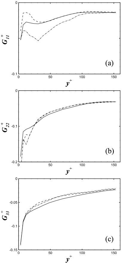
Figure 1: Diagonal components of the drift matrix, $G_{ij}$. $\tau_{p}^{+}=1$ (—) ; $\tau_{p}^{+}=5$ (– –) ; $\tau_{p}^{+}=25$ (– $\cdot$ –).

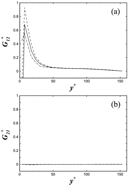
Figure 2: Non-diagonal components of the drift matrix, $G_{ij}$. $\tau_{p}^{+}=1$ (—) ; $\tau_{p}^{+}=5$ (– –) ; $\tau_{p}^{+}=25$ (– $\cdot$ –).

The results obtained for the diffusion matrix are given in the form of $B_{ij}^{2}=B_{ik}B_{jk}$ in figure 3. Contrary to the conventional modeling assumption, it is found that the diffusion term $B^{2}_{ij}$ is significantly anisotropic for $y^{+}<100$. A similar observation was previously made by Pope (2002) in a study of the stochastic Lagrangian modeling of fluid particle trajectories in a homogeneous turbulent shear flow. Besides, the results show that the components of $B_{ij}^{2}$ tend towards zero close to the wall and have a maximum located approximately at $y^{+}=25$. Consequently, according to these results, $B_{ij}^{2}$ cannot be modeled as a function of kinetic energy dissipation rate moderated by a constant since the dissipation of the kinetic energy is maximum at the wall. Concerning the inertia effect, it is observed that the values of $B_{11}^{2}$ are identical for $\tau_{p}^{+}=1\text{ and }5$ and increase when $\tau_{p}^{+}=25$. This is not the case for the components $B_{22}^{2}$ and $B_{33}^{2}$ since similar results are obtained for $\tau_{p}^{+}=5\text{ and }25$ particles while the magnitude of these components is higher for the lowest particle inertia. Regarding the non-diagonal component, the particle inertia effect is seen to only change its minimum. Using these results for the drift and diffusion matrices, the performance of the present stochastic model is examined in the next section.

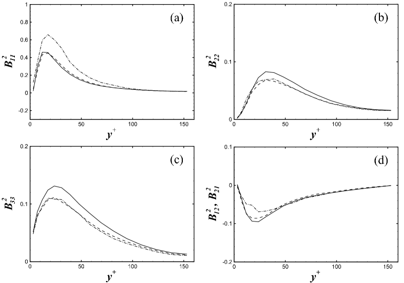
Figure 3: Components of the diffusion matrix, $B^{2}_{ij}$. $\tau_{p}^{+}=1$ (—) ; $\tau_{p}^{+}=5$ (– –) ; $\tau_{p}^{+}=25$ (– $\cdot$ –).

IV Evaluation of the stochastic models

IV.1 Presentation of the test

To assess the performance of the proposed Langevin model, a comparison between results obtained from a stochastic simulation and those extracted from the direct numerical simulation of a gas-solid channel flow has been conducted. The stochastic simulations have been carried out for three different forms of the drift vector in order to investigate the effects of this term on the predicted dispersed phase statistics. The expressions of the stochastic differential equation corresponding to these models can be put in the following compact form:

$$d\tilde{u}^{\prime}_{i}=\widetilde{G}_{ij}\tilde{u}^{\prime}_{j}dt+B_{ij}dW_{j}+D_{i}dt\,.$$ (21)

Consequently, $D_{i}=\partial\left\langle u^{\prime}_{i}u^{\prime}_{k}\right\rangle/\partial x_{k}$ gives the SDE obtained using the model proposed by Simonin et al. (1993) [Eq. (13)], $D_{i}=\partial\left\langle\tilde{u}^{\prime}_{i}v^{\prime}_{p,k}\right\rangle/\partial x_{k}$ is the second form which is derived using the proposed model for the drift vector [Eq. (14)], and $D_{i}=0$ corresponds to the third model considered. This last form is less cumbersome than the two others and does not need to know beforehand the fluid Reynolds stresses or the fluid-particle covariances. In addition, it should be noted that this model only gives the proper limit of the average of the time variation of the fluid velocity seen when $\tau_{p}\gg 1$ [see Eq. (8)].

IV.2 Stochastic simulation

For the stochastic simulation of the gas-solid flow, the mean fluid motion was calculated by means of a Reynolds-Averaged Navier-Stokes model. Closure of the Reynolds stresses is achieved using the Non Linear Eddy Viscosity Model,Speziale (1987) so that turbulence anisotropy is taken into account. In order to have a better precision in the near-wall region where the viscosity effects have to be taken into account, modifications of the standard $k-\epsilon$ model following the recommendations of Myong and Kasagi (1990) have been made. This model introduces “damping” functions that allow the transport equations of $k$ and $\epsilon$ to be valid close to the wall. A complete description of the RANS model used here is given in the work of Carlier et al. (2005). The mean fluid velocity, $\left\langle u_{1}\right\rangle^{+}$, predicted by this model is compared in figure 4 to the one obtained by DNS. Despite a slight overprediction of $\left\langle u_{1}\right\rangle^{+}$ by the RANS model in the logarithmic region, the results can be considered to be in good accordance.

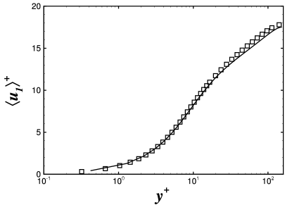
Figure 4: Mean streamwise fluid velocity, $\left\langle u_{1}\right\rangle$. DNS (—) ; RANS ($\Box$).

After the Eulerian computation of the mean fluid velocity, the stochastic Lagrangian simulations have been performed by tracking as much as $2.10^{6}$ solid particles in order to get enough statistical information in each cell of the domain to calculate the mean dispersed phase statistics. The particle characteristics as well as the equation of motion used for calculating the trajectories are identical to those of the DNS computation.
Nevertheless, contrary to the gas-solid DNS which has been conducted in a bi-periodic domain, a finite streamwise length channel has been considered for the stochastic simulation. This length has been chosen to be equal to 10 m $(\simeq 500\text{ times the channel half-width})$ in order to obtain dispersed statistics, calculated at the outlet, which are independent of the distance to the inlet.
The fluid velocity fluctuation at the particle location has been determined by integrating in time the stochastic equation [Eq. (21)] in a semi-analytical way. The stochastic part is firstly disregarded and the time increment of the velocity can be thus analytically obtained from the resulting system of coupled equations. The stochastic term increment is then estimated using an Euler scheme and added to the analytical solution. The simulations have been carried out using a time step being equal to $\tau_{p}/25$ for $\tau_{p}^{+}=5\text{ and }25$. For the $\tau_{p}^{+}=1$ particles, the time step was chosen to be $\tau_{p}/5$ in order to limit the computational cost. One should note that during these stochastic simulations, the time step is always lower or of the order of the smallest velocity timescale characterizing the present flow. This choice is also in accordance with the guideline given by Sommerfeld (2003). The values of $\widetilde{G}_{ij}$ and $B_{ij}$ have been linearly interpolated at the solid particle location from the data presented in the previous section. These coefficients being unknown at the wall, a linear extrapolation has been chosen to estimate them near the walls ($0<y^{+}<3.1$). In addition, the mean turbulent statistics, which appear in the three tested stochastic models, have been also calculated at the particle position using a linear interpolation of data extracted from the DNS computation in order to not introduce additional modeling uncertainties.

IV.3 Numerical results

The first result we present is the concentration (more precisely the number density) of solid particles across the channel width. The DNS and stochastic simulations conducted with the three different models are compared in figures 5(a-c) for $\tau^{+}_{p}=1,~{}5~{}\text{and}~{}25$ respectively. These results are interesting since they reveal that the drift model has an important effect on the particle distribution in the channel. The DNS data show that the particle concentration increases with increasing inertia (in the particle inertia range studied). This behavior can be seen as a preferential concentration effect at the macroscopic scale. Of course, it is different from the the local effect which occurs at smaller length scales.Squires and Eaton (1991); Wang and Maxey (1993); Rouson and Eaton (2001); Picciotto et al. (2005)
The comparison with the stochastic simulation shows also that the model of the drift vector proposed by Simonin et al. (1993) [Eq. (21) with $D_{i}=\partial\left\langle u^{\prime}_{i}u^{\prime}_{k}\right\rangle/\partial x_{k}$] is not able to reproduce the accumulation of the larger particles in the low turbulent intensity regions. The concentration profiles remain quite uniform whatever the particle inertia. It seems that the presence in the SDE of the term $D_{i}=\partial\left\langle u^{\prime}_{i}u^{\prime}_{k}\right\rangle/\partial x_{k}$ (which does not vary as a function of particle inertia) prevents the accumulation. On contrary, the model with $D_{i}=0$ produces a segregation of the particles in the near-wall region even for the lowest particle inertia. This is in contradiction with the law of conservation of mass since these particles, which can be assimilated to fluid particle tracers, have to approximately be uniformly distributed.Thomson (1987) This non-physical behavior, which is called spurious drift effect, was observed by Wilson et al. (1981) and MacInnes and Bracco (1992) in stochastic Lagrangian simulations of tracer particles in non-homogeneous turbulent flow. In fact, it is due to an inconsistency between the stochastic Lagrangian model and the Navier-Stokes equations which causes a misrepresentation of the averaged time derivative of the fluctuating fluid particle velocity. A more detailed presentation of this effect can be found in Pope (1987), Thomson (1987), Guingo and Minier (2008), and references within. Despite this major problem for low particle inertia, this stochastic model predicts reasonably well the concentration of the $\tau_{p}^{+}=25$ particles. This confirms that this latter model should be more appropriate to estimate the fluid velocity seen by large particle inertia. Finally, it is noted that the results obtained with the present model for $\tau_{p}^{+}=1\text{ and }25$ are in good accordance with the DNS data while important discrepancies are observed for $\tau_{p}^{+}=5$ when $y^{+}<2$. Nevertheless, the main point is that this model reproduces qualitatively quite well the effect of inertia on the particle concentration. There is no spurious drift effect for low inertia and an increase of the concentration in the near-wall region is noted for the higher particle inertia. This result is of importance since the correct prediction of particle flux in wall-bounded turbulent flows is decisive when studying the complex process of particle deposition.

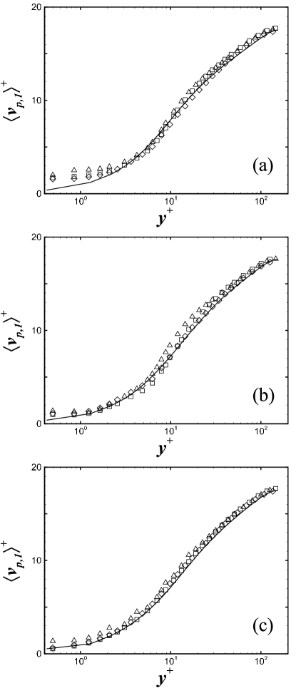
Figure 6: Mean streamwise particle velocity, $\left\langle v_{p,1}\right\rangle$, for $\tau_{p}^{+}=1$ (a), $\tau_{p}^{+}=5$ (b), and $\tau_{p}^{+}=25$ (c). DNS: — . Stochastic simulation with $D_{i}=\partial\left\langle\tilde{u}^{\prime}_{i}v^{\prime}_{p,k}\right\rangle/\partial x_{k}$ ($\Box$) ; $D_{i}=\partial\left\langle u^{\prime}_{i}u^{\prime}_{k}\right\rangle/\partial x_{k}$ ($\triangle$) ; $D_{i}=0$ ($\Diamond$).

The first order statistical moment of the particle velocity is plotted in figures 6(a-c). From Fig. 6(a), it is seen that the mean velocity of the smallest particle inertia studied is quite well predicted across the channel by the different models of the drift vector. Nevertheless, this velocity is overestimated in the viscous sublayer for $y^{+}<2$. The observed discrepancy can be reasonably attributed to the combination of two approximations. The first one concerns the local homogeneity assumption made to derive the parameters of the stochastic which does not hold in this region. The second one is the linear extrapolation used to estimate these parameters at the particle location. These remarks should be kept in mind throughout the presentation of the results. In the buffer and logarithmic regions, the present model as well as the one of Simonin et al. (1993) give similar results which are slightly greater than those of the DNS. This is due to the fact that the RANS model slightly overestimates the mean fluid velocity given by the DNS. Concerning the results obtained with the third model tested, i.e. Eq. (21) with $D_{i}=0$, we note that they are similar to those of the two other models except in the buffer region where the mean particle is lower. It is believed that this interesting difference is due to the fact that this model is not compatible with the transport equation of the drift velocity in the limit of low particle inertia. This incompatibility certainly gives rise to a wrong estimation of the drift velocity which should be quite low for this kind of particles. Since the mean particle velocity is lower than expected, it can concluded that this model generates fluctuations of the fluid velocity whose average is negative.
The mean velocity of the $\tau_{p}^{+}=5$ particles is shown in Fig. 6(b). Firstly, the present model and the one with $D_{i}=0$ give identical results. The mean particle velocity is also slightly overestimated in the buffer and logarithmic regions. Nonetheless, the discrepancy observed for the smaller particles in the near-wall region is attenuated. This is certainly due to the less important sensitivity of the $\tau_{p}^{+}=5$ particles to the fluctuating fluid velocity. Secondly, it is noticed that the model of Simonin et al. (1993) causes a too high particle velocity in the buffer region. The incompatibility of this model with the transport equation of the drift velocity in the limit of large particle inertia can be invoked. Nevertheless, this explanation has to be taken with caution since one could argue that $\tau_{p}^{+}=5$ particles do not belong to the category of large particles. At this stage of the study, no clear conclusion can be drawn.
The mean velocity of $\tau_{p}^{+}=25$ particles is plotted in Fig. 6(c), the three models give approximately the same results in the buffer and logarithmic regions. The predicted velocity is once more slightly higher than the one extracted from the DNS. In the viscous sublayer, this overprediction is also observed for the model of Simonin et al. (1993) while the results with the two other models are in a good accordance with the DNS.

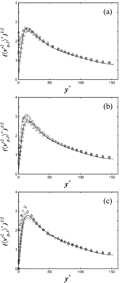
Figure 7: Root mean square of the streamwise particle velocity, $(\left\langle v^{\prime 2}_{p,1}\right\rangle)^{1/2}$, for $\tau_{p}^{+}=1$ (a), $\tau_{p}^{+}=5$ (b), and $\tau_{p}^{+}=25$ (c). DNS: — . Stochastic simulation with $D_{i}=\partial\left\langle\tilde{u}^{\prime}_{i}v^{\prime}_{p,k}\right\rangle/\partial x_{k}$ ($\Box$) ; $D_{i}=\partial\left\langle u^{\prime}_{i}u^{\prime}_{k}\right\rangle/\partial x_{k}$ ($\triangle$) ; $D_{i}=0$ ($\Diamond$).

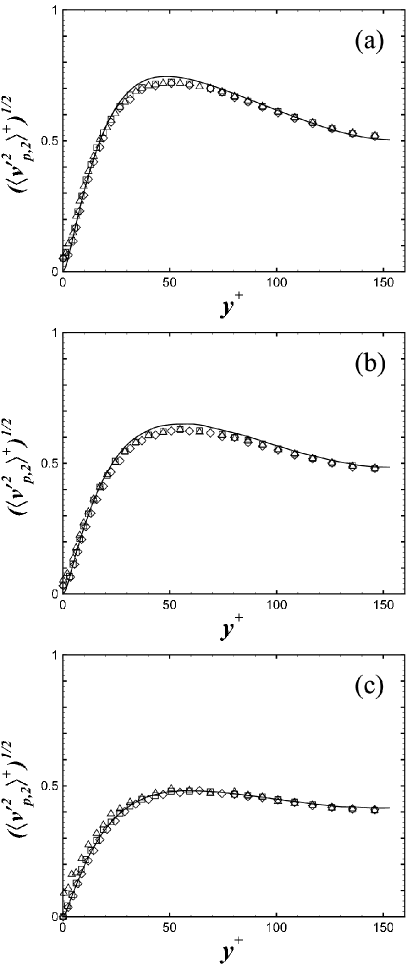
Figure 8: Root mean square of the wall-normal particle velocity, $(\left\langle v^{\prime 2}_{p,2}\right\rangle)^{1/2}$, for $\tau_{p}^{+}=1$ (a), $\tau_{p}^{+}=5$ (b), and $\tau_{p}^{+}=25$ (c). DNS: — . Stochastic simulation with $D_{i}=\partial\left\langle\tilde{u}^{\prime}_{i}v^{\prime}_{p,k}\right\rangle/\partial x_{k}$ ($\Box$) ; $D_{i}=\partial\left\langle u^{\prime}_{i}u^{\prime}_{k}\right\rangle/\partial x_{k}$ ($\triangle$) ; $D_{i}=0$ ($\Diamond$).

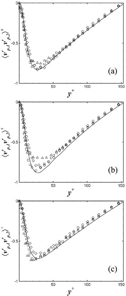
Figure 9: Particle kinetic shear stress, $\left\langle v^{\prime}_{p,1}v^{\prime}_{p,2}\right\rangle$, for $\tau_{p}^{+}=1$ (a), $\tau_{p}^{+}=5$ (b), and $\tau_{p}^{+}=25$ (c). DNS: — . Stochastic simulation with $D_{i}=\partial\left\langle\tilde{u}^{\prime}_{i}v^{\prime}_{p,k}\right\rangle/\partial x_{k}$ ($\Box$) ; $D_{i}=\partial\left\langle u^{\prime}_{i}u^{\prime}_{k}\right\rangle/\partial x_{k}$ ($\triangle$) ; $D_{i}=0$ ($\Diamond$).

In order to better understand the influence of this three different stochastic models, the particle velocity root mean square (rms) has also been computed. The results obtained are shown in figures 7-9. The estimated values of the streamwise particle velocity rms for the $\tau_{p}^{+}=1$ particles [Fig. 7(a)] are seen to be in very good accordance with the DNS results. For the $\tau_{p}^{+}=5$ particles [Fig. 7(b)], some differences are noted for $y^{+}<30$. Surprisingly, better results are obtained with the simplest model studied [i.e. Eq. (21) with $D_{i}=0$]. The two other models overestimate the streamwise particle velocity rms. The difference is roughly of the order of 5%. The results obtained for $\tau_{p}^{+}=25$ [Fig. 7(c)] show that the present model and the one with $D_{i}=0$ predict accurately this particle velocity statistical moment. Some important discrepancies are noticed with the model by Simonin et al. (1993) for $y^{+}<15$. Concerning the wall-normal component plotted in figure 8, it can be seen that the accordance with the DNS results is very good whatever the model used. The predicted values are slightly lower than those given by the DNS for $\tau_{p}^{+}=1\text{ and }5$, however, this difference is not significant. The inertia filtering effect is consequently well reproduced by the stochastic models. For sake of conciseness and due to its strong qualitative similarity with the wall-normal component, the spanwise velocity rms is not shown. The non-diagonal component of the particle velocity rms is presented in Fig. 9. More important differences are observed for this component than for the others. Concerning the smallest particle inertia, the three models are in good agreement with the DNS data. For higher inertia, the results obtained from these models diverge for $10<y^{+}<50$. In this region, the model by Simonin et al. (1993) underestimates the magnitude of the minimum of particle kinetic shear stress $\left\langle v^{\prime}_{p,1}v^{\prime}_{p,2}\right\rangle$. This trend is also obtained with the two other models, however, the difference is less. It should be also noted that the magnitude of $\left\langle v^{\prime}_{p,1}v^{\prime}_{p,2}\right\rangle$ given by DNS is higher than that of the three stochastic models for $y^{+}>50$. A possible reason for this disagreement is that the wall-shear velocity used to normalized the quantities shown is not perfectly identical in the DNS and stochastic simulations. Finally, it can be remarked that the differences noticed previously are less for the $\tau_{p}^{+}=25$ particle except for $y^{+}>50$ where the underestimation of the magnitude particle kinetic shear stress is of the same order.

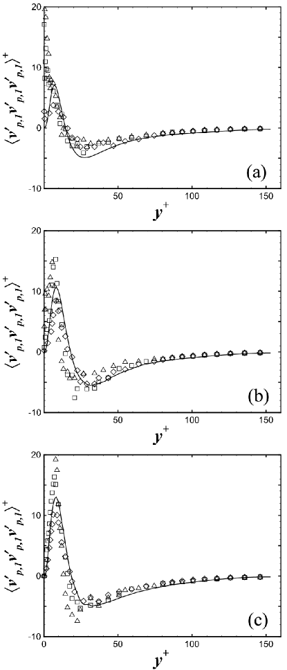
Figure 10: Triple particle velocity correlation, $\left\langle v^{\prime}_{p,1}v^{\prime}_{p,1}v^{\prime}_{p,1}\right\rangle$, for $\tau_{p}^{+}=1$ (a), $\tau_{p}^{+}=5$ (b), and $\tau_{p}^{+}=25$ (c). DNS: — . Stochastic simulation with $D_{i}=\partial\left\langle\tilde{u}^{\prime}_{i}v^{\prime}_{p,k}\right\rangle/\partial x_{k}$ ($\Box$) ; $D_{i}=\partial\left\langle u^{\prime}_{i}u^{\prime}_{k}\right\rangle/\partial x_{k}$ ($\triangle$) ; $D_{i}=0$ ($\Diamond$).

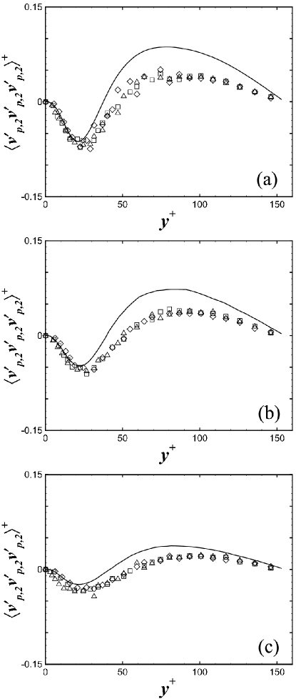
Figure 11: Triple particle velocity correlation, $\left\langle v^{\prime}_{p,2}v^{\prime}_{p,2}v^{\prime}_{p,2}\right\rangle$, for $\tau_{p}^{+}=1$ (a), $\tau_{p}^{+}=5$ (b), and $\tau_{p}^{+}=25$ (c). DNS: — . Stochastic simulation with $D_{i}=\partial\left\langle\tilde{u}^{\prime}_{i}v^{\prime}_{p,k}\right\rangle/\partial x_{k}$ ($\Box$) ; $D_{i}=\partial\left\langle u^{\prime}_{i}u^{\prime}_{k}\right\rangle/\partial x_{k}$ ($\triangle$) ; $D_{i}=0$ ($\Diamond$).

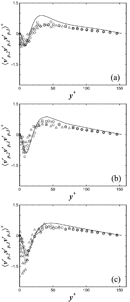
Figure 12: Triple particle velocity correlation, $\left\langle v^{\prime}_{p,2}v^{\prime}_{p,1}v^{\prime}_{p,1}\right\rangle$, for $\tau_{p}^{+}=1$ (a), $\tau_{p}^{+}=5$ (b), and $\tau_{p}^{+}=25$ (c). DNS: — . Stochastic simulation with $D_{i}=\partial\left\langle\tilde{u}^{\prime}_{i}v^{\prime}_{p,k}\right\rangle/\partial x_{k}$ ($\Box$) ; $D_{i}=\partial\left\langle u^{\prime}_{i}u^{\prime}_{k}\right\rangle/\partial x_{k}$ ($\triangle$) ; $D_{i}=0$ ($\Diamond$).

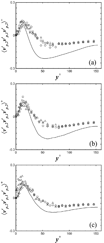
Figure 13: Triple particle velocity correlation, $\left\langle v^{\prime}_{p,2}v^{\prime}_{p,1}v^{\prime}_{p,2}\right\rangle$, for $\tau_{p}^{+}=1$ (a), $\tau_{p}^{+}=5$ (b), and $\tau_{p}^{+}=25$ (c). DNS: — . Stochastic simulation with $D_{i}=\partial\left\langle\tilde{u}^{\prime}_{i}v^{\prime}_{p,k}\right\rangle/\partial x_{k}$ ($\Box$) ; $D_{i}=\partial\left\langle u^{\prime}_{i}u^{\prime}_{k}\right\rangle/\partial x_{k}$ ($\triangle$) ; $D_{i}=0$ ($\Diamond$).

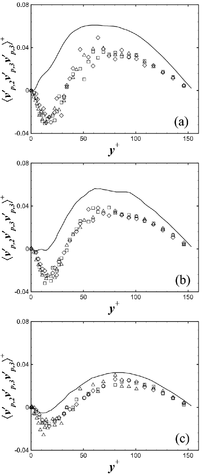
Figure 14: Triple particle velocity correlation, $\left\langle v^{\prime}_{p,2}v^{\prime}_{p,3}v^{\prime}_{p,3}\right\rangle$, for $\tau_{p}^{+}=1$ (a), $\tau_{p}^{+}=5$ (b), and $\tau_{p}^{+}=25$ (c). DNS: — . Stochastic simulation with $D_{i}=\partial\left\langle\tilde{u}^{\prime}_{i}v^{\prime}_{p,k}\right\rangle/\partial x_{k}$ ($\Box$) ; $D_{i}=\partial\left\langle u^{\prime}_{i}u^{\prime}_{k}\right\rangle/\partial x_{k}$ ($\triangle$) ; $D_{i}=0$ ($\Diamond$).

To complete this comparison of the particle velocity statistics, the prediction of a higher statical moment (the triple particle velocity correlations $\left\langle v^{\prime}_{p,i}v^{\prime}_{p,j}v^{\prime}_{p,k}\right\rangle$) has been also investigated. This will give an idea of the capability of stochastic modeling. The agreement with the DNS data is not expected to be as good as for the other statistical moments shown due to the assumptions made for the derivation of the parameters of the stochastic models. The streamwise triple particle velocity correlation is plotted in figure 10. Surprisingly, the three stochastic models are seen to be able to predict very well this correlation for $y^{+}>30$ and whatever the particle inertia. Moreover, the models well estimate the inertia effect since the obtained maximum of this correlation (located at $y^{+}\simeq 10$) increases with increasing inertia. Nonetheless, the magnitude of this maximum is not well predicted since the present model as well as the one by Simonin et al. (1993) clearly overestimate it while an underestimation is noted for the model with $D_{i}=0$. From figure 12, it can be observed that $\left\langle v^{\prime}_{p,2}v^{\prime}_{p,1}v^{\prime}_{p,1}\right\rangle$ is also quite well predicted by the present model and the one with $D_{i}=0$ across the channel and whatever the particle inertia. Concerning the model of Simonin et al. (1993), more important discrepancies arise for $y^{+}<20$ and $\tau_{p}^{+}=5\text{ and }25$. For the correlations $\left\langle v^{\prime}_{p,2}v^{\prime}_{p,2}v^{\prime}_{p,2}\right\rangle$ and $\left\langle v^{\prime}_{p,2}v^{\prime}_{p,1}v^{\prime}_{p,2}\right\rangle$, shown in figures 11 and 13, a similar trend is noted. First, the results given by the three stochastic models are almost identical. Secondly, the agreement with the DNS data is very good when $y^{+}<20$ whereas the magnitude of these two correlations is significantly underestimated in the rest of the channel. The last non-zero correlation computed is $\left\langle v^{\prime}_{p,2}v^{\prime}_{p,3}v^{\prime}_{p,3}\right\rangle$ (Fig. 14). There are major differences between the DNS and stochastic simulations. The predicted correlation is generally smaller than the one extracted from the DNS. In addition, for $y^{+}<40$ and the smallest particle inertia, the wrong sign of $\left\langle v^{\prime}_{p,2}v^{\prime}_{p,3}v^{\prime}_{p,3}\right\rangle$ is given by the stochastic models. Nonetheless, the results obtained with these models are in a good qualitative agreement for $y^{+}>40$, and the inertia effect, which causes a decrease of this correlation, is well estimated.

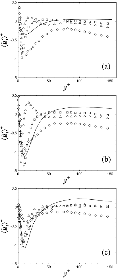
Figure 15: Streamwise drift velocity, $\left\langle\tilde{u}^{\prime}_{1}\right\rangle$, for $\tau_{p}^{+}=1$ (a), $\tau_{p}^{+}=5$ (b), and $\tau_{p}^{+}=25$ (c). DNS: — . Stochastic simulation with $D_{i}=\partial\left\langle\tilde{u}^{\prime}_{i}v^{\prime}_{p,k}\right\rangle/\partial x_{k}$ ($\Box$) ; $D_{i}=\partial\left\langle u^{\prime}_{i}u^{\prime}_{k}\right\rangle/\partial x_{k}$ ($\triangle$) ; $D_{i}=0$ ($\Diamond$).

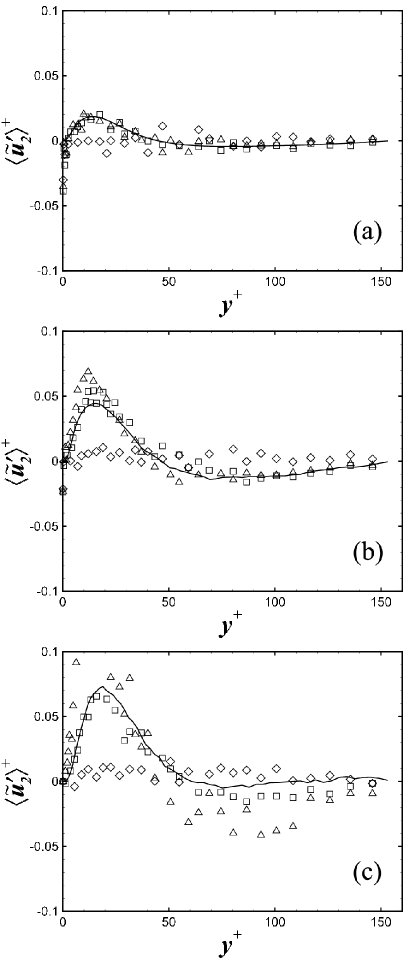
Figure 16: Wall-normal drift velocity, $\left\langle\tilde{u}^{\prime}_{2}\right\rangle$, for $\tau_{p}^{+}=1$ (a), $\tau_{p}^{+}=5$ (b), and $\tau_{p}^{+}=25$ (c). DNS: — . Stochastic simulation with $D_{i}=\partial\left\langle\tilde{u}^{\prime}_{i}v^{\prime}_{p,k}\right\rangle/\partial x_{k}$ ($\Box$) ; $D_{i}=\partial\left\langle u^{\prime}_{i}u^{\prime}_{k}\right\rangle/\partial x_{k}$ ($\triangle$) ; $D_{i}=0$ ($\Diamond$).

The second part of this comparison between the DNS and stochastic simulations is devoted to the statistics of the fluid seen velocity. The first statistical moment studied is the drift velocity $\left\langle\tilde{u}^{\prime}_{i}\right\rangle$. In figures 15 and 16, the streamwise and wall-normal components are presented. A better prediction of the drift velocity from the present model is expected since it has been previously shown that it is the only model of the three considered which is compatible with the transport equation of this velocity in the limits of low and high particle inertia. From the results obtained for the streamwise component, it can be seen that the three models are unable to correctly estimate it for the $\tau_{p}^{+}=1$ particles when $y^{+}<40$. The present model and the one of Simonin et al. (1993) predict quite correctly $\left\langle\tilde{u}^{\prime}_{1}\right\rangle$ in the rest of the channel while significant difference with the DNS data are still noted using the model with $D_{i}=0$. This is in line with the fact that this latter model is not compatible with the transport equation of the drift velocity when $\tau_{p}^{+}\rightarrow 0$. As shown in the first part of this study, the two other models become identical in this limit. Nevertheless, there are some differences. This is due to the value of the particle inertia studied which is not enough low to observe the convergence of these two models. It is confirmed by the DNS data since the drift velocity of the $\tau_{p}^{+}=1$ particles is non-null while this velocity has to vanish when $\tau_{p}^{+}\rightarrow 0$. From figure 15(b), it is apparent that the model with $D_{i}=0$ better predicts the drift velocity for this kind of particles, however, there are important inconsistencies in a large part of the channel. The results given by the present model are in satisfactory agreement with the DNS data, whereas important qualitative and quantitative discrepancies are noted for the model by Simonin et al. (1993) when $10<y^{+}<30$. In the case of the highest particle inertia, this latter model and the present one give surprisingly similar results which are in acceptable agreement with the DNS data while the predictions by the simple model with $D_{i}=0$ are poor. It could have been expected that this latter model would lead to better results for these particles. Nonetheless, the inertia of the particle studied is not enough high to show that the present model and the one with $D_{i}=0$ should predict the drift velocity more accurately than the model by Simonin et al. (1993). The capability of the three models can be better distinguished from the results of the wall-normal component of the drift velocity. The stochastic model with $D_{i}=0$ predicts a null drift velocity whatever the distance to the wall and the particle inertia. It is in complete disagreement with the DNS data. The results obtained with the model by Simonin et al. (1993) are in satisfactory accordance. Nevertheless, important discrepancies begin to arise as the particle inertia increases. Contrary to these two models, the expression proposed to estimate the drift vector of the stochastic equation leads to a good estimation of this drift velocity whatever the particle inertia. These observations can explain the predictions of the particle concentration by the three models making use of simple physical considerations. The wall-normal drift velocity given by the stochastic model with $D_{i}=0$ is null. It has been also shown that this model predicts an increase of particle concentration in the near-wall region whatever the particle inertia. This non-physical increase in the case of the lowest particle inertia is induced by the fact that there is no mean force to counteract the accumulation of the particles in low-turbulence regions (the so-called turbophoresis effectCaporaloni et al. (1975); Reeks (1983)). To explain the uniform concentration obtained with the model by Simonin et al. (1993) whereas an increase should be observed near the wall in the case of the $\tau_{p}^{+}=5\text{ and }25$ particles, similar considerations can be put forward. The predicted drift velocity given by this model, which is higher than that of the present model, is certainly too high to make possible the accumulation of these particles.

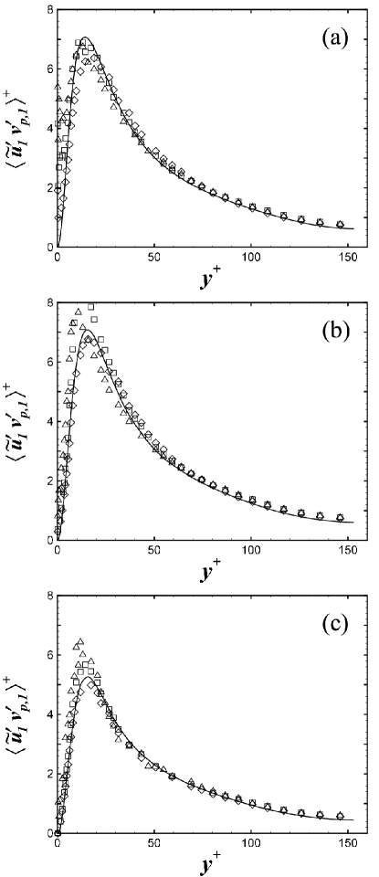
Figure 17: Diagonal component of the fluid-particle covariance tensor, $\left\langle\tilde{u}^{\prime}_{1}v^{\prime}_{p,1}\right\rangle$, for $\tau_{p}^{+}=1$ (a), $\tau_{p}^{+}=5$ (b), and $\tau_{p}^{+}=25$ (c). DNS: — . Stochastic simulation with $D_{i}=\partial\left\langle\tilde{u}^{\prime}_{i}v^{\prime}_{p,k}\right\rangle/\partial x_{k}$ ($\Box$) ; $D_{i}=\partial\left\langle u^{\prime}_{i}u^{\prime}_{k}\right\rangle/\partial x_{k}$ ($\triangle$) ; $D_{i}=0$ ($\Diamond$).

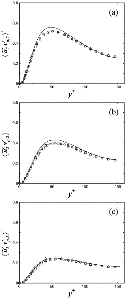
Figure 18: Diagonal component of the fluid-particle covariance tensor, $\left\langle\tilde{u}^{\prime}_{2}v^{\prime}_{p,2}\right\rangle$, for $\tau_{p}^{+}=1$ (a), $\tau_{p}^{+}=5$ (b), and $\tau_{p}^{+}=25$ (c). DNS: — . Stochastic simulation with $D_{i}=\partial\left\langle\tilde{u}^{\prime}_{i}v^{\prime}_{p,k}\right\rangle/\partial x_{k}$ ($\Box$) ; $D_{i}=\partial\left\langle u^{\prime}_{i}u^{\prime}_{k}\right\rangle/\partial x_{k}$ ($\triangle$) ; $D_{i}=0$ ($\Diamond$).

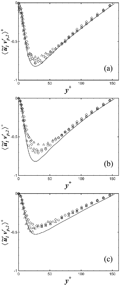
Figure 19: Non-diagonal component of the fluid-particle covariance tensor, $\left\langle\tilde{u}^{\prime}_{1}v^{\prime}_{p,2}\right\rangle$, for $\tau_{p}^{+}=1$ (a), $\tau_{p}^{+}=5$ (b), and $\tau_{p}^{+}=25$ (c). DNS: — . Stochastic simulation with $D_{i}=\partial\left\langle\tilde{u}^{\prime}_{i}v^{\prime}_{p,k}\right\rangle/\partial x_{k}$ ($\Box$) ; $D_{i}=\partial\left\langle u^{\prime}_{i}u^{\prime}_{k}\right\rangle/\partial x_{k}$ ($\triangle$) ; $D_{i}=0$ ($\Diamond$).

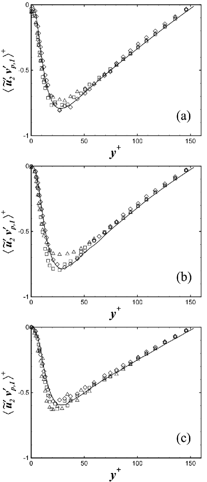
Figure 20: Non-diagonal component of the fluid-particle covariance tensor, $\left\langle\tilde{u}^{\prime}_{2}v^{\prime}_{p,1}\right\rangle$, for $\tau_{p}^{+}=1$ (a), $\tau_{p}^{+}=5$ (b), and $\tau_{p}^{+}=25$ (c). DNS: — . Stochastic simulation with $D_{i}=\partial\left\langle\tilde{u}^{\prime}_{i}v^{\prime}_{p,k}\right\rangle/\partial x_{k}$ ($\Box$) ; $D_{i}=\partial\left\langle u^{\prime}_{i}u^{\prime}_{k}\right\rangle/\partial x_{k}$ ($\triangle$) ; $D_{i}=0$ ($\Diamond$).

The last statistical moment considered in this evaluation of the proposed stochastic model is the fluid seen-particle velocity correlations $\left\langle\tilde{u}^{\prime}_{i}v^{\prime}_{p,j}\right\rangle$. Concerning the diagonal components presented in Figs. 17 and 18, the agreement of the stochastic simulations with the DNS data exhibits the same trends as for the particle velocity rms. The three models almost perfectly reproduce the inertia effect on the wall-normal and spanwise components. It should be noted that due to the strong similarity between these two components, only the results obtained for $\left\langle\tilde{u}^{\prime}_{2}v^{\prime}_{p,2}\right\rangle$ are shown (see Fig. 18). From figure 17, it is noted that the streamwise component is in good accordance with the DNS data in the case of the smaller particle inertia. Differences appear for higher particle inertia near the location of the maximum of $\left\langle\tilde{u}^{\prime}_{1}v^{\prime}_{p,1}\right\rangle$ ($10<y^{+}<20$). As observed for the particle velocity rms, the present model as well as the one by Simonin et al. (1993) lead to an overprediction of the streamwise component while a better agreement is obtained with the third model [Eq. (21) with $D_{i}=0$]. Due to the asymmetry of the fluid seen-particle velocity correlations, the two non-diagonal components are presented in figures 19 and 20. The evolution of $\left\langle\tilde{u}^{\prime}_{1}v^{\prime}_{p,2}\right\rangle$ as a function of the particle inertia is well reproduced. Nonetheless, the stochastic models generally underestimate the DNS results. A better agreement is obtained for the other non-diagonal component. As noted for the majority of the statistics presented in this study, the model by Simonin et al. (1993) provides an acceptable but less accurate prediction.

V Conclusion

We present in this study a stochastic model for estimating the fluid velocity experienced by small solid particles in a non-homogeneous turbulent flow. In the first part, a new stochastic model which is compatible with the limits of the transport equation of the drift velocity for low and high particle inertia has been derived. From this compatibility criterion, it has also been shown that some previously proposed stochastic models should not be able to reflect accurately the inertia effect on the fluid velocity seen by high inertia particles.

In the second part of this study, the accuracy of the present stochastic equation has been evaluated. Since no models exist to determine the drift and diffusion parameters, appearing in the SDE, for non-homogeneous turbulence, they have been deduced from a method similar to the one proposed by Pope (2002). The obtained results show that the drift and diffusion matrices are highly space-dependent and anisotropic. Using these values, stochastic simulations of a gas-solid channel flow have been conducted and compared to DNS. The stochastically predicted data have been also compared to those obtained with the model proposed by Simonin et al. (1993) and to a simpler one. Using the compatibility criterion presented in the first part, the former model should not be able to reproduce the dynamics of high particle inertia while the latter should not be able to reproduce it for small particle inertia.
The three models considered are able to predict with a good accuracy the first and second order statistical moments of the particle and fluid seen velocities. Surprisingly, a good accordance has been also noticed for the triple particle velocity correlations. This accordance is mainly qualitative. Nevertheless, some components have been seen to be well predicted quantitatively. This clearly demonstrates the capability of Langevin-type models to predict accurately and efficiently the interactions between inertial particles and turbulence.
The accuracy of the results obtained with these three different models diverges principally for the particle concentration and the drift velocity. As stated before, a good estimation of these quantities is primordial to correctly predict the important process of particle deposition. It has been seen that the model proposed by Simonin et al. (1993) is not able to predict the increase near the wall of the concentration of moderate and high particle inertia. On contrary, the simpler model predicts this increase even for the smaller particle inertia whereas the concentration should be almost uniform. This clearly shows that this model suffers from a spurious drift effect. The new proposed model is the only one which succeeds in predicting the good evolution of the particle concentration for the range of particle inertia studied. This naturally leads us to consider that it is a good candidate to estimate the turbulence seen by inertial particles. In the present paper, we test the proposed model using DNS data such as for the fluid-particle covariances in order to not introduce supplementary modeling uncertainties. These data are generally not known beforehand. Nonetheless, numerical strategies related to RANS-Lagrangian methods can help to overcome this difficulty. For instance, one such method can be found in Peirano et al. (2006), which calculates the fluid-particle covariances on the basis of the statistics of a large number of particles. Thus, the model is more computationally demanding than Simonin’s method, but it is hoped that the benefit of better results outweighs the extra cost.
Another possible way to bypass this difficulty would be to directly model the fluid-particle covariances. The simplest existing model is based on the theory developed by Tchen (1947) and Hinze (1975) [see Simonin et al. (1993)]. Attention must be paid to the properties of the carrier fluid flow studied since this model was initially developed for isotropic and stationary turbulence under restrictive assumptions. A more sophisticated approach was recently proposed by Zaichik et al. (2004). Although their model was developed for quasi-homogeneous anistropic turbulence, quite accurate predictions of the fluid-particle covariances were obtain for a gas-solid non-homogeneous flow.Arcen et al. (2008) Moreover, the union of these models with the proposed stochastic equation is consistent since both depend on the same set of quantities, i.e. the decorrelation time scales and second order statistical moment of the fluid velocity seen by particles.

We would like to emphasize that the model proposed belongs to a particular class of stochastic models. Many other models could certainly reproduce more accurately the interactions between inertial particles and turbulence. Nonetheless, the difficulty is to find a model which is a good compromise between complexity and physical accuracy. Besides, the challenge lies also in the specification of the model parameters. One could propose a model which is theoretically able to reproduce the different physical aspects of gas-solid flows with high fidelity, but if its parameters cannot be estimated accurately, the model will probably be less satisfactory than a simpler model whose parameters can be found precisely. One part of the physics is in the functional form of the model, the other part is in its parameters.

Finally, it should be noted that Lagrangian stochastic methods can also be considered for predicting the motion of gas bubbles in a liquid. Nevertheless, deformation, coalescence and break-up can significantly modify bubbles shape, and consequently, alter the interactions of each bubbles with turbulence. This makes the use of a stochastic model more complex since its parameters, which are not well known, should be correctly modified during the bubble tracking. In addition, the use of the point-force approximation could become ambiguous when bubble coalescence is strong. However, if we restrict ourselves to small non-deformable bubbles and neglect break-up and coalescence, a Lagrangian stochastic method can be retained. As for solid particles, the difficulty will be to properly estimate the parameters of the stochastic model.

Figure 5: Particle concentration, $C_{p}$, for $\tau_{p}^{+}=1$ (a), $\tau_{p}^{+}=5$ (b), and $\tau_{p}^{+}=25$ (c). DNS: — . Stochastic simulation with $D_{i}=\partial\left\langle\tilde{u}^{\prime}_{i}v^{\prime}_{p,k}\right\rangle/\partial x_{k}$ ($\Box$) ; $D_{i}=\partial\left\langle u^{\prime}_{i}u^{\prime}_{k}\right\rangle/\partial x_{k}$ ($\triangle$) ; $D_{i}=0$ ($\Diamond$).

References

- Maxey and Riley (1983) M. Maxey and J. Riley, “Equation of motion for small rigid sphere in non uniform flow,” Phys. Fluids 26, 883 (1983).
- Reeks (1977) M. W. Reeks, “On the dispersion of small particles suspended in an isotropic turbulence,” J. Fluid Mech. 83, 529 (1977).
- McLaughlin (1989) J. B. McLaughlin, “Aerosol particle deposition in numerically simulated channel flow,” Phys. Fluids 1, 1211 (1989).
- Rouson and Eaton (2001) D. W. I. Rouson and J. K. Eaton, “On the preferential concentration of solid particles in turbulent channel flow,” J. Fluid Mech. 428, 149 (2001).
- Ferrante and Elghobashi (2003) A. Ferrante and S. Elghobashi, “On the physical mechanims of two-way coupling in particle-laden isotropic turbulence,” Phys. Fluids 15, 315 (2003).
- Marchioli et al. (2008a) C. Marchioli, M. V. Salvetti, and A. Soldati, “Some issues concerning large-eddy simulation of inertial particle dispersion in turbulent bounded flows,” Phys. Fluids 20, 040603 (2008a).
- Mashayek and Pandya (2003) F. Mashayek and R. V. R. Pandya, “Analytical description of particle/droplet-laden turbulent flows,” Prog. Energy Combust. Sci. 29, 329 (2003).
- Simonin et al. (1993) O. Simonin, E. Deutsch, and J. P. Minier, “Eulerian prediction of fluid-particle correlated motion in turbulent two-phase flows,” Applied Scientific Research 51, 275 (1993).
- Oesterlé and Zaichik (2004) B. Oesterlé and L. I. Zaichik, “On lagrangian time scales and particle dispersion modeling in equilibrium shear flows,” Phys. Fluids 16, 3374 (2004).
- Iliopoulos and Hanratty (2004) I. Iliopoulos and T. J. Hanratty, “A non-gaussian stochastic model to describe passive tracer dispersion and its comparison to a direct numerical simulation,” Phys. Fluids 16, 3006 (2004).
- Reeks (2005) M. W. Reeks, “On probability density function equations for particle dispersion in a uniform shear flow,” J. Fluid Mech. 522, 263 (2005).
- Pialat et al. (2007) X. Pialat, O. Simonin, and P. Villedieu, “A hybrid Eulerian-Lagrangian method to simulate the dispersed phase in turbulent gas-particle flows,” Int. J. of Multiphase Flow 33, 766 (2007).
- Dehbi (2008) A. Dehbi, “Turbulent particle dispersion in arbitrary wall-bounded geometries: A coupled CFD-Langevin-equation based approach,” Int. J. of Multiphase Flow 34, 819 (2008).
- Gardiner (1997) C. W. Gardiner, Handbook of Stochastic Methods for Physics, Chemistry and the Natural Sciences, Springer-Verlag, Berlin, 2nd edition (1997).
- Minier and Peirano (2001) J. P. Minier and E. Peirano, “The PDF approach to turbulent polydispersed two-phase flows,” Physics Reports 352, 1 (2001).
- Csanady (1963) G. T. Csanady, “Turbulent diffusion of heavy particles in the atmosphere,” J. Atmos. Sci. 20, 201 (1963).
- Pope (1983) S. B. Pope, “A Lagrangian two-time probability density function equation for inhomogeneous turbulent flows,” Phys. Fluids 26, 3448 (1983).
- Simonin (2000) O. Simonin, “Statistical and continuum modelling of turbulent reactive particulate flows,” (2000), lecture series 2000-06. von Karman Institute for Fluid Dynamics, Rhode-St-Genèse, Belgium.
- Pandya and Mashayek (2003) R. V. R. Pandya and F. Mashayek, “Non-isothermal dispersed phase of particles in turbulent flow,” J. Fluid Mech. 475, 205 (2003).
- Bocksell and Loth (2006) T. L. Bocksell and E. Loth, “Stochastic modeling of particle diffusion in a turbulent boundary layer,” Int. J. of Multiphase Flow 32, 1234 (2006).
- Pope (1987) S. B. Pope, “Consistency conditions for random-walk models of turbulent dispersion,” Phys. Fluids 30, 2374 (1987).
- Pope (2002) S. B. Pope, “Stochastic Lagrangian models of velocity in homogeneous turbulent flow,” Phys. Fluids 14, 1696 (2002).
- Iliopoulos and Hanratty (1999) I. Iliopoulos and T. J. Hanratty, “Turbulent dispersion in a non-homogeneous field,” J. Fluid Mech. 392, 45 (1999).
- Iliopoulos et al. (2003) I. Iliopoulos, Y. Mito, and T. J. Hanratty, “A stochastic model for solid particle dispersion in a nonhomogeneous turbulent field,” Int. J. of Multiphase Flow 29, 375 (2003).
- Thomson (1987) D. J. Thomson, “Criteria for the selection of stochastic models of particle trajectories in turbulent flows,” J. Fluid Mech. 180, 529 (1987).
- Wilson et al. (1981) J. D. Wilson, G. W. Thurtell, and G. E. Kidd, “Numerical simulation of particle trajectories in inhomogeneous turbulence, II: Systems with variable turbulent velocity scale,” Boundary-Layer Meteorol. 21, 423 (1981).
- Thomson (1984) D. J. Thomson, “Random walk modelling of diffusion in inhomogeneous turbulence,” Quart. J. R. Meteor. Soc. 110, 1107 (1984).
- Durbin (1983) P. A. Durbin, “Stochastic differential equations and turbulent dispersion,” (1983), NASA Reference Publication 1103. Available from the Nasa Technical Reports Server.
- Walpot et al. (2007) R. J. E. Walpot, C. W. M. van der Geld, and J. G. M. Kuerten, “Determination of the coefficients of Langevin models in inhomogeneous turbulent flows by three-dimensional particle tracking velocimetry and direct simulation,” Phys. Fluids 19, 045102 (2007).
- Pope (2000) S. B. Pope, Turbulent flows, Cambridge University Press (2000).
- Marchioli et al. (2008b) C. Marchioli, A. Soldati, J. G. M. Kuerten, B. Arcen, A. Tanière, G. Goldensoph, K. D. Squires, M. C. Cargnelutti, and L. M. Portela, “Statistics of particle dispersion in direct numerical simulations of wall-bounded turbulence: results of an international collaborative benchmark test,” Int. J. of Multiphase Flow 34, 879 (2008b).
- Morsi and Alexander (1972) S. Morsi and A. Alexander, “An investigation of particle trajectories in two-phase flow systems,” J. Fluid Mech. 55, 193 (1972).
- Speziale (1987) C. G. Speziale, “On nonlinear and models of turbulence,” J. Fluid Mech. 178, 459 (1987).
- Myong and Kasagi (1990) H. K. Myong and N. Kasagi, “A new approach to the improvement of turbulence model for wall-bounded shear flows,” JSME International Journal, Ser. II 33, 63 (1990).
- Carlier et al. (2005) J. P. Carlier, M. Khalij, and B. Oesterlé, “An improved model for anisotropic dispersion of small particles in turbulent shear flows,” Aerosol Science and Technology 39, 196 (2005).
- Sommerfeld (2003) M. Sommerfeld, “Analysis of collision effects for turbulent gas-particle flow in a horizontal channel: Part I. particle transport,” International Journal of Multiphase Flow 29, 675 (2003).
- Squires and Eaton (1991) K. D. Squires and J. K. Eaton, “Preferential concentration of particles by turbulence,” Phys. Fluids 3, 1169 (1991).
- Wang and Maxey (1993) L. P. Wang and M. R. Maxey, “Settling velocity and concentration distribution of heavy particles in homogeneous isotropic turbulence,” J. Fluid Mech. 256, 27 (1993).
- Picciotto et al. (2005) M. Picciotto, C. Marchioli, and A. Soldati, “Characterization of near-wall accumulation regions for inertial particles in turbulent boundary layers,” Phys. Fluids 17, 098101 (2005).
- MacInnes and Bracco (1992) J. M. MacInnes and F. V. Bracco, “Stochastic particle dispersion modeling and the tracer-particle limit,” Phys. Fluids 4, 2809 (1992).
- Guingo and Minier (2008) M. Guingo and J.-P. Minier, “A stochastic model of coherent structures for particle deposition in turbulent flows,” Phys. Fluids 20, 053303 (2008).
- Caporaloni et al. (1975) M. Caporaloni, F. Tampeiri, F. Trombetti, and O. Vittori, “Transfer of particles in nonisotropic air turbulence,” J. Atmos. Sci. 32, 565 (1975).
- Reeks (1983) M. W. Reeks, “The transport of discrete particles in inhomogeneous turbulence,” J. Aerosol Sci. 14, 729 (1983).
- Peirano et al. (2006) E. Peirano, S. Chibbaro, J. Pozorski, and J.-P. Minier, “Mean-field/pdf numerical approach for polydispersed turbulent two-phase flows,” Prog. Energy Combust. Sci. 32, 315 (2006).
- Tchen (1947) C. M. Tchen, Mean value and correlation problems connected with the motion of small particles suspended in a turbulent fluid, Ph.D. thesis, University of Delft, The Hague (1947).
- Hinze (1975) J. O. Hinze, Turbulence, McGraw-Hill, New-York, edition (1975).
- Zaichik et al. (2004) L. I. Zaichik, B. Oesterlé, and V. M. Alipchenkov, “On the probability density function model for the transport of particles in anisotropic turbulent flow,” Physics of Fluids 16, 1956 (2004).
- Arcen et al. (2008) B. Arcen, A. Tanière, and L. Zaichik, “Assessment of a statistical model for the transport of discrete particles in a turbulent channel flow,” Int. J. of Multiphase Flow 34, 419 (2008).