Twisted flux tube emergence from the convection zone to the corona II: Later states

Abstract

Three-dimensional numerical simulations of magnetic flux emergence are carried out in a computational domain spanning the upper layers of the convection zone to the lower corona. We use the Oslo Staggered Code (OSC) to solve the full MHD equations with non-grey and non-LTE radiative transfer and thermal conduction along the magnetic field lines. In this paper we concentrate on the later stages of the simulations and study the evolution of the structure of the rising flux in the upper chromosphere and corona, the interaction between the emerging flux and the weak coronal magnetic field initially present, and the associated dynamics.

The flux tube injected at the bottom boundary rises to the photosphere where it largely remains. However, some parts of the flux tube become unstable and expand in patches into the upper chromosphere. The flux rapidly expands towards the corona, pushing the coronal and transition region material aside, lifting and maintaining the transition region at heights greater than $5$ Mm above the photosphere for extensive periods of time. The pre-existing magnetic field in the corona and transition region is perturbed by the incoming flux and reoriented by a series of high Joule heating events. Low density structures form in the corona while at later times a high density filamentary structure appears in the lower part of the expanding flux. The dynamics of these and other structures is discussed. While Joule heating due to the expanding flux is episodic, it increases in relative strength as fresh magnetic field rises and becomes energetically important in the upper chromosphere and corona at later times. Chromospheric, transition region and coronal lines are computed and their response to the perturbation caused by the expanding emerging flux is discussed.

1 Introduction

Current understanding of the outer solar atmosphere hinges on the active role of the solar magnetic field in controlling the dynamics and the energetics of the chromosphere and corona. Even outside of active regions the quiet and semi-quiet photosphere is threaded by magnetic fields that can appear as bright points, darker pores or micro-pores (Berger et al., 2004; Rouppe van der Voort et al., 2005). Magnetic structures are subject to photospheric motions which do work on the magnetic field, resulting in a Poynting flux that propagates into the chromosphere and corona, presumably dissipating and heating the tenuous outer atmosphere. In addition to photospheric stressing, the extant magnetic field is also subject to fresh new field emerging through the photosphere, having been formed below, somewhere in the solar interior. Flux emergence is a relatively slow process, in the Sun taking of order hours to penetrate the photosphere and enter the upper atmosphere (as discussed by Martínez-Sykora et al. (2008), hereafter referred to as Paper I). Flux emergence is also a large scale process; active regions cover an area of some 100$\times$100 arcsec², while even smaller scale quiet Sun emergence covers several granules, say 10$\times$10 arcsec². The long timescales and the large physical dimensions of flux emergence mean that numerical simulations of this process are challenging, especially if one is interested in studying emergence all the way into the corona, where the emerging field rapidly balloons horizontally in size to fill a considerable volume (Archontis et al., 2004).

The magnetic field held in the overshoot region of the convection zone in the solar interior undulates and is subject to instabilities that lead to the formation of magnetic flux tubes, which rise up to the solar surface on the time scale of weeks. However, the rise speed of a flux tube is strongly dependent on its twist and magnetic field strength (Kosovichev & Duvall, 2008; Jouve & Brun, 2007). A certain minimum twist is required to suppress the fragmentation of a flux tube rising buoyantly through the convection zone (Moreno-Insertis & Emonet, 1996; Cheung et al., 2007; Martínez-Sykora et al., 2008). In the photosphere the plasma is convectively stable and the rising flux tube stalls, until a sufficient gradient in the field has built up to trigger a buoyancy instability that allows (portions of) the flux tube to expand into the upper atmosphere (Archontis et al., 2004).

The effects of flux emergence are followed through the chromosphere and into the corona in Hinode observations at small scales in the quiet Sun (Hansteen et al., 2007). Hinode observations also show upflows that resemble buoyant plumes in the vicinity of quiescent prominences (Berger et al., 2008). These recent observations show the importance of the connectivity between all the layers above the upper convection zone. The same can be said for recent efforts at simulating the solar atmosphere (Gudiksen & Nordlund, 2005; Abbett, 2007; Martínez-Sykora et al., 2008). Thus, it is clear that in studying the physics of the chromosphere and corona and, in particular, the evolution of the emerging magnetic field as it rises into these regions, it is vital to include all layers from the upper convection zone to the corona.

In Paper I we describe a numerical simulation of the initial stages of the emergence of a magnetic flux tube into a model solar atmosphere. We found various atmospheric responses to the perturbations caused by the flux tube. In the photosphere the granular size increases as the flux tube approaches from below, as previously reported in the literature. In the convective overshoot region, some 200 km above the photosphere, adiabatic expansion of the emerging plasma produces cooling, and dark regions with the structure of the perturbed granulation cells. Collapsing granulation cells are frequently found close to the boundaries of the rising flux tube. Once emerging flux has crossed the photosphere, bright points related with concentrated magnetic field, high vorticity, high vertical velocities and heating by compressed material are found at heights up to 500 km above the photosphere. At greater heights, in the magnetized chromosphere, the emerging flux produces a large, cool, dim, magnetized bubble that tends to expel the usually prevalent chromospheric oscillations (Hansteen et al., 2007). The rising flux also dramatically increases the chromospheric scale height, pushing the transition region and corona aside such that the chromosphere extends up to 6 Mm above the photosphere in the region of flux tube emergence. The emergence of the magnetic flux tube through the photosphere and the subsequent expansion through the chromosphere up towards the lower corona is a relatively slow process, taking of order 1 hour.

In this paper our goal is to study the subsequent interaction of an emerging, initially horizontal flux tube with the outer portions of the solar atmosphere in a realistic 3D MHD model. In short, the models discussed here (and in Paper I) include: radiative losses from the photosphere and lower chromosphere computed in a non-grey manner with scattering in the chromosphere, parametrized radiative losses in the upper chromosphere and corona and thermal conduction in the hot coronal plasma along magnetic field lines. Horizontal flux tubes with varying strength and degrees of twist are injected through the bottom boundary into an atmosphere that contains a pre-existing, but weak, magnetic field.

The MHD equations including radiative transfer, thermal conduction, viscosity and resistivity as solved by the Oslo Staggered Code are presented in section 2. Section 3 gives a short description of the initial and boundary conditions for the different simulations. The results of our simulations are described in section 4, where we discuss the magnetic field evolution, the Joule heating that occurs in the atmosphere, the structure and dynamics and the total emission of chromospheric and coronal lines. A short discussion and our conclusions are presented in section 5.

2 Equations and Numerical Method

In order to model rising magnetic flux tubes through the upper convection layer and their emergence into the photosphere, the chromosphere and corona we solve the equations of MHD using the Oslo Stagger Code (OSC):

$$\frac{\partial\rho}{\partial t}+\nabla({\rho\bf u})=0,$$ (1)

$$\frac{\partial{\bf u}}{\partial t}+({\bf u}\cdot\nabla){\bf u}+\frac{1}{\rho}\nabla(P+\underline{\underline{\tau}})=\frac{{\bf J}\times{\bf B}}{\rho}+{\bf g},$$ (2)

$$\frac{\partial(e)}{\partial t}+\nabla\cdot(e{\bf u})+P\nabla\cdot{\bf u}=\nabla\cdot{\bf F}_{r}+\nabla\cdot{\bf F}_{c}+Q_{Joule}+Q_{visc},$$ (3)

$$\frac{\partial{\bf B}}{\partial t}=\nabla\times({\bf u}\times{\bf B})-\nabla\times(\underline{\underline{\eta}}{\bf J}),$$ (4)

where $\rho$ represents the mass density, ${\bf u}$ the fluid velocity, $P$ the gas pressure, ${\bf J}$ the current density, ${\bf B}$ the magnetic field, ${\bf g}$ the gravitational acceleration, and $e$ the internal energy. The viscous stress tensor is written as $\underline{\underline{\tau}}$ and the resistivity as $\underline{\underline{\eta}}$ (more details in section 2.1). ${\bf F}_{r}$ represents the radiative flux, ${\bf F}_{c}$ the conductive flux, while $Q_{Joule}$ and $Q_{visc}$ are the Joule heating and the viscous heating, respectively.

The method of solution is presented in some detail in Paper I, here we will present the method of treating the viscosity and resistivity since Joule heating is a central theme in this paper.

2.1 Viscosity and resistivity

The OSC utilizes a high order artificial diffusion to suppress the numerical noise inherent in a finite difference scheme. Diffusion is a second order operator; however, it has been shown that with a higher order operator one can suppress the unwanted perturbations with wavelengths shorter than $2\pi\Delta x$ (where $\Delta x$ is the grid spacing) while well resolved physical structures are damped less than with second order diffusion. We therefore follow Nordlund, Å  & Galsgaard, K 1995 (see http://www.astro.ku.dk/$\sim$kg). They define a higher order “hyper-diffusion” operator in the following manner:

$$d_{i}(f)=q_{i}(\partial_{i}(f))\partial_{i}(f)$$ (5)

where the so called “quenching” operator ($q$) is given by:

$$q_{i}(f)=\frac{\max_{i\pm 1}|\Delta_{2}f|}{\max_{i\pm 1}|\Delta_{1}f|}.$$ (6)

The max is the maximum over three grid points in the derivative direction $i$, and $\Delta_{1}$ and $\Delta_{2}$ represent first and second order differences, respectively. This operator is of order unity for high wavenumber perturbations and diminishes as $k^{-2}$ for smaller wavenumbers.

Using these operators the stress tensor is defined as:

$$\tau_{ij}=\rho\frac{1}{2}\left[(\nu^{(1)}_{i}+\nu^{(1)}_{j})+(\nu^{(2)}_{i}+\nu^{(2)}_{j})\right]\left(d_{j}(u_{i})+d_{i}(u_{j})\right)$$ (7)

In order to deal with numerical instabilities that arise as a result of transport errors, shocks and other high gradient phenomena on a grid of finite numerical resolution we use:

$$\nu^{(1)}_{j}=\Delta x_{j}(v_{1}c_{f}+v_{2}|u_{j}|),$$ (8)

$$\nu^{(2)}_{j}=\Delta x_{j}^{2}(v_{3}|\nabla\cdot{\bf u}|_{-}),$$ (9)

where $c_{f}$ is the fast mode speed, $v_{1}$, $v_{2}$ and $v_{3}$ are dimensionless numbers of order unity, and $|...|_{-}$ denotes the absolute value of the negative part of the operator which is zero otherwise, such that $\nu^{(2)}$ is non-zero only during compression.

In a similar manner, an artificial diffusivity is included to deal with numerical instabilities associated with the magnetic field. As the stresses in the coronal field grow, so does the energy density of the field. This energy must eventually be dissipated at a rate commensurate with the rate at which energy is pumped in. In the Sun the magnetic diffusivity $\eta$ is very small and gradients must become very large before dissipation occurs. In the models presented here we operate with an $\eta$ many orders of magnitude larger than on the Sun and dissipation starts at much smaller magnetic field gradients. The dissipated energy is:

$$Q_{Joule}={\bf E}\cdot{\bf J},$$ (10)

where the resistive part of the electric field is given by:

$$E_{x}^{\eta}=\left\{{1\over 2}\left(\eta^{(1)}_{y}q_{y}(J_{x})+\eta^{(1)}_{z}q_{z}(J_{x})\right)+{1\over 2}(\eta^{(2)}_{y}+\eta^{(2)}_{z})\right\}J_{x},$$ (11)

and similar for $E_{y}^{\eta}$ and $E_{z}^{\eta}$. The diffusivities are given by:

$$\eta^{(1)}_{j}={\Delta x_{j}\over{\rm Pr_{M}}}(v_{1}c_{f}+v_{2}|u_{j}|),$$

$$\eta^{(2)}_{j}={\Delta x_{j}^{2}\over{\rm Pr_{M}}}(v_{3}|\nabla_{\perp}\cdot{\bf u}|_{-})$$ (12)

where ${\rm Pr}_{M}$ is the magnetic Prandtl number, that is the ratio of viscous to magnetic diffusion and $\nabla_{\perp}{\bf u}$ is the divergence of the velocity field perpendicular to the magnetic field. Note that the latter term, as opposed to the hydrodynamic shock viscosity $\nu^{(2)}$, does not vanish everywhere in incompressible flows. It is instead large enough to halt the collapse of a magnetic flux tube in a region of perpendicular convergence near the limit of the numerical resolution.

Finally, the diffusion term of the magnetic field is:

$$\underline{\underline{\eta}}{\bf J}=\frac{1}{2}\sum_{i,j}\left[(\eta^{(d)}_{i}+\eta^{(d)}_{j})\right](\frac{\partial B_{i}}{\partial x_{j}}-\frac{\partial B_{j}}{\partial x_{i}}),$$ (13)

where:

$$\eta^{d}_{i}=\eta^{(1)}_{i}+\eta^{(2)}_{i}$$ (14)

3 Initial and boundary conditions

The models described here have a grid of $256\times 128\times 160$ points spanning a solar volume $16\times 8\times 16$ Mm³. The bottom boundary is situated $1.4$ Mm below the photosphere (which we define to be at $z=0$). We have chosen a uniform grid spacing of $65$ km in the $x$ and $y$ directions. The non-uniform grid adopted in the $z$ direction ensures that the vertical resolution is good enough to resolve the photosphere and the transition region with a grid spacing of $32.5$ km, while becoming larger at coronal heights.

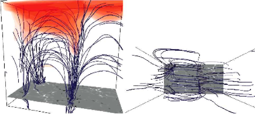
Figure 1: Computational box from the convection zone to the corona shown at time $500$ s as seen from the side (left panel) and from above (right panel). Lowest density is shown in red; compare that region with later stages (see figure 4). Magnetic field lines (blue) are mostly oriented along the $x$ axis. The vertical magnetic field in the photosphere is shown with a grey-scale layer.

Note that the atmosphere is very dynamic; the chromosphere, transition region and corona do not have borders at constant heights and the corrugated surfaces evolve in time; e.g., see figure 1 of Paper I. When discussing the results we therefore give the explicit heights of horizontal cuts and only sometimes an indication of the physical regime that dominates a given height range.

We have seeded the initial model with two different magnetic field configurations. In one sufficient stresses can be built up to maintain coronal temperatures in the upper part of the computational domain, as previously shown to be feasible by Gudiksen & Nordlund (2004). In the other models, the field is weaker and the corona slowly cools as the energy derived from foot point braiding is insufficient to maintain the initial coronal temperature. In these latter simulations (simulation A1 and A2) the average unsigned field strength in the photosphere is only $16$ Gauss and we find fairly weak coronal heating and temperatures of order $5\,10^{5}$ K and falling, while in the other (simulation B1) the average unsigned field strength is $155$ Gauss and the coronal temperature is of order $1$ MK or higher. The initial field in both cases was obtained by semi-randomly spreading some $20-30$ positive and negative patches of vertical field at the bottom boundary, and then calculating the potential field that arises from this distribution in the remainder of the domain. The field is advected by convective flows and photospheric motions and stresses sufficient to maintain a minimal corona which is built up by photospheric motions after roughly $20$ minutes solar time.

During this time we also find that the field topology is organized by the flow. After relaxation of the original field, the coronal loops in both sets of models are generally aligned along the $x$-axis, stretching from magnetic field concentrations centered roughly at $x=7$ Mm and $x=13$ Mm. The initial field geometry is shown in figure 1, where a subset of the field lines reaching the corona are shown from the side (in the left panel) and from above (right panel). Also shown in this figure is the distribution of the vertical magnetic field $B_{z}$ that pierces the photosphere (greyscale) and the regions of lowest mass density (in red), which in the initial model are concentrated near the top of the model, as expected. We shall later see that regions of low density can occur at lower heights after flux emergence has penetrated the corona.

3.1 Initial flux tube

We introduce a magnetic flux tube into the lower boundary of the model as described in detail in section 3.2 of Paper I. The magnetic flux tube structure is horizontally axisymmetric and the longitudinal field has a gaussian profile given by:

$${\bf B}_{l} = B_{o}\,\exp\left(-\frac{r^{2}}{R^{2}}\right)\,{\bf e}_{l},$$ (15)

$${\bf B}_{t} = B_{l}\,r\,q\,{\bf e}_{\phi},$$ (16)

where $r=\sqrt{(x-x_{o})^{2}+(z-z_{o})^{2}}$ is the radial distance to the center of the tube and $R$ is the radius of the tube. ${\bf B}_{l}$ and ${\bf B}_{t}$ are the longitudinal and transverse magnetic fields in cylindrical coordinates, respectively. The parameter $q$ is used by Linton et al. (1996) and Fan et al. (1998) to define the twist of the magnetic field. Following Cheung et al. (2006), we define a dimensionless twist parameter, $\lambda$, as:

$$\lambda\equiv q\,R.$$ (17)

As the flux tube enters the computational box, the height of the center of the tube ($z_{o}$) changes in time. The speed of the flux tube $({dz_{o}/dt})$ is set to the average of the velocity of the plasma inflow at the boundary in the region where the magnetic flux tube is located at each time step.

We have made three simulations (A1, A2, and B1): The emerging flux tube in runs A1 and A2 has the same strength, $B_{0}=4500$ Gauss at the bottom boundary, but the twist differs, $\lambda=0.3$ in simulation A1 and $\lambda=0.6$ in run A2. The latter simulation, B1, has a stronger pre-existing ambient field than the two others, while the injected field is weaker, $B_{0}=1100$ Gauss at the bottom boundary. The tube has no twist but a larger radius than simulations A1 and A2, and could indeed be described better as a flux slab than a flux tube. The emerging flux tubes injected at the bottom boundary are oriented in the $y$-direction and are centered roughly at 8 Mm in all three cases. A summary of the runs completed is shown in table 1. The magnetic energy of the tube is only a few times higher than the equipartition energy (defined as the average of the kinetic energy of the convective flows). The flux tube is weak enough to be perturbed and fragmented by the convective motions in all three models (in order to have a coherent tube the magnetic field energy would have to be more than 10 times more than the equipartion energy (e.g., Fan et al., 2003; Cheung et al., 2007). We don’t discuss that case here).

4 Results

In this paper we specifically concentrate on the later stages of the simulations where we study the evolution of the fields as it rises into the upper chromosphere and corona, the interaction between the field and the weak coronal magnetic field initially present, and the associated dynamics. In the following sections all the figures shown correspond to simulation A2 unless otherwise noted. This both because the A2 simulation has been run for the longest period of solar time ($>5000$ s) and, in addition, as it has the largest amount of magnetic flux emerging and passing into the outer layers.

The early stages of the flux emergence were covered in Paper I; for a summary see the introduction (section 1). Let us continue to follow the expansion of the field into the upper chromosphere and lower corona. As the magnetic flux moves into the upper chromosphere, it expands into the corona, pushing the coronal and transition region material aside, lifting and maintaining the transition region at heights greater than $5$ Mm above the photosphere for extensive periods of time. The cool magnetized bubbles reported in the chromosphere in Paper I gradually become elongated in the direction of the tube as they become weaker. They continue to thin until they disappear, and shock waves once again dominate the chromospheric dynamics. The pre-existing magnetic field in the corona and transition region is perturbed by the incoming flux and reoriented by a series of interactions between the two systems. A high density filamentary structure appears in the lower part of the flux tube and in regions below. While Joule heating is episodic, it increases in relative strength as fresh magnetic field rises and becomes energetically important in the upper chromosphere and corona at later times. All these processes will be described in the following sections.

4.1 The magnetic field

The only parts of the flux tube that can expand into the layers above the photosphere are those where the gradient of the magnetic field strength is larger than the superadiabatic excess in the photosphere. This relation between the buoyancy instability and the superadiabatic excess have been studied by several authors (Acheson, 1979; Magara & Longcope, 2001; Archontis et al., 2004). In Cheung et al. (2007) and in Paper I, it is pointed out that a greater amount of twist in the initial flux tube allows a larger fraction of magnetic flux to pass into the regions above the photosphere. The remaining parts of the magnetic field stay in the photosphere and move with the fluid into intergranular lanes where, eventually, the field is either pulled down into the convection zone or establishes enough of a gradient to be able to rise into the outer atmosphere. The expansion into the chromosphere does not happen uniformly, but rather in patches of several Mm² area. These regions of strong field remain in the same location in the chromosphere for several minutes and are related to the cold regions in the chromosphere described in Paper I.

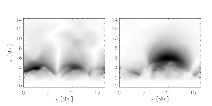
Figure 2: Vertical cut at $y=650$ km of the horizontal magnetic field strength normalized with the square root of the mean over the $y$ axis of the density. Two snapshots are shown: before the tube crosses the photosphere at time $600$ s (left-panel) and after the tube crosses the photosphere at $4200$ s (right panel). The panels are individually scaled: at time $4200$ s the maximum strength of the horizontal field is 3 times greater than at time $600$ s.

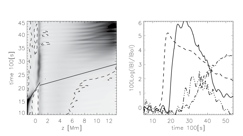
Figure 3: Ratio between the absolute horizontal and vertical magnetic field strength as averaged over the x and y axes as a function of time and height (left panel, see equation 18). The minimum value of the ratio is $7\,10^{-5}$ (white), while the maximum is $22.5$ (black). The regions where the ratio is greater than $1$ are delineated by the dashed lines. The average emergence velocity of the tube in the convection zone and the average expansion velocity of the tube above the photosphere are shown with straight solid lines. The right panel shows the average of the absolute magnetic field strength over specific height intervals and normalized with the same average taken over the first $500$ s of the simulation, see equation 21, in the upper convection zone ($z=[-854,-150]$ km, dashed line), the upper photosphere ($z=[106,490]$ km, solid line), the chromosphere ($z=[650,1130]$ km, dot-dot-dot-dashed line) and the corona ($z=[4108,12300]$ km, dot-dashed line).

The long term evolution of the coronal magnetic field is illustrated in figure 2 by showing the horizontal field at two times: before (left panel) and well after (right panel) the chromospherically buoyant regions of the tube have reached the corona (see also figure 3). In runs with no flux emergence the lower coronal field structure shown in the left panel of figure 2 has a lifetime of several hours, since the field that reaches to coronal heights is rooted well below the photosphere, where the timescales are correspondingly long. I.e. in the absence of flux emergence we would expect this general coronal field topology to be unvarying on timescales much longer than the simulations presented here. In the present case we do have flux emergence and the emerging flux tube’s axis reaches the photosphere at roughly 2000 s and remains in the vicinity of the photosphere/lower chromosphere until the end of the simulations (see also Fan, 2001; Magara & Longcope, 2003; Archontis et al., 2004; Manchester et al., 2004; Murray et al., 2006; Galsgaard et al., 2007). However, a portion of the tube expands upward and enough flux is transported to the upper-chromosphere to change the coronal field topology. This expansion happens at a fairly slow velocity, that decreases in time, but by $t=4200$ s figure 2 shows that the emerged flux completely dominates the upper chromosphere and lower corona.

Although it is almost impossible to follow the axis or the apex of the flux tube in these simulations because of the fragmented nature of the tube and its interaction with the ambient magnetic field. However, the rise of the tube and its subsequent expansion into the corona is nicely illustrated by following the evolution of the ratio between the horizontal and vertical magnetic field strength with height and time:

$$\frac{\langle|B_{h}|\rangle_{xy}}{\langle|B_{z}|\rangle_{xy}}$$ (18)

where $\langle\cdots\rangle_{xy}$ is the mean over $x$ and $y$ (see left panel of figure 3). We see that in the convection zone the flux tube rises at an average velocity of $3$ km s^-1. This velocity is similar to the mean upflow velocity of the convective motions but should also be compared with the buoyant velocity of the flux tube. The buoyant velocity is chosen as the terminal velocity between the buoyant force and the resistivity force:

$$u_{t}=\sqrt{\frac{\pi Rg}{C_{D}}\frac{\Delta\rho}{\rho}},$$ (19)

where $C_{D}$ is the drag coefficient and $\Delta\rho$ is the difference of the density inside the tube and its surroundings. We have chosen $C_{D}=2$ which seems suitable for our models. Assuming pressure equilibrium between the inside and outside of the tube we obtain

$$u_{t}\approx\sqrt{\frac{\pi Rg}{C_{D}}\frac{1}{\gamma\beta}}.$$ (20)

For simulations A1 and A2 this expression gives a buoyant velocity $u_{t}\approx 3$ km/s.

The expansion of the flux tube into the corona can also be followed in figure 3. The mean velocity of the expansion is roughly $16$ km s^-1, similar to the velocity of $17$ km s^-1 reported by Archontis et al. (2004). We also see an oscillatory wavelike pattern. Phases of large relative horizontal field seem to propagate into the corona like the rings that propagate when a stone is dropped into a pond. The horizontal field phase velocity is similar to the slow mode speed (around $30$ km s^-1 in the upper chromosphere) and at greater heights the phase speed can be seen to split to follow both slow mode and Alfvén speeds. The period of the oscillations is roughly $5$ minutes. Note that the field in the corona becomes steadily more horizontal as time progresses.

Looking in detail at the left panel of figure 3 we see that the ratio between horizontal and vertical field decreases as the flux tube gets closer to the photosphere ($z\approx 0$ km) from below. However, once the tube reaches the photosphere there is an increase of the relative horizontal field as the tube field “piles up”. Some $700$ s after the tube reaches the photosphere the ratio between horizontal and vertical field begins decreasing slowly due to flux expansion into the corona and some submergence of field back into the convection zone.

The right panel of figure 3 shows the evolution of flux emergence as function of height and time. To show the global behavior we take the average of the absolute magnetic field strength over specific height intervals and normalize with the same average taken over the first $500$ s of the simulation:

$$\frac{\langle|B|\rangle_{xy}(z,t)}{\langle|B|\rangle_{xyt[0:500]}(z)}$$ (21)

where $\langle\cdots\rangle_{xyt[0:500]}$ is the mean over $x$, $y$ and $t=[0:500]$ s. This procedure removes the pre-existing field and highlights the emerging flux. We show the evolution of this quantity as a function of time for four different height intervals: the upper convection zone (dashed line), the upper photosphere (solid line), the chromosphere (dot-dot-dot-dashed line) and the corona (dot-dashed line). Note the rapid increase and much more gradual decrease in the convection zone and photosphere and the more gradual emergence into the chromosphere and corona.

It is interesting to follow the evolution of the chromospheric and coronal field as the flux tube expands into the outer atmosphere. In figure 4 three sets of field lines are shown at $t=4500$ s. By this time the upper part of the expanding flux tube has risen into the corona and the associated field lines are drawn in blue. As these field lines rise, material drains along the field and a low density region is formed (shaded in red in figure 4). In response, the previously open field lines above the low density region (drawn in green) close and are pulled downwards. Not all of the expanding field makes it up into the corona; below the coronal portions of the rising flux we find field lines, (drawn in red) that remain in the chromosphere and are subject to the forced dynamics of that region. The highest (green) magnetic field lines are nearly horizontal near their apex, while the lower lying (blue) field lines have shapes that are much rounder.

Note that the three sets of field lines shown in figure 4 connect to different locations in the photosphere. The photospheric foot points of the coronal and chromospheric field lines are well concentrated but to different locations. By analyzing the velocity pattern at the bottom boundary, 1.4 Mm below the photosphere, we find that we can define a “mesogranular” scale that stretches over a scale equivalent to some $3-5$ granules horizontally. Field lines that are brought up by convection and/or in the rising flux tube first appear in the center of the granular cells. They are rapidly, in less than a minute, swept to the intergranular lanes. On a slower time scale, say roughly 30 minutes, the field lines are further transported to the boundaries of our “mesogranular” network (Stein & Nordlund, 2006). In our simulations different systems of field lines which have similar connectivity as they appear in the photosphere suffer reconnection amongst each other in the photosphere and lower chromosphere. After half an hour or so the flux is established in the “mesogranular” flow and the different systems are separated into discrete intermittent positions at the boundaries of mesogranular scale cells, see figure 4.

In the view seen from above (right panel, figure 4) the rotation of the originally x-oriented pre-existing ambient field in the corona is clear while comparing with figure 1. When the expanding portion of the flux tube reaches the corona, the direction of the field changes across the interface of the two flux systems (flux tube – pre-existing, ambient). The lower lying, deeper, lines (drawn in red) are more oriented in the same y direction as the emerging flux.

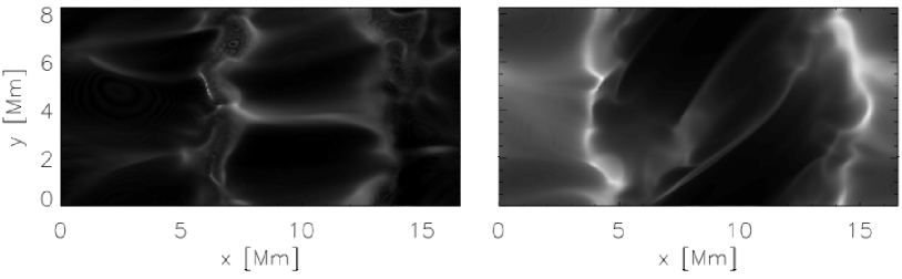
Figure 5: Disc center synthetic O vi image at times $700$ s (left panel) and $5280$ s (right panel).

The low density structure (shaded in red) is oriented in the $xy$ (diagonal) direction, evidence that the emerging flux and the ambient field have reconnected. This orientation is also evident in emission lines formed in the transition region and corona. An example of this is shown in figure 5 where the simulated intensity of the O vi $103.2$ nm emission line, formed at roughly $3\,10^{5}$ K, is displayed at two different times, before and after the flux expands into the corona. The O vi emission after flux emergence (right panel) clearly shows a large dark hole where the low density region is located. The high intensity regions of this line outlines the footpoints of hotter loops which are located deeper in the atmosphere where the densities are relatively large. In the A2 simulation we find that the low density region of the emerging flux found in the corona does not disappear; instead it increases in volume with time because the low density region expands horizontally while the downflow towards the loop foot points continues.

Late in the simulation, at time $4100$ s, small high density structures are pulled into the chromosphere with the expanding flux, these structures are associated with the chromospheric portion of the emerging flux tube (drawn in red) discussed above. Parts of these structures are visible in figure 4: below the large low density region (shaded red), high density (green-yellow) is visible at greater heights than in the surrounding atmosphere. After attaining a height of some $5$ Mm above the photosphere, the structures cease to rise, and while some of the plasma is trapped in magnetic dips and remains at great height, other plasma falls back towards the foot points (beginning roughly at $t=4400$ s). Dip like field configurations are produced naturally by the twist of the tube as noted by Aulanier & Demoulin (1998); López Ariste et al. (2006) and Magara (2007). The structures grow horizontally thinner as the flow drains to the foot points with a velocity around $20$ km s^-1 at $z\approx 4.1$ Mm. As they drain, the density contrast with the ambient chromosphere gradually fades and the structures are not discernible after $t=5000$ s.

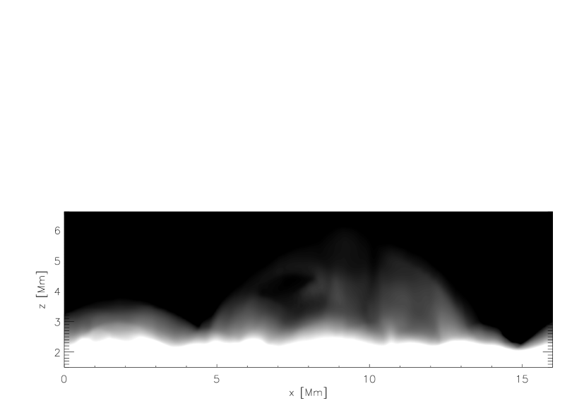
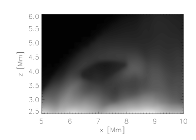
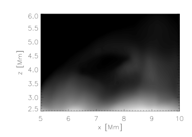
Figure 6: Ca ii H-line synthetic image at the limb at time $4640$ s (top panel) and a close-up showing the evolution of a dark feature at time $4610$ s (bottom left) and at time $4640$ s (bottom right).

Synthetic Ca ii H emission calculated at the limb (figure 6) show additional dynamics occurring in these high density structures. Evident is a dark structure which is moving upwards while expanding. The darkening is due to a small bubble, or low density inclusion, in the otherwise high density structure. The bubble is buoyant and moves upwards at roughly $10$ km/s. This low density bubble expands as mass drains from the upper layers of the high density structure surrounding it.

4.2 Joule-Heating

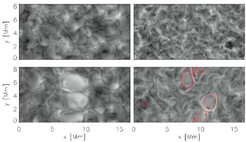
Figure 7: Joule heating in a logarithmic scale shown at $z=458$ km (left panels) and at $z=1100$ km (right panels) at times before the flux-tube reaches the photosphere at time $500$ s (top panels) and after the effects of the rising flux are evident at $2200$ s (bottom left panel) and $3390$ s (bottom right panel). Bright color corresponds to strong Joule heating. In order to show where the cold bubbles are, the bottom right panel includes a red contour where the temperature is 2300 K.

As the emerging flux expands into the chromosphere and corona the Joule heating rate increases. The increase of the heating rate with height closely follows the rise of flux as described in figure 2. While crossing the upper photosphere the spatial structure of this heating follows the magnetic field concentrations and is similar to the granular cell pattern as shown in figure 7 (left panel). The heating increases by more than a factor 3 in our simulations when the emerging flux crosses this height (458 km), but this is not enough to alter the temperature significantly. The increase in heating rate depends critically on the amount of magnetic flux that reaches the photosphere. In simulation A2 twice as much Joule heating occurs at this height as compared to simulation A1: the time scale for Joule heating $\tau=e/(\eta j^{2})$ is roughly $\tau=6000$ s for simulation A1 and $\tau=2500$ s for A2, during the time the major part of the Joule heating is due to the emerging flux. Thus, the greater the amount of magnetic flux that crosses the photosphere the greater the Joule heating.

The structure of the Joule heating is different in the chromosphere: the most important location of Joule heating is at the boundaries of the large cold magnetized bubbles that rise into the chromosphere and were described in Paper I. This is evident in the ellipsoidal structures that fit the boundaries of the cold bubbles (see the bottom right panel of figure 7). This heating pattern appears at the same time as the cold bubbles in the chromosphere, i.e. at $t=3100$ s, some $1250$ s after the tube has crossed the photosphere in model A2. The Joule heating associated with the flux expansion is more than a factor $10$ greater than that given by the pre-existing ambient field. It is also more energetically important at this height than in the upper photosphere: the time scale for Joule heating is $\tau=550$ s for simulation A1 and is $\tau=300$ s for A2.

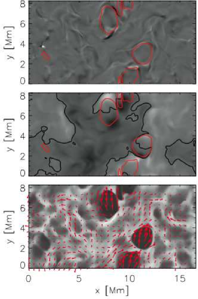
Figure 8: $z$-omponent of the vorticity (top panel), $z$-component of the magnetic field (middle panel) and the temperature (bottom panel) at $z=1100$ km and time $3390$ s. The red contours show where the temperature is 2300 K (top and middle panel) outlining the cold bubbles, the black contour is $B_{z}=0$ (middle panel) and the red vectors show the horizontal field direction (bottom panel).

The bubbles start to appear some $1100$ s after the tube crosses the photosphere and slowly move through the chromosphere during the next $1500-2000$ s. We find that the bubble shape becomes progressively rounder with greater magnetic field. Properties of the rising cold bubbles are shown in figure 8. The vertical field is positive in one half of the bubble and negative in the other half (middle panel). The horizontal magnetic field, on the other hand, is unidirectional across the bubble (lower panel) and the horizontal component of the field is larger than the vertical component. Inside the bubbles the mean ratio between the horizontal and vertical magnetic field, at $z=1100$ km, is 25.7 while the range is $[4081.8,0.23]$. As discussed above, we find that Joule heating is concentrated near the boundaries of the bubbles. This turns out to be true also for the vorticity, which is large in the vicinity of bubble boundaries (top panel). As time progresses the bubbles start to lose volume and become more elongated as the flux expands to greater heights and/or reconnects with the ambient field. After some 4800 s of run A2, the magnetically dominated cold bubbles are fully dispersed and the atmospheric state returns to a shock dominated chromosphere (e.g. Carlsson & Stein, 1992, 1995, 1997; Skartlien et al., 2000; Wedemeyer et al., 2004).

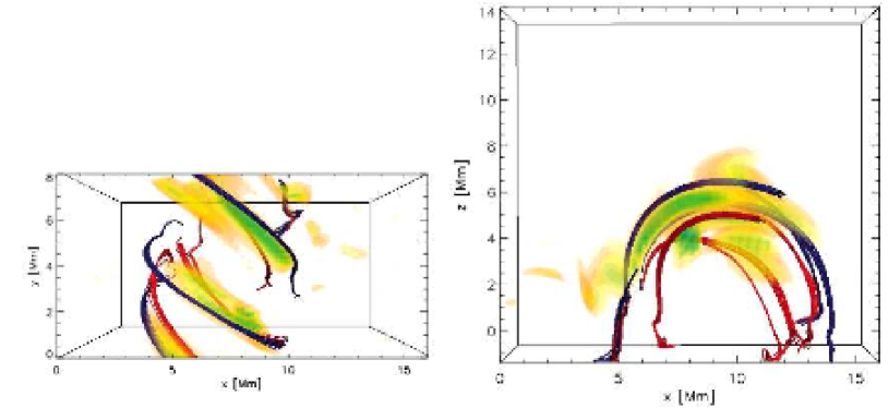
Figure 9: Computational box from the convection zone to the corona is shown at time $4200$ s from above (left panel) and from the side (right panel). Joule heating per particle is shown with yellow-blue color scale showing the banana structure. The magnetic field is shown above (blue) and below (red) two of these banana structures showing the discontinuity of the magnetic field.

As we move further up into the upper chromosphere and lower corona, magnetic field discontinuity and the associated Joule heating becomes progressively more important. In figure 9 we show the Joule heating at $t=4200$ s in the upper parts of the simulated atmosphere. The structure of Joule heating resembles bananas. In the upper chromosphere and lower corona the time scale of Joule heating is quite short ($\tau=10$ s at height 2.5 Mm and at time $4480$ s of simulation A2). At these heights, the Joule heating is of the same order as the thermal conduction and radiative losses. The field lines (shown in red) below the Joule heating structures are oriented along the emerging flux tube whereas the field lines above (shown in blue) are oriented more along with the pre-existing ambient field. Most of the banana shaped Joule heating structures in the simulations show this kind of discontinuity in the field line orientation.

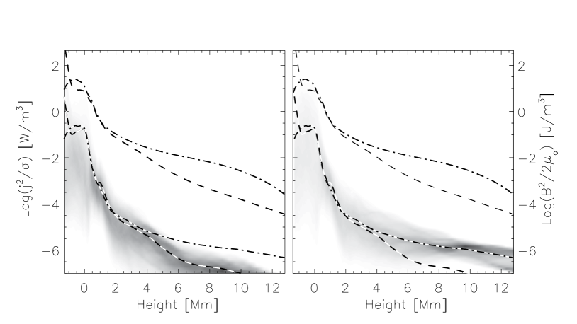
Figure 10: Distribution (pdf) of Joule heating as function of height at time $t=1400$ s (left panel) and at time $t=5460$ s (right panel) of the simulation A2. Also shown are the average of the Joule heating at time $1400$ s (lower dashed line) and at time $5460$ s (lower dash-dotted line) and the average magnetic field energy ${B^{2}/2\mu_{0}}$ as a function of height at time $1400$ s (upper dashed line) and at time $5460$ s (upper dash-dotted line).

It is not only the Joule heating rate in specific locations that increases with the introduction of emerging flux in the outer atmosphere, but also the general level of Joule heating throughout the upper chromosphere and corona. Figure 10 shows the probability distribution function of Joule heating through the entire atmosphere as a function of height at two instances; $t=1400$ s and $t=5460$ s, the former before the emerging flux enters the outer atmosphere, the latter after the flux has expanded into the corona. At the earlier time the total magnetic energy (${B^{2}/2\mu_{0}}$) varies from 0.5 J m^-3 in the mid chromosphere at $z=1$ Mm to $1.25\,10^{-4}$ J m^-3 high in the corona at $z=10$ Mm. Later, we find approximately the same average magnetic energy in the mid chromosphere, but it has increased greatly, a factor 20, in the corona to $2.5\,10^{-3}$ J m^-3 at $t=5460$ s. The Joule heating rate increases in a similar manner. At any given height the heating rate can vary horizontally by $1-3$ orders of magnitude, while the average heating rate decreases exponentially with height. At the earliest time, $1400$ s, when only the pre-existing field contributes, the average Joule heating is found to be $8\,10^{-4}$ W m^-3 at $z=1$ Mm, and less than $10^{-7}$ W m^-3 in the corona at $z=10$ Mm. At the later time we find the same heating rate at $1$ Mm, but the coronal heating rate at $10$ Mm has grown by an order of magnitude, to $8\,10^{-7}$ W m^-3.

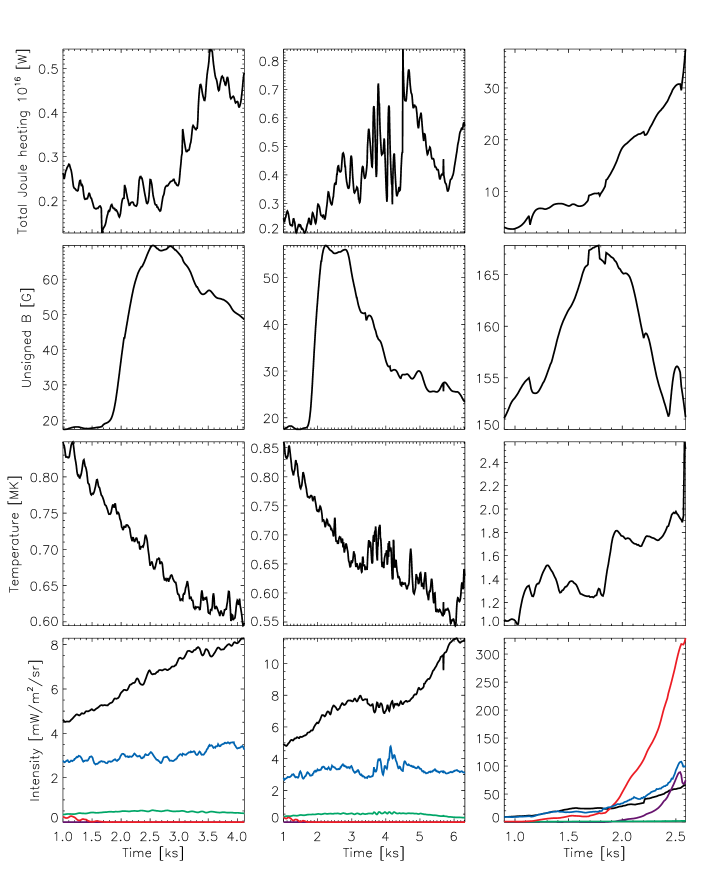
Figure 11: Integral of the Joule heating over the corona, i.e. the volume where the temperature is above $10^{5}$ K (top panels), unsigned magnetic field strength in the photosphere (second row of panels), maximum temperature (third row of panels) and mean emission of the He ii (blue line), O vi (black line), Ne viii (green line), Fe xii (red line) and Fe xv (violet line). Evolution shown for the simulation A1 (left column), A2 (middle column) and B1 (right column) as a function of time.

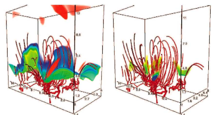
Figure 12: The computational box from the convection zone to the corona at time $4720$ s. The temperature in the transition region is shown with a yellow-blue color scale (left panel) with the highest temperatures shown in orange (up to $6\,10^{5}$ K). Joule heating is shown with a yellow-blue color scale (right panel). Both images include magnetic field lines shown in red.

In order to isolate coronal heating, we integrate the Joule heating over the entire volume constrained by the box edges where the plasma temperature is greater than $10^{5}$ K (see top row of figure 11). In simulation A2 (top middle panel), the total Joule heating increases from $t=2000$ s to $t=3700$ s as the flux emerges into the upper chromosphere and corona and interacts with the pre-existing ambient field. This heating increase is mostly confined to the extensions of the rising cool bubbles discussed earlier. From $t=3600$ s to $t=4200$ s the Joule heating in ‘banana-like’ structures appears, and the total Joule heating increases and shows greater variations with time. At $t=4700$ s there is a large jump in the total Joule heating in simulation A2. This large jump in the total Joule heating is related with the high temperatures close to the transition region ($>6\,10^{5}$ K shown in orange in the left panel of figure 12). Such blobs of hot plasma at the loop foot points near the transition region appear when the emerging flux comes in contact with the pre-existing ambient magnetic field, producing high Joule heating rate in a small region. The blob of hot plasma is first heated in the transition region but the high temperature rapidly (in some $20$ s) propagates into the corona by conduction. This process is repeated several times in the same vicinity roughly every 3 minutes. These oscillations are produced by the displacement of the transition region caused by the flux expansion which perturbs the atmosphere. This oscillatory movement stretches the flux tube lines with the ambient field lines, first in one specific region at one of the footpoint bands of the transition region and later at the opposite footpoint band. During these events the maximum temperature in the corona varies from $5.9\,10^{5}$ to $6.8\,10^{5}$ K. The first event is the strongest, after the strength of the Joule heating events decrease. The time scale of the Joule heating is in the first instance some $\tau=4.5$ s.

4.3 Coronal energy, temperature and Intensities

To further investigate the variation of the Joule heating in time and its possible effects on coronal energetics and diagnostics we return to figure 11 where we show the total Joule heating rate, along with the variation of the average photospheric magnetic field, the maximal coronal temperature, and some specific synthesized EUV resonance lines observable with spectrographs such as Hinode/EIS and SOHO/Sumer, as functions of time.

Let us first concentrate on simulation A1 (left column). The maximum temperature (third panel from the top) falls in time, indicating that the entire corona is cooling. The maximum temperature falls from some $8.5\,10^{5}$ K to $5.5\,10^{5}$ K from $t=1000$ s to $t=5700$ s. This is due to the imbalance between the heating and cooling processes; the Poynting flux being dissipated in the corona is not sufficient to balance thermal conduction and radiative losses. The paucity of coronal heating is primarily due to the weak pre-existing ambient field in the model. The average unsigned magnetic field strength in the photosphere is initially roughly $15$ G in runs A1 and A2. It stays almost constant until $t=1500$ s and then increases quickly up to $50$ G (A2) or $55$ G (A1); then stays constant for another 800 s. Afterwards, the field strength in the photosphere decreases to $25$ G for simulation A2 (at $5500$ s) and to $40$ G for simulation A1 (at $3500$ s). In the simulation B1 the field strength is initially $150$ G but increases to $162$ G (at $1500$ s), thereafter going down to $152$ G (at $2500$ s). We also find falling temperatures in the A2 simulation. However, note that in both simulations the drop in maximum temperature slows as the Joule heating increases at around $t=3500$ s. Note that the flux emerges into the corona already at $t=2000$ s, and needs some time to interact with the ambient field before any increase of the temperature is observed. In contrast to the runs A1 and A2 we find that in run B1 the maximum temperature does not decrease with time, but rather increases, from $1$ MK at $t=500$ s to nearly 2 MK at $t=2500$ s. This is presumably due to the much stronger pre-existing ambient field in this simulation (8 times larger than in the A1 and A2 simulations). In addition it is worth mentioning that the effects of flux emergence on the maximum coronal temperature occurs more rapidly in this run, almost immediately after the emerging flux enters into the corona.

In the bottom row of figure 11 we show the synthesized total intensity in various EUV spectral lines typical of different temperature regimes in the corona as a function of time. The synthesized intensity of these lines is computed assuming the optically thin approximation and may be written as

$$I={h\nu\over 4\pi}\int_{s}n_{\rm e}n_{\rm H}g(T_{\rm e})ds$$ (22)

where the integration is carried out along the line of sight, or in this case vertically through the box.

The He ii $25.6$ nm line is formed at some $8\,10^{4}$ K and is a typical lower transition region line, its total intensity is shown in blue in the bottom row of figure 11. We find that the intensity is roughly constant in the A1 and A2 simulations, though in the A1 run there is a slight increase in the intensity during the run and strong oscillations in the A2 run when the emerging flux perturbs the transition region. In the B1 run the He ii line intensity is initially of the same order, less than 10 mW m^-2sr^-1, but at the end of the run the intensity has risen quite substantially to almost 100 mW m^-2sr^-1. The O vi 103.2 nm line (drawn in black) formed at some $3\,10^{5}$ K rises from $5$ mW m^-2sr^-1 and essentially doubles during the A1 and A2 simulations. In the B1 run the O vi line rises from $5$ to $60$ mW m^-2sr^-1 during the time shown. The Ne viii $77$ nm line (drawn in green) is formed at $6.3\,10^{5}$ K, but remains weak, of order $1$ mW m^-2sr^-1, in all three simulations.

Finally, we show two coronal lines, Fe xii 19.5 nm formed at 1.25 MK and Fe xv 284 nm which is formed at 2 MK. These lines are negligible in the A1 and A2 runs but increase sharply with rising coronal temperatures in the warmer B2 simulation, where the radiative losses from Fe xii rise from $4$ to $20$ mW m^-2sr^-1 at $1600$ s, afterwards increase rapidly to greater than $300$ mW m^-2sr^-1 at $2300$ s, while the hot Fe xv line emits some $100$ mW m^-2sr^-1 at the end of the simulation.

Note that the Fe xv line follows the maximum temperature variation fairly accurately towards the end of the simulation with strong oscillations from $30$ to $90$ mW m^-2sr^-1 after $2200$ s. This is generally not the case, presumably because the total line intensity depends on both the density of the plasma emitting at the temperature of line formation and on the volume of emitting gas along the line of sight, which depends on the temperature gradient and/or topology of the corona. The relatively slow response of the coronal lines may reflect the significant timescales of heating or cooling significant amounts of material to or from coronal temperatures.

5 Discussion and Conclusions

Magnetic flux tube emergence is obviously important for the evolution of the magnetic field in the outer solar layers, but it is also of major significance in determining the dynamics and energetics of the chromospheric and coronal plasma.

We find that, after initially stalling in the photosphere, the emerging flux tube fragments, allowing discrete magnetized bubbles to expand into the chromosphere. It is almost impossible to follow the axis of the flux tube or its apex since the tube is shredded by plasma dynamics and mixes with the extant ambient magnetic field. This makes it difficult to study the velocity of the flux tube or its exact position. Nevertheless, what is clear is that the greater part of the flux tube is stuck in the upper photosphere; i.e. we do not observe any flux rope emergence in the regions above the photosphere. However, as mentioned, the upper parts of the magnetic flux tube expand into the corona. This expansion pushes the transition region upwards to at least $6$ Mm above the photosphere and also ensures that the regions of the upper chromosphere which contain the strongest field maintain a low density.

As the flux from the emerging tube crosses the chromosphere and corona, it interacts and eventually merges with the pre-existing ambient field. The resulting magnetic field configuration is a combination of the extant and newly emerging fields such that the direction of the resulting field lies between these two systems. The field from the emerging flux tube that rises into the corona also interacts with the pre-existing open field lines. These open field lines close and are seemingly pulled downward into the corona as at the same time the field lines from the expanding portion of the emerging field are moving upward. We find a low plasma density structure situated between these two systems of field lines. The low density structure is robust and lasts for more than thirty minutes. It is produced by a downflow from the lower corona to the photosphere following the field lines. The total pressure in the low density region is lower than the total pressure in the field line systems above and below resulting in them getting closer to each other. The pressure imbalance is partly offset by magnetic tension forces which slows the process.

Just below the low density structure we find that a high density structure forms in the chromosphere. This structure rises with the expanding field lines and is maintained at above hydrostatic heights by a dip-like structure of the magnetic field that is produced naturally by the twist in the expanding field. The structure thins with time as portions of its mass drain to the foot points of the supporting magnetic field lines. The structure described is in some ways suggestive of solar quiescent filaments even though filaments are much larger scale structures that are, as yet, impossible to simulate with the type of simulation described here.

Associated with the high density structure we also find low density inclusions that display interesting dynamics shown in the synthetic Ca ii images at the limb that resembles dynamics observed in quiescent prominences with the Hinode spacecraft (Berger et al., 2008). The low density structure moves upwards at buoyant velocity and expands as material drains out of the regions above it. Even so, we are hard pressed from finding counterparts to all of the dynamic phenomena observed at the solar chromospheric limb with Hinode or the Swedish 1-meter Solar Telescope.

The emerging field lines that remain in the lower chromosphere become more tangled than those that expand all the way into the corona where the field has more or less uniform direction. The foot points of the various field lines systems are connected intermittently in the network situated in the boundaries of the “mesogranular” scales discussed in Section 4.1. The field from different heights seems to concentrate in different intermittent “mesogranular” regions which all evolve on timescales typical of the convective layers below the photosphere.

One of our goals is to study the Joule heating produced by interaction between the emerging flux and the pre-existing ambient magnetic field. In these simulations we have run two cases with weak pre-existing magnetic field and fairly strong emerging field and one case with a stronger pre-existing field and a weak emerging field. In all cases the Joule heating increases throughout the atmosphere as the emerging field expands, but it seems that the additional Joule heating is more vigorous when the pre-existing field is stronger.

The Joule heating caused by emerging flux is localized and surrounds the cool magnetized bubbles that rise into the chromosphere, and at later times form elongated structures. Joule heating is energetically more important in the chromosphere than in the photosphere and increases in importance at even greater heights to become a dominant term in the energetics in the corona. The structure of the Joule heating in the upper-chromosphere and corona takes on banana shaped forms that follow the magnetic field lines.

Joule heating has both a quasi-stationary component as well as occurring in episodic events of larger amplitude. The latter is evident in the corona as high temperature blobs are produced, as a rule near the transition region interface. Thus, near the foot points of a coronal loop, high temperature gas is formed in discrete bursts. The injected heat moves into the higher layers of the corona as a result of thermal conduction, on short timescales. Such energetic episodic events are often repeated several times, in the same place, but they becomes weaker with each repetition.

Flux emergence changes the total emission of various transition region and coronal lines. In general the emission of O vi and Ne viii increases as emerging flux expands into the corona. However, in the runs with a weak pre-existing magnetic field the temperature remains too low to give rise to emission in coronal lines such as Fe xii or Fe xv. In the strong field case these lines increase their intensity very rapidly, at the end of the run the Fe xii is the strongest line of those modeled. In no case do we find a one-to-one correspondence between the variations of the temperatures and the line intensity of the coronal lines. When the corona is heated more matter is brought to coronal temperatures. In addition, the density rises which occurs on a different, generally longer, timescale than the heating timescale which governs the evolution of the temperature. The resulting line emission reflects a combination of these time scales.

6 Acknowledgments

This research has been supported by a Marie Curie Early Stage Research Training Fellowship of the European Community’s Sixth Framework Programme under contract number MEST-CT-2005-020395: The USO-SP International School for Solar Physics. Financial support by the European Commission through the SOLAIRE Network (MTRN-CT-2006-035484) and by the Spanish Ministry of Research and Innovation through project AYA2007-66502 is gratefully acknowledged. This research was supported by the Research Council of Norway through grant 170935/V30 and through grants of computing time from the Programme for Supercomputing. To analyze the data we have used IDL and Vapor (http://www.vapor.ucar.edu). Sven Wedemeyer-Böhm, Jorrit Leenaarts and Chung Ming Mark Cheung are thanked for valuable discussions and comments.

Figure 4: Computational box from the convection zone to the corona at time $4500$ s as seen from the side (left panel) and from above (right panel). Density is shown in color: blue-green-yellow-red in order of decreasing density (compare with figure 1). Magnetic field lines are drawn from regions of low density (blue lines), high density regions (red lines) and where the magnetic field was open $400$ s before (green). The temperature in the photosphere is shown with a grey-scale layer.

Table 1: Summary of parameters for the three simulations

Name	Twist $\lambda$	B0 [G]	Size [$Mm^{3}$]	Time [s]	Radius [Mm]	Ambient field [G]
A1	0.3	4484	$16\times 8\times 16$	4200	0.5	16
A2	0.6	4484	$16\times 8\times 16$	6300	0.5	16
B1	0	1121	$16\times 8\times 16$	2600	1.5	155

References

- Abbett (2007) Abbett W. P., 2007, ApJ, 665, 1469
- Acheson (1979) Acheson D. J., 1979, Sol. Phys., 62, 23
- Archontis et al. (2004) Archontis A., Moreno-Insertis F., Galsgaard K., Hood A., O’Shea E., 2004, A&A, 426, 1047
- Aulanier & Demoulin (1998) Aulanier G., Demoulin P., 1998, A&A, 329, 1125
- Berger et al. (2004) Berger T. E., Rouppe van der Voort L. H. M., Löfdahl M. G., et al., 2004, A&A, 428, 613
- Berger et al. (2008) Berger T. E., Shine R. A., Slater G. L., et al., 2008, ApJ, 676, L89
- Carlsson & Stein (1992) Carlsson M., Stein R. F., 1992, ApJ, 397, L59
- Carlsson & Stein (1995) Carlsson M., Stein R. F., 1995, ApJ, 440, L29
- Carlsson & Stein (1997) Carlsson M., Stein R. F., 1997, ApJ, 481, 500
- Cheung et al. (2006) Cheung M. C. M., Moreno-Insertis F., Schüssler M., 2006, A&A, 451, 303
- Cheung et al. (2007) Cheung M. C. M., Schüssler M., Moreno-Insertis F., 2007, A&A, 467, 703
- Fan (2001) Fan Y., 2001, ApJ, 554, L111
- Fan et al. (2003) Fan Y., Abbett W. P., Fisher G. H., 2003, ApJ, 582, 1206
- Fan et al. (1998) Fan Y., Zweibel E. G., Linton M. G., Fischer G. H., 1998, ApJ, 505, L59
- Galsgaard et al. (2007) Galsgaard K., Archontis V., Moreno-Insertis F., Hood A. W., 2007, ApJ, 666, 516
- Gudiksen & Nordlund (2004) Gudiksen B. V., Nordlund Å., 2004, en IAU Symposium, Vol. 219, Dupree A. K., Benz A. O. (eds.), Stars as Suns : Activity, Evolution and Planets, p. 488
- Gudiksen & Nordlund (2005) Gudiksen B. V., Nordlund Å., 2005, ApJ, 618, 1020
- Hansteen et al. (2007) Hansteen V. H., de Pontieu B., Carlsson M., et al., 2007, PASJ, 59, 699
- Jouve & Brun (2007) Jouve L., Brun A. S., 2007, Astronomische Nachrichten, 328, 1104
- Kosovichev & Duvall (2008) Kosovichev A. G., Duvall T. L., Jr., 2008, Local Helioseismology and Magnetic Flux Emergence, en Astronomical Society of the Pacific Conference Series, Vol. 383, Howe R., Komm R. W., Balasubramaniam K. S., Petrie G. J. D. (eds.), p. 59
- Linton et al. (1996) Linton M. G., Longcope D. W., Fisher G. H., 1996, ApJ, 469, 954
- López Ariste et al. (2006) López Ariste A., Aulanier G., Schmieder B., Sainz Dalda A., 2006, A&A, 456, 725
- Magara (2007) Magara T., 2007, PASJ, 59, L51
- Magara & Longcope (2001) Magara T., Longcope D. W., 2001, ApJ, 559, L55
- Magara & Longcope (2003) Magara T., Longcope D. W., 2003, ApJ, 586, 630
- Manchester et al. (2004) Manchester W., IV, Gombosi T., DeZeeuw D., Fan Y., 2004, ApJ, 610, 588
- Martínez-Sykora et al. (2008) Martínez-Sykora J., Hansteen V., Carlsson M., 2008, ApJ, 679, 871
- Moreno-Insertis & Emonet (1996) Moreno-Insertis F., Emonet T., 1996, ApJ, 472, L53
- Murray et al. (2006) Murray M. J., Hood A. W., Moreno-Insertis F., Galsgaard K., Archontis V., 2006, A&A, 460, 909
- Rouppe van der Voort et al. (2005) Rouppe van der Voort L. H. M., Hansteen V. H., Carlsson M., et al., 2005, A&A, 435, 327
- Skartlien et al. (2000) Skartlien R., Stein R. F., Nordlund Å., 2000, ApJ, 541, 468
- Stein & Nordlund (2006) Stein R. F., Nordlund Å., 2006, ApJ, 642, 1246
- Wedemeyer et al. (2004) Wedemeyer S., Freytag B., Steffen M., Ludwig H.-G., Holweger H., 2004, A&A, 414, 1121