Hadronisation Corrections for Jets in the $k_{t}$ Algorithm

Abstract

It has recently been established that hadronisation corrections to QCD jets vary as $1/R$, at small $R$, for jets of radius $R$. Here we demonstrate, using jets in the $k_{t}$ algorithm, that the magnitude of these $1/R$ corrections are unambiguously linked to the magnitude of $1/Q$ corrections to commonly studied event shapes in $e^{+}e^{-}$ annihilation.

MAN/HEP/2009/30

1 Introduction

An understanding of QCD jets and their properties will be integral to the success of the LHC physics program. In particular one of the most important issues in current jet studies is the question of jet energy scale. The shift induced in jet energy by effects such as perturbative radiation and non-perturbative effects like hadronisation and the underlying event would contribute to a smearing of, for instance, mass peaks that may be a signal for new physics. Thus in order to choose optimal jet definitions that minimise such smearing one would need to know the dependence of the above effects on the experimental parameters like jet radius. Moreover, even in pure QCD studies such as the extraction of parton distribution functions (pdfs) and the strong coupling $\alpha_{s}$ from jet observables like the inclusive jet cross-sections, a knowledge of the non-perturbative contribution is important to supplement perturbative calculations. A relatively small shift in the transverse momentum $p_{t}$ of a jet, induced by hadronisation, can result in a significant change in the inclusive jet spectrum since we are dealing with a quantity that has a steeply falling $p_{t}$ distribution.

While it is traditional to study the hadronisation contribution via Monte Carlo models such as those in HERWIG and PYTHIA, it turns out that in cases like the jet energy there is additionally valuable analytical insight available [2]. Analytical models based on renormalons [3] have in the past been met with great success in the description of LEP and HERA event-shape variables [4], but have not really been utilised outside that context. In Ref. [2] one such model (due to Dokshitzer and Webber [5]) was used to estimate hadronisation corrections to jet transverse momentum $p_{t}$. The result found there was striking: hadronisation effects have a singular $1/R$ dependence on the jet radius $R$, at small $R$. This is in complete contrast to the contribution from the underlying event which varies as $R^{2}$. The knowledge of the $R$ dependence of non-perturbative effects in conjunction with the $\ln R$ behaviour involved in perturbative estimates can then be used to arrive at conclusions about the optimal values of $R$ to be used in diverse studies involving jets, as exemplified in Ref. [2].

While the computations of Ref. [2] indicate the dependence of hadronisation corrections and the underlying event on $R$, there remains the question of the overall magnitude of these effects. While for the underlying event one is reliant solely on Monte Carlo event generators to obtain the overall magnitude, for the hadronisation correction a tentative link was made in Ref. [2] between the magnitude of the $1/R$ correction and that of $1/Q$ corrections to LEP and HERA event shapes such as the thrust distribution (see [4] for a review). In order to definitely link the magnitude of jet hadronisation to that of event-shape power corrections one needs to carry out a calculation at the two-loop level rather than the simple one-loop estimate reported in [2]. The calculation for jets defined in the $k_{t}$ algorithm [6, 7] is reported here while the corresponding result for jets in the anti-$k_{t}$ algorithm is already known [8]. Work on the other jet algorithms is currently in progress.

2 The single-gluon result

In the Dokshitzer-Webber model non-perturbative hadronisation corrections are associated to the emission of a soft gluon with transverse momentum $k_{t}\sim\Lambda_{\mathrm{QCD}}$. For the jet $p_{t}$ case we work out the change in transverse momentum $\delta p_{t}$ induced by the emission of such a gluon and combined with the gluon emission probability (as given by perturbative QCD) this yields the average shift in $p_{t}$ induced by hadronisation:

$$\langle\delta p_{t}\rangle^{h}\sim\frac{C_{j}}{2\pi}\int\frac{dk_{t}}{k_{t}}d\eta\frac{d\phi}{2\pi}\,\delta p_{t}(k)\,\alpha_{s}(k_{t}),$$ (1)

where $k_{t}$, $\eta$ and $\phi$ respectively denote the transverse momentum, rapidity and azimuth of the emitted gluon with respect to the emitting hard parton (jet) and $C_{j}$ is the colour factor associated to emission from the given hard parton. The reason we are able to single out a given hard parton initiating a high-$p_{t}$ jet in any hard process is essentially since the leading $1/R$ result stems from emission collinear to the triggered jet. It is thus possible to talk in terms of the single-jet limit ignoring the rest of the details of the hard process.

The only non-perturbative ingredient that is involved above is the value of $\alpha_{s}(k_{t})$ at scales around or below $\Lambda_{\mathrm{QCD}}$. If one makes the assumption of a universal infrared-finite coupling, which replaces the perturbative coupling that has an unphysical divergence at $\Lambda_{\mathrm{QCD}}$, then one arrives at a prediction for the hadronisation correction $\langle\delta p_{t}\rangle^{h}$. Using the fact [2] that the $\delta p_{t}(k)$ is essentially the energy of the gluon emitted outside the jet we perform the integral over rapidity in Eq. (1) to obtain the leading $1/R$ behaviour. The result is of the form $c\,{\mathcal{A}}/R$, where $c$ is a number obtained from the rapidity integral and ${\mathcal{A}}$ is the moment of the coupling $\alpha_{s}(k_{t})$ over the infrared region (we refer the reader to Refs. [9, 10] for the precise details). Since the same coupling moment enters the predictions for event-shape variables we can take its value from data on event shapes and hence obtain a numerical prediction for the leading $1/R$ hadronisation correction to jet $p_{t}$. This was the method adopted in Ref. [2].

Here we point out a limitation of the above approach [11] which is that while we have written down and used a running coupling $\alpha_{s}(k_{t})$, this quantity only emerges when one considers not just the emission of a single gluon but in fact gluon decay as well. To be precise an inclusive integration over gluon decay products is responsible for building up the quantity $\alpha_{s}(k_{t})$. Unfortunately, as is known for event-shape variables, our observable is sensitive to the precise details of gluon branching and hence one is not free to carry out such an inclusive integration. One must therefore return to the details of the gluon branching and identify the correction to the above inclusive approximation. The analysis at this level has already been carried out for event-shape variables [9, 10, 12, 13] and below we report on it for the jet $p_{t}$ case.

3 Non-perturbative effects and gluon decay

Now we consider the situation where the emitted gluon with $k_{t}\sim\Lambda_{\mathrm{QCD}}$ is allowed to decay and at the same accuracy account for virtual corrections to single gluon emission, as depicted in Fig. 1.

At this two-loop level the change in $p_{t}$ (for a quark jet) can be expressed as:

$$\langle\delta p_{t}\rangle^{h}=\frac{C_{F}}{\pi}\int\frac{d^{2}k_{t}}{\pi k_{t}^{2}}\frac{d\alpha}{\alpha}\left\{\alpha_{s}(0)+4\pi\chi(k_{t}^{2})\right\}\delta p_{t}(k)+4C_{F}\int\left(\frac{\alpha_{s}}{4\pi}\right)^{2}d\Gamma_{2}\frac{M^{2}}{2!}\delta p_{t}(k_{1},k_{2}),$$

Figure 1: Gluon decay and one-loop corrections to single-gluon emission.

where $\alpha$ is a Sudakov variable, $\alpha_{s}(0)$ is an ill-defined quantity which will cancel away subsequently, $\chi$ represents the virtual correction to gluon emission, $d\Gamma_{2}$ is the gluon decay phase-space and $M^{2}$ is the decay matrix element [9, 10]. We also denote by $\delta p_{t}(k_{1},k_{2})$ the change in $p_{t}$ due to correlated two-parton emission while $\delta p_{t}(k)$ is the corresponding single-gluon quantity. To correctly account for gluon branching one thus has to perform the above calculation, the details of which are reported in Ref. [14].

The analogous two-loop analysis for event-shape variables [9, 10, 12, 13] revealed an initially surprising result – the two-loop correction simply provided a universal rescaling factor to the one-gluon result, which became known as the Milan factor. Its value for $n_{f}=3$ (which is the number of flavours excited in the relevant soft region) was found to be $\mathcal{M}=1.49$. Thus the ratio of corrections to two event shapes $v_{1}$ and $v_{2}$ was merely the ratio of the one-loop coefficients computed previously [5]:

$$\frac{\delta v_{2}^{\mathrm{NP}}}{\delta v_{1}^{\mathrm{NP}}}=\frac{\delta v_{2}^{\mathrm{NP},1}}{\delta v_{1}^{\mathrm{NP},1}},$$

where $\delta v_{1}^{\mathrm{NP},1}$ denotes the non-perturbative single-gluon correction for $v_{1}$ computed as discussed in the preceding section and likewise for $v_{2}$. This remarkable result was understood to arise as a consequence of the fact that all the variables considered could be expressed as linear sums over the transverse momenta $k_{ti}$ of emissions, $v=\sum_{i}k_{ti}c_{i}$, where the $c_{i}$ are rapidity-dependent coefficients [10].

In the case of jet $p_{t}$ this linear dependence is ruined by the non-trivial action of the jet algorithm in all cases except the case of jets defined in the anti-$k_{t}$ algorithm [8]. The contribution to the jet $\delta p_{t}$ of a given emission is found to be of the form $k_{t}e^{\eta}\,\Xi_{\mathrm{out}}$, where $\eta$ denotes the rapidity with respect to the emitting hard jet and $\Xi_{\mathrm{out}}$ denotes the condition that the emission ends up outside the jet after the application of the jet algorithm. It should be immediately clear from this that in most current sensible jet algorithms (both of sequential recombination and cone type) the condition $\Xi_{\mathrm{out}}$ is non-trivial and introduces non-linearity in $k_{t}$. For instance in the $k_{t}$ algorithm we can consider the situation in Fig. 2, where although one may have a soft parton separated by more than a certain distance $R$ in rapidity and azimuth (denoted by the red gluon line) from a given hard parton, it may be clustered to another soft parton (denoted by the black gluon line) and hence swept into the final jet. This clustering depends on the $k_{t}$ of a soft parton relative to the other partons and hence the condition $\Xi_{\mathrm{out}}$ derived in [14] contains dependence on the $k_{t}$ of the soft partons, spoiling the simple linear dependence needed for universality.

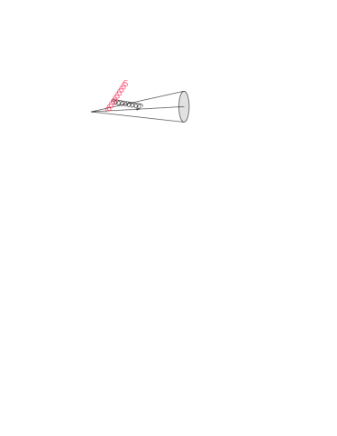
Figure 2: The role of clustering in determining whether a soft gluon ends up within or outside a hard jet.

An exception to the above situation is to be found in the anti-$k_{t}$ algorithm for which the condition $\Xi_{\mathrm{out}}=\Theta(\eta^{2}+\phi^{2}-R^{2})$ ensures that a given parton is outside the jet if its angular ($\eta,\phi$) separation from the hard jet is more than $R$. The linear dependence on $k_{t}$ is maintained and the Milan factor $\mathcal{M}=1.49$ is computed as for event shapes.

For the $k_{t}$ algorithm we have carried out an equivalent calculation for the leading $1/R$ hadronisation correction (at small $R$) with the more complicated $\Xi_{\mathrm{out}}$ function involved there and we found the result $\mathcal{M}_{k_{t}}=1.01\,(n_{f}=3)$. Thus while at the level of the one-gluon studies of Ref. [2] the $k_{t}$ and anti-$k_{t}$ algorithms received identical hadronisation corrections, a detailed analysis at the two-loop level breaks this equality. One finds that the ratio of hadronisation corrections is then:

$$\frac{{\langle\delta p_{t}\rangle}^{h}_{k_{t}}}{{\langle\delta p_{t}\rangle}^{h}_{\mathrm{anti-}k_{t}}}=\frac{1.01}{1.49}\sim 0.7\,.$$

Thus one expects somewhat smaller hadronisation corrections for the $k_{t}$ algorithm as compared to those for the anti-$k_{t}$ algorithm which is also borne out by the Monte Carlo studies with HERWIG and PYTHIA reported in Ref. [2]. We remind the reader that these conclusions apply only to the $1/R$ hadronisation corrections that would be dominant at small $R$ and we neglect finite $R$ corrections which need to be considered alongside the underlying event contribution which also has a regular $R$ dependence $\sim R^{2}$.

4 Conclusions

We have reported on a study of hadronisation corrections to jet $p_{t}$ or energy scale based on two-loop extensions of the one-gluon estimates reported in Ref. [2], with jets defined in the $k_{t}$ algorithm. Studies for other jet algorithms (SISCone [15] and Cambridge/Aachen [16]) are in progress.

References

-
[1]
Slides:
http://indico.cern.ch/contributionDisplay.py?contribId=250&sessionId=3&confId=53294 - [2] M. Dasgupta, L. Magnea and G. P. Salam, JHEP 02 (2008) 055 [arXiv:0712.3014 [hep-ph]].
- [3] M. Beneke, Phys. Rept. 317 (1999) 1 [arXiv:hep-ph/9807443].
- [4] M. Dasgupta and G. P. Salam, J. Phys. G 30 (2004) R143 [arXiv:hep-ph/0312283].
- [5] Y. L. Dokshitzer and B. R. Webber, Phys. Lett. B 352 (1995) 451 [arXiv:hep-ph/9504219].
- [6] S. D. Ellis and D. E. Soper, Phys. Rev. D 48 (1993) 3160 [arXiv:hep-ph/9305266].
- [7] S. Catani, Y. L. Dokshitzer, M. H. Seymour and B. R. Webber, Nucl. Phys. B 406 (1993) 187.
- [8] M. Cacciari, G. P. Salam and G. Soyez, JHEP 04 (2008) 063 [arXiv:0802.1189 [hep-ph]].
- [9] Y. L. Dokshitzer, A. Lucenti, G. Marchesini and G. P. Salam, Nucl. Phys. B 511 (1998) 396 [Erratum-ibid. B 593 (2001) 729] [arXiv:hep-ph/9707532].
- [10] Y. L. Dokshitzer, A. Lucenti, G. Marchesini and G. P. Salam, JHEP 05 (1998) 003 [arXiv:hep-ph/9802381].
- [11] P. Nason and M. H. Seymour, Nucl. Phys. B 454 (1995) 291 [arXiv:hep-ph/9506317].
- [12] M. Dasgupta, L. Magnea and G. Smye, JHEP 11 (1999) 025 [arXiv:hep-ph/9911316].
- [13] M. Dasgupta and B. R. Webber, JHEP 10 (1998) 001 [arXiv:hep-ph/9809247].
- [14] M. Dasgupta and Y. Delenda, arXiv:0903.2187 [hep-ph].
- [15] G. P. Salam and G. Soyez, JHEP 05 (2007) 086 [arXiv:0704.0292 [hep-ph]].
-
[16]
Y. L. Dokshitzer, G. D. Leder, S. Moretti and B. R. Webber,
JHEP 08 (1997) 001 [arXiv:hep-ph/9707323];
M. Wobisch and T. Wengler, arXiv:hep-ph/9907280.