Spectrum of Fractal Interpolation Functions

Abstract

In this paper we compute the Fourier spectrum of the Fractal Interpolation Functions FIFs as introduced by Michael Barnsley. We show that there is an analytical way to compute them. In this paper we attempt to solve the inverse problem of FIF by using the spectrum

1 Iterated Function Systems

The affine transform performs translation stretching and rotation on a given set. In the special case of two dimensions the affine transform on a set $\mathcal{S}$ in 2-D space is described by the equation:

$$w(x,y)=\left[\begin{array}[]{cc}a&b\\ c&d\\ \end{array}\right]\left[\begin{array}[]{c}x\\ y\\ \end{array}\right]+\left[\begin{array}[]{c}e\\ f\\ \end{array}\right]$$

where $(x,y)\in{\mathcal{S}}$. The effects of an affine transform on a set are depicted in fig. 1. The union of N affine transformations is called the Hutchinson operator: $W=\bigcup_{n=1}^{N}w_{n}$. For a specified metric the distance $h({\mathcal{A},B})$ between two sets ${\mathcal{A},B}$ can be defined. Under certain conditions [2] the Hutchinson operator is contractive, $h(W({\mathcal{A}}),W({\mathcal{B}}))\leq sh({\mathcal{A},B}),\quad s<1$. Successive iterations with Hutchinson operator on a random set results in a sequence of a sets that converges in the attractor of the operator $\mathcal{A}$, which satisfies the condition ${\mathcal{A}}=W({\mathcal{A}})=\bigcup_{n=1}^{N}w_{n}({\mathcal{A}})$. Any system that uses the Hutchinson operator in order to generate iteratively the attractor $\mathcal{A}$ is called Iterated Function System (IFS).

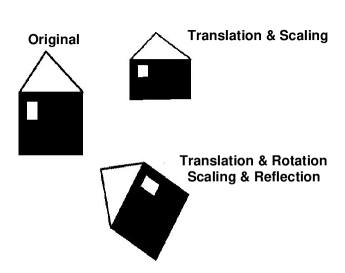
Figure 1: An affine transform can translate rotate and flip a 2-dimensional shape.

1.1 Fractal Interpolation Functions

Fractal Interpolation Functions (FIF) is a special case of the 2-dimensional IFS and maintain all their characteristics. FIF attractors are continuous functions that can be used to model continuous signals. FIF interpolate a given set of $N+1$ points $(x_{n},y_{n}),\quad n=0,1\dots N$

$$x_{0}<x_{1}<x_{2}<x_{3}<\dots<x_{N}$$

The FIF that interpolates the above set is comprised of $N$ affine maps:

$$w_{n}\left[\begin{array}[]{c}x\\ y\end{array}\right]=\left[\begin{array}[]{cc}a_{n}&0\\ c_{n}&d_{n}\end{array}\right]\left[\begin{array}[]{c}x\\ y\end{array}\right]+\left[\begin{array}[]{c}e_{n}\\ f_{n}\end{array}\right],n=1,\dots,N.$$

The necessary condition is that the Interpolation Function passes from the $N+1$ initial points,

$$w_{n}\left[\begin{array}[]{c}x_{0}\\ y_{0}\end{array}\right]=\left[\begin{array}[]{c}x_{n-1}\\ y_{n-1}\end{array}\right]\mbox{ and }w_{n}\left[\begin{array}[]{c}x_{N}\\ y_{N}\end{array}\right]=\left[\begin{array}[]{c}x_{n}\\ y_{n}\end{array}\right]\quad,$$ (1)

$$n=1,\dots,N$$

We call order of the FIF, the number $N$ of the affine maps. The conditions provide 4 equations for 5 parameters , so $d_{n}$, the vertical scaling factor is chosen to be the free parameter. If we solve the above equations for $a_{n},c_{n},e_{n},f_{n}$ in terms of $d_{n}$, we find :

$$a_{n} = \frac{x_{n}-x_{n-1}}{x_{N}-x_{0}},$$ (2)

$$e_{n} = \frac{x_{N}x_{n-1}-x_{0}x_{n}}{x_{N}-x_{0}},$$ (3)

$$c_{n} = \frac{y_{n}-y_{n-1}}{x_{N}-x_{0}}-\frac{d_{n}(y_{N}-y_{0})}{x_{N}-x_{0}},$$ (4)

$$f_{n} = \frac{x_{N}y_{n-1}-x_{0}y_{n}}{x_{N}-x_{0}}-d_{n}\frac{x_{N}y_{0}-x_{0}y_{N}}{x_{N}-x_{0}}.$$ (5)

Let the real numbers $a_{n},c_{n},e_{n},f_{n}$ be defined by (2-5). Barnsley [2] introduced the operator $T$ for the class $\mathcal{C}$ of continuous functions, $T:\mathcal{C}\rightarrow\mathcal{C}$ by

$$(TF)(x)=c_{n}\ell_{n}^{-1}(x)+d_{n}F(\ell_{n}^{-1}(x))+f_{n}\quad$$

$$\forall x\in[x_{n-1},x_{n}]\;\;,n=1,2\dots,N,$$

and

$$\ell_{n}:[x_{0},x_{N}]\rightarrow[x_{n-1},x_{n}]$$

the invertible transformation

$$\ell_{n}(x)=a_{n}x+e_{n}.$$

The above operator:

• is a contraction mapping according to Hausdorff metrics,

• satisfies the conditions of (1),

• has a unique fixed point, the function $F\in\mathcal{C},$

  $$(TF)(x)=F(x),\quad\forall x\in[x_{0},x_{N}].$$

The following restrictions guarantee the contractivity of $T$ operator:

• $\;a_{n}\;<1$

• $|d_{n}|<1.$

Barnsley’s operator is very useful because the attractor of an FIF can be generated with the iterative application of $T$ on an initial signal $F(0)$ : $F_{m+1}=TF_{m}$,

$$F=\lim_{m\rightarrow\infty}T^{\circ m}(F_{0}),F_{0}\in\mathcal{C}$$

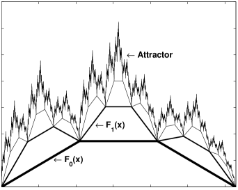
Figure 2: Formation of the FIF attractor after successive iterations

1.2 Discrete FIF

One of the most interesting properties of the FIF is that its attractor is independent of the initial signal (initiator). If the initiator is a continuous signal, for example the linear interpolation between the given interpolation points, all the instances throughout all the steps of the iterations will be continuous signals, fig. 2. On the other hand if the initiator is a single point the attractor formed after infinite iterations will be a continuous signal, but signals instances of the FIF throughout the iterations will be discrete signals, fig. 3. Although during all the iterations the instances are discrete signals or strictly mathematically speaking finite countable sets, the attractor is a continuous signal, an infinite and uncountable set. Instances of a the formation of an FIF from a discrete initiator are shown in fig. 3.

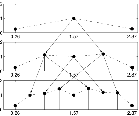
Figure 3: Generation of a discrete FIF.

It is essential to show that a good choice of the initiator is the $N+1$ given interpolation points $(x_{n},y_{n}),n=0,1\dots N$. After the first iteration in each of the $N$ subintervals between the points, $N-2$ new points are generated fig. 3. Let these points be $(x_{s},y_{s}),s=1,\dots,(N-1)N$. Notice that all these $N+1+(N-2)N=N^{2}-N+1$ points belong to the attractor of FIF. This wouldn’t be true if the initiator was a different set apart from the given interpolation points. By repeating this procedure after $m$ iterations we get an $M(m)$-point discrete sequence that is a sampling of the FIF’s attractor, with sampling period $T_{s}=\frac{1}{M}$. If the initiator included any other irrelevant point, that would not be mapped to an attractor’s point after a finite number of iterations. It can be proved that if the initiator is not the set of the initial interpolation points, then the error of the formed sequence after the $m$th iteration from the attractor decreases and goes to zero as $m\rightarrow\infty$. The number of the attractor’s samples is :

$$N+1$$

$$N+1+(N-1)N = N^{2}+1$$

$$N+1+(N-1)N+(N-1)N^{2} = N^{3}+1$$

$$\vdots \vdots$$

$$M=M(m)=N^{m}+1.$$ (6)

The discrete signal formed after the $m$th iteration over the discrete initiator, is called discrete FIF :

$$f[n]=F(x_{n}),\quad n=0,1,\dots,M$$ (7)

Before expanding Barnsley operator ${\mathcal{T}}$ introduced above for the discrete FIF it is necessary to make clear that according to the strict definition of Fractals the discrete FIFs are not fractal sets because they are finite. Discrete FIFs must be considered as approximations of the continuous.

Since the Barnsley operator assumes infinite resolution, it doesn’t apply in discrete signals. So for discrete FIF the following modified operator is used:

$${\mathcal{T}}f[n]=\sum_{k=1}^{N}(d_{k}{\uparrow}^{N}f[\frac{n-e_{k}}{a}] +c_{k}(\frac{n-e_{k}}{a})+f_{n})$$ (8)

$$(u(n-e_{k-1})-u(n-e_{k})).$$

The Symbol ${\uparrow}^{N}f[n]$ defines that within two successive samples of $f[n]$, $N-1$ zeros have been interpolated, fig. 4. The term $f_{n}$ denotes the parameter of FIF as defined in (5) and should not be confused with the discrete signal $f[n]$.

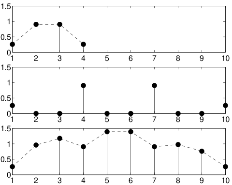
Figure 4: Barnsley operator for discrete signals. The initiator is upsampled and interpolated according to (1.2

Similarly to the continuous case, a discrete FIF of m iterations can be constructed with the following procedure:

$$f_{m+1}[n]={\mathcal{T}}f_{m}[n].$$ (9)

It is obvious that when $m\rightarrow\infty$ the discrete FIF becomes continuous. Notice that ${\mathcal{T}}$ depends on the number of iterations $m$. More specifically the parameters of FIF as defined in (2-5) depend on the $x_{n}$. The $x_{n}$ change value because of the upsampling. The generation of an FIF can be represented in terms of a linear system as shown in fig. 5.

Figure 5: Block diagram of the FIF Genaration.

2 Computation of FIF’s Fourier Spectrum

In order to simplify (2-5), it is very convenient to adopt the following assumptions.

• $x_{0}=0,\quad x_{N}=1,$

• $F_{0}=F_{N}=0.$

• and the points are evenly spaced.

Then(2-5) becomes,

$$a_{n} = \frac{1}{N},$$ (10)

$$e_{n} = \frac{n-1}{N},$$ (11)

$$c_{n} = F_{n}-F_{n-1},$$ (12)

$$f_{n} = F_{n-1}.$$ (13)

The above equations show that the FIF parameters are decoupled from each other. This is very important because they can be estimated independently. Moreover it is clear that if $a_{n}$ parameter is estimated then all parameters can be found directly, except for $d_{n}$.

Any FIF can be transformed to an equivalent FIF that satisfies the first two conditions without loosing its fundamental properties. More specifically fig. 6 shows how a given FIF can be transformed so as to satisfy the conditions for the first and the last point. It is convenient to use an auxiliary affine map $w_{aux}$ that will rotate, scale and translate the given one. The $w_{aux}$ transform is invertible and does not affect the intrinsic parameters $a_{n},d_{n}$.

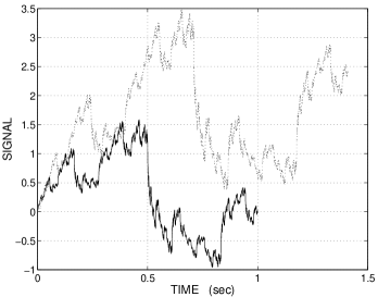
Figure 6: An example of FIF out of range $[0,1]$. Applying an affine transform we can tie it at points $(0,0)$ and $(1,0)$.

Let $A=\{(x,y):F(x)=y\},$ be the original attractor and

$${\bigcup}_{n=1}^{N}w_{n}(A)=A$$ (14)

where $w_{n}$,

$$w_{n}\left[\begin{array}[]{c}x\\ y\end{array}\right]=\left[\begin{array}[]{cc}a_{n}&0\\ c_{n}&d_{n}\end{array}\right]\left[\begin{array}[]{c}x\\ y\end{array}\right]+\left[\begin{array}[]{c}e_{n}\\ f_{n}\end{array}\right],n=1,\dots,N$$

The new transformed attractor is $A^{\prime}=\{(x^{\prime},y^{\prime}),F^{\prime}(x)=y^{\prime}\}.$ The new points are connected with the initial

$$\left[\begin{array}[]{c}x^{\prime}\\ y^{\prime}\end{array}\right]=\left[\begin{array}[]{cc}a_{aux}&0\\ c_{aux}&d_{aux}\end{array}\right]\left[\begin{array}[]{c}x\\ y\end{array}\right]+\left[\begin{array}[]{c}e_{aux}\\ f_{aux}\end{array}\right]$$

That means $A^{\prime}=w_{aux}A$. These new points belong to a new FIF. Setting in (14) $A=w^{-1}_{aux}A^{\prime}$ and applying the map $w_{aux}$,

$${\bigcup}_{n=1}^{N}w_{aux}w_{n}w^{-1}_{aux}(A^{\prime})=A^{\prime},$$ (15)

with

$$w^{-1}_{aux}=\left[\begin{array}[]{cc}1/a_{aux}&0\\ -\frac{c_{aux}}{a_{aux}d_{aux}}&1/d_{aux}\end{array}\right].$$

By setting $f_{aux}=e_{aux}=0,$ $d_{aux}=1$, the affine maps of the new FIF are :

$$w^{\prime}_{n}\left[\begin{array}[]{c}x^{\prime}\\ y^{\prime}\end{array}\right]=\left[\begin{array}[]{cc}a_{n}&0\\ (c_{n}-d_{n}c_{aux}+c_{aux}a_{n})/a_{aux}&d_{n}\end{array}\right]$$ (20)

$$\left[\begin{array}[]{c}x^{\prime}\\ y^{\prime}\end{array}\right]+\left[\begin{array}[]{c}a_{aux}e_{n}\\ c_{aux}e_{n}+f_{n}\end{array}\right]$$ (25)

Notice that the new FIF has the same order and the same $d_{n}$ parameters.

2.1 Spectrum of Continuous FIF

The application of the above simplifications to the Barnsley operator $T$ results in the following equation for the FIF:

$$\begin{array}[]{l}F(x)=\sum_{n=1}^{N}(d_{n}F(\frac{x-e_{n}}{a})+\\ +c_{n}(\frac{x-e_{n}}{a})+f_{n})(u(x-e_{n-1})-u(x-e_{n}))\end{array}$$ (26)

and

$$u(x)=\left\{\begin{array}[]{ll}0&\mbox{$x<0$}\\ 1&\mbox{$x\geq 0$}\end{array}\right.$$

$G(x)$ is the piecewise linear function between the interpolation points :

$$G(x)=\sum_{n=1}^{N}c_{n}(\frac{x-e_{n}}{a}+f_{n})(u(x-e_{n-1})-u(x-e_{n})).$$

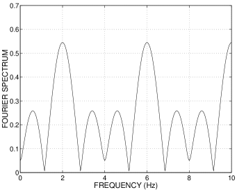
Figure 7: An example of ${\mathcal{Q}}(\Omega)$.

Applying continuous fourier transform [5]:

$${\mathcal{F}}(\Omega)=\int_{-\infty}^{+\infty}F(x)e^{-i\Omega x}dx$$

$$F(x) \longleftrightarrow {\mathcal{F}}(\Omega)$$

$${\mathcal{F}}(\Omega) = {\mathcal{G}}(\Omega)+a{\mathcal{F}}(a\Omega)\sum_{n=1}^{N}d_{n}e^{-i\Omega e_{n}},$$ (27)

$$\begin{array}[]{l}{\mathcal{G}}(\Omega)=\sum_{n=1}^{N}(\frac{e^{-i\Omega\frac{n-1}{N}}-e^{-i\Omega\frac{n}{N}}}{(i\Omega)^{2}}(\frac{c_{n}}{a}+i\Omega(f_{n}-\frac{c_{n}e_{n}}{a}))\\ +\frac{c_{n}}{a}\frac{\frac{n-1}{N}e^{-i\Omega\frac{n-1}{N}}-\frac{n}{N}e^{-i\Omega\frac{n}{N}}}{i\Omega})\end{array}$$ (28)

We define the function :

$${\mathcal{Q}}(\Omega)=a\sum_{n=1}^{N}d_{n}e^{-i\Omega\frac{(n-1)}{N}}=a\sum_{n=0}^{N-1}d_{n+1}e^{-i\frac{\Omega n}{N}}$$ (29)

Notice that the above function is the discrete time fourier transform of the discrete sequence $\{d_{1},d_{2},\dots d_{N}\}$, so we deduce that $Q(\Omega-2k\pi N)=Q(2(k+1)\pi N-\Omega),\quad k=1,2,\dots\quad$ (fig. 7).

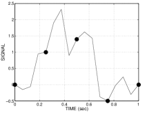
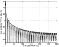
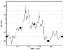
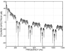
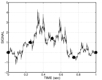
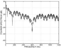
Figure 8: Left column: Fractal interpolation between points $(0,0),(0.25,1),(0.5,1.4),(0.75,-0.5),(1,0)$ after 1,3,5 iterations. right column: Corresponding spectrums.

The Fourier spectrum satisfies the following equation:

$${\mathcal{F}}(\Omega)={\mathcal{Q}}(\Omega){\mathcal{F}}(a\Omega)+{\mathcal{G}}(\Omega)$$ (30)

Through Barsley Operator in frequency domain the Fourier spectrum can be computed iteratively, fig. 8.

$${\mathcal{F}}_{m+1}(\Omega)={\mathcal{Q}}(\Omega){\mathcal{F}}_{m}(a\Omega)+{\mathcal{G}}(\Omega)$$ (31)

${\mathcal{F}}_{0}(\Omega)=0.$
After infinite iterations:

$${\mathcal{F}}(\Omega)=\sum_{i=0}^{\infty}{\mathcal{G}}(\Omega a^{i})\prod_{j=0}^{i-1}{\mathcal{Q}}(\Omega a^{j})$$ (32)

2.2 Spectrum of Discrete FIF

From the (32) it is obvious that the FIF signals are not band-limited. As a result the spectrum of a discrete FIF is aliased. Assume $T_{s}=\frac{1}{M}$ has been chosen as the sampling period, then the Discrete Time Fourier Transform (DTFT) [5] is :

$${\hat{f}}(\omega)=\sum_{n=0}^{M}f[n]e^{-i\omega n},\omega=\Omega T_{s}.$$

As in continuous case for the computation of the DTFT the ${\mathcal{T}}$ operator is used in frequency domain:

$$\hat{f}_{m+1}(\omega)=\hat{f}_{m}(a\omega)\sum_{p=1}^{N}d_{k}ae^{-i\omega e_{p}}+\hat{g}_{m}(\omega)$$ (33)

Posing the analogy between the continuous and the discrete case we define the $q$ function :

$$\hat{q}_{m}(\omega)=a\sum_{p=1}^{N}d_{p}e^{-i\omega e_{p}}.$$

$$\hat{q}(\omega)=\sum_{p=1}^{N}d_{p}e^{-i{\omega}e_{p}},\quad p=0,1,\dots,N.$$

and $e_{p}=\frac{p-1}{N}(M-1),$ so

$$\begin{array}[]{l}{\hat{q}}(\omega)=\sum_{p=0}^{N-1}d_{p+1}e^{\frac{-i{\omega}p}{N}(M-1)}\\ =\sum_{p=0}^{N-1}d_{p+1}e^{(-i{\omega}p)(N^{m-1}-\sum_{i=1}^{m-2}N^{i})},\quad p=0,1,\dots,N.\end{array}$$ (34)

$${\hat{f}}_{m+1}(\omega)={\hat{q}}_{m}(\omega){\hat{f}}_{m}(a\omega)+{\hat{g}}_{m}(\omega)$$ (35)

After $m$ iterations

$${\hat{f}}_{m}(\omega)=\sum_{i=0}^{m}{\hat{g}}_{m-i}(\omega a^{i})\prod_{j=0}^{i-1}{\hat{q}}_{i-j+1}(\omega a^{j})\\$$ (36)

The Discrete Fourier Transform can be computed after keeping the frequency values between $0$ and $2\pi$ and sampling the spectrum at $\omega=0,\frac{2\pi}{M},2\frac{2\pi}{M},\dots,(M-1)\frac{2\pi}{M}$ , fig. 9.

In the continuous case ${\mathcal{Q}}(\Omega)$ has period $2\pi N$. In the discrete case where ${\omega}\in[0,2\pi]$ the ${\hat{q}}(\omega)$ function has period $2\pi\frac{N}{M-1}$.

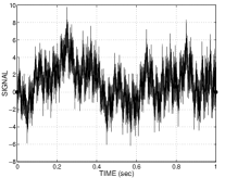
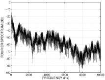
Figure 9: 5-point FIF attractor with $d_{n}=-0.74,0.8,-0.77,0.85,0.88.$ and the spectrum after the 5th iteration.

3 FIF parameter estimation using spectrum

FIF modelling of signals has been proposed by Mazel [3], using information of signal in time domain. In this section the spectrum of signal is used to estimate its parameters, provided the FIF order is known.

Given the signal $f[n],n=0,1,\dots,M$ , let $N$ be FIF’s estimated order. We expect its spectrum to satisfy the following equation:

$${\hat{q}}[\omega_{k}]=\frac{{\hat{f}}_{m+1}[\omega_{k}]-{\hat{g}}[\omega_{k}]}{{\hat{f}}_{m}[a\omega_{k}]},$$

$$\quad a\omega_{k}=0,\frac{2\pi}{MN},2\frac{2\pi}{MN},\dots,(MN-1)\frac{2\pi}{MN}.$$

All values that zero denominator are excluded. Notice that $f_{m+1}[n]$ and $f_{m}[n]$ signals must have the same length. Considering also that $f_{m+1}[0]=f_{m}[0]$ and $f_{m+1}[M(m+1)]=f_{m}[M(m)]$, where $M(m),M(m+1)$ their lengths. In order to equalize their lengths it is necessary to interpolate with zeros $f_{m}[n]$. Because of the term ${\hat{f}}_{m}[a\omega_{k}]$ the computation of FFT must be on $\frac{2k\pi}{MN},k=0,\dots,NM-1$. This is done by padding the signal with $MN-M$ zeros. The $d_{n}$ are determined by the solution of the system of linear equations.

$$\left[\begin{array}[]{c}\hat{q}(0)\\ \hat{q}[\omega_{1}]\\ \hat{q}[\omega_{2}]\\ \vdots\\ \hat{q}[\omega_{N}]\end{array}\right]=\left[\begin{array}[]{ccccc}1&1&\dots&1\\ 1&e^{\frac{-i\omega_{1}}{N}}&\dots&e^{\frac{-(N-1)i\omega_{1}}{N}}\\ 1&e^{\frac{-i\omega_{2}}{N}}&\dots&e^{\frac{-(N-1)i\omega_{2}}{N}}\\ \vdots&\vdots&\dots&\vdots\\ 1&e^{\frac{-i\omega_{R}}{N}}&\dots&e^{\frac{-(N-1)i\omega_{R}}{N}}\\ \end{array}\right]\left[\begin{array}[]{c}d_{1}\\ d_{2}\\ d_{3}\\ \vdots\\ d_{N}\end{array}\right]$$ (37)

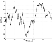
(a)

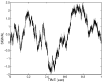
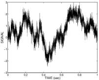
(b) (c)

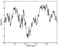
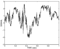
(d) (e)

Figure 10: (a) FIF without noise. In (b),(c) FIF contaminated with noise $\mathit{SNR}=20$ and $\mathit{SNR}=10$. In (d),(e) reconstructed FIF.

4 Results

The above algorithm was tested in FIF signals contaminated with white noise and the parameters extracted were very close to the real, fig. 10. The main advantage of the method is the use of FFT. It is well known that FFT is quite simple and easily implemented. The first disadvantage of the method is that it cannot find the FIF order. In the above experiments we tried for $N=2,3,\dots$ until the estimated ${\hat{q}}$ function satisfied the periodicity and symmetry conditions mentioned earlier. The second and most important problem is that it is very sensitive in the window effect of the FFT. It is known that although a part of FIF signal is self affine it is not an FIF. Trying to model it as an FIF results in wrong estimations. In the example of fig. 11, it is evident that the period of the ${\hat{q}}$ function has been expanded. Having chosen the order $N$, the period of ${\hat{q}}$ is known $2\pi\frac{N}{M-1}$. In the right plot of fig. 11 it is evident that the period of ${\hat{q}}$ is much higher than the expected. But although the spectrum is not the best method for solving the inverse problem it can be used as powerful analysis tool. As shown above it can reveal the FIF nature of a signal and it can also help in the prediction of a missing part of a time series, given that it belongs to class of FIF.

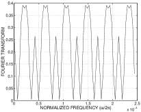
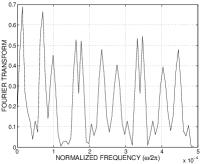
Figure 11: Left : $\hat{q}(\omega)$. Right : $\hat{q}(\omega)$ of the corrupted FIF.

References

[1] B. B. Mandelbrot, ”The Fractal Geometry of Nature”
W.H Freeman and Company, New York, 1983.
[2] M. F. Barnsley,
”Fractals Everywhere”,
Academic Press, 1993.
[3] D. S. Mazel, M. H. Hayes,
”Using Iterated Function Systems to Model Discrete Sequences”,
IEEE Transactions on Signal Processing, Vol. 40 (7), pp. 1724-1734, July 1992.
[4] H. D.I. Abarbanel,
”Analysis of Observed Chaotic Data”,
Springer Verlag, New York 1996.
[5] A. V.Oppenheim, R. W. Schafer,
”Deiscrete-Time Signal Processing”,
Prentice Hall, 1999.
(a)
(a) (b)
(b)
(c)
(c) (d)
(d)
(e)
(e)