Imitating quantum mechanics: qubit-based model for simulation

Abstract

We present an approach to simulating quantum computation based on a classical model that directly imitates discrete quantum systems. Qubits are represented as harmonic functions in a 2D vector space. Multiplication of qubit representations of different frequencies results in exponential growth of the state space similar to the tensor-product composition of qubit spaces in quantum mechanics. Individual qubits remain accessible in a composite system, which is represented as a complex function of a single variable, though entanglement imposes a demand on resources that scales exponentially with the number of entangled qubits. We carry out a simulation of Shor’s algorithm and discuss a simpler implementation in this classical model.

I Introduction

Quantum computation promises exponential speed-up over classical computation for certain problems, such as period finding and quantum simulation. Traditional classical simulation of a composite quantum system requires updating each of the $2^{N}$ amplitudes characterizing the state of $N$ qubits, according to a Hamiltonian made up of $2^{N}\times 2^{N}$ elements. The exponential growth of the state space with $N$ imposes a severe burden on resources for this type of simulation. Finding classes of quantum computations that can be simulated efficiently is an active field of research tensor .

In quantum mechanics, the qubits that comprise a composite system remain accessible, and it is through interactions with individual and pairs of qubits that computation is implemented. For example, a single-qubit transformation affects all $2^{N}$ computational basis states of an $N$-qubit system. It therefore seems that one of the features of quantum systems that enables more efficient computing is the ability to harness the degrees of freedom of a $2^{N}$D vector space by interacting with only $N$ qubits.

Here we present a classical model of discrete quantum systems that is based on representing individual qubits and transformations applied to them. This enables us to address specific qubits in a composite system, the state of which is represented as a complex function of a single variable, and thereby directly replicate the steps in an algorithm as they would be implemented in a quantum system. While the resources required to carry out a computation exactly are comparable to other methods, this model may be compatible with new approximations that would enable simulating more qubits than currently is feasible. Furthermore, the approach of building a classical model based on imitating quantum systems could offer an opportunity to gain insight into the difference in computational power of classical and quantum architectures.

II Review of Quantum Computation

A qubit can be realized with any two-state quantum system that can be prepared in a general superposition of basis states of a 2D, complex vector space. For multiple uncoupled qubits, the state of the composite system is given by the tensor product of the individual states, and the number of computational basis states grows exponentially with the number of qubits. For example, the state of an $N$-qubit system, with each qubit in an equal superposition of computational basis states $|0\rangle$ and $|1\rangle$, is given by the state vector,

$$|\Psi\rangle = \left(\frac{1}{\sqrt{2}}\right)^{N}\big{(}|0\rangle+|1\rangle\big{)}_{1}\otimes\big{(}|0\rangle+|1\rangle\big{)}_{2}\otimes$$ (1)

$$\hskip 54.2025pt\big{(}|0\rangle+|1\rangle\big{)}_{3}\otimes\ldots\otimes\big{(}|0\rangle+|1\rangle\big{)}_{N}$$

$$= \left(\frac{1}{\sqrt{2}}\right)^{N}\big{(}|00...00\rangle+|00...01\rangle+$$

$$\hskip 68.65627pt|00...10\rangle+\ldots+|11...11\rangle\big{)}.$$

Application of a unitary operation to a qubit that is part of a composite system, which constitutes a step in an algorithm, affects all states in the superposition simultaneously, illustrating the massive parallelism inherent in quantum computation.

Any quantum algorithm can be approximated arbitrarily closely using just single qubit operations and a generic two-qubit interaction, such as the controlled-NOT (CNOT) gate universal . The effects of these operations can be visualized as rotations and inversions of the $2^{N}$–dimensional quantum-computer state vector. The state in Eq. (1), constructed as a product of individual qubit states, is a special case. Almost all of the states the system can occupy in its vector space will be non-separable, implying that entanglement is required for general computation.

Qubits and operations on them are subject to perturbations from the environment and experimental imperfections. In general, it is believed that errors due to decoherence grow exponentially with the number of qubits in a system decoherence . Realizable quantum computation relies on the ability to diminish the effects of these errors–quantum error correction and fault-tolerant quantum computation exploit entanglement and the discrete nature of quantum systems to make this possible.

This brief introduction to the fundamental elements of quantum computation emphasizes the role played by the mathematical structure of the single- and multiple-qubit vector spaces. Quantum systems require this mathematical description, and our classical model is developed according to this description by building into it the same state-space structure. The result is a new method of simulation and an architecture that may offer insight into the fundamental advantages of quantum systems for computing.

III Individual Qubits

For the representation of a qubit we use a harmonic function with frequency $\omega$. Orthogonal functions $\sin(\omega t)$ and $\cos(\omega t)$ serve as convenient basis states and span a 2D vector space. We assign these basis functions the role of the computational basis states of a qubit,

$$|0\rangle \Longleftrightarrow \sin(\omega t)$$

$$|1\rangle \Longleftrightarrow \cos(\omega t).$$ (2)

Applying a general unitary transformation $U$ to a qubit $\psi$,

$$\psi(t)=\alpha\sin(\omega t)+\beta\cos(\omega t),$$ (3)

requires isolating the coefficients $\alpha$ and $\beta$; each coefficient can then be multiplied by the corresponding transformed basis function, yielding the transformed state:

$$U\big{[}\psi(t)\big{]}=\alpha\hskip 1.4457ptU\big{[}\sin(\omega t)\big{]}+\beta\hskip 1.4457ptU\big{[}\cos(\omega t)\big{]}.$$ (4)

Orthogonality of the basis functions makes it straightforward to isolate the coefficients by taking the inner product of the corresponding function with $\psi(t)$:

$$\alpha=\frac{\omega}{\pi}\int_{0}^{2\pi/\omega}\sin(\omega t^{\prime})\psi(t^{\prime})~{}dt^{\prime},$$

$$\beta=\frac{\omega}{\pi}\int_{0}^{2\pi/\omega}\cos(\omega t^{\prime})\psi(t^{\prime})~{}dt^{\prime}.$$ (5)

A general transformation is illustrated in Fig. 1(a).

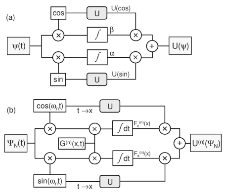
Figure 1: Schematic showing a linear transformation on single and multi-qubit states. (a) For a single qubit, orthogonality of the basis functions enables isolation of the coefficients, which can then be multiplied by the transformed basis functions. (b) For a composite system, the generator $G^{(n)}(x,t)$ enables the functional form of $F^{(n)}(t)$ to be transferred to a different variable. This procedure is analogous to addressing a qubit in a quantum system.

The modulus squared of the coefficient, or amplitude, of a basis function gives the corresponding “measurement probability”. The function representing a qubit can be replaced with one or the other basis function according to these probabilities in order to represent the measurement process. The ability to determine both measurement probabilities for a given state eliminates the need to introduce and carry along normalization coefficients–the relative probabilities can be determined at the time of measurement.

IV Composite Systems

IV.1 $2^{N}$D Vector Space

This model can be extended to composite systems by using a different frequency for the basis functions for each two-state system, creating a new 2D vector space for each qubit. The mapping of quantum states to functions for composite systems becomes

$$|0\rangle_{n} \Longleftrightarrow \sin(\omega_{n}t)$$

$$|1\rangle_{n} \Longleftrightarrow \cos(\omega_{n}t),~{}~{}~{}n=0,1,...,N-1,$$ (6)

where $n$ refers to the $n$th qubit and $N$ is the total number in the system.

If $N$ single-qubit functions in equal superpositions are multiplied, the result is a linear combination of $2^{N}$ different products,

$$\Psi_{N}(t) = \big{(}\sin(\omega_{1}t)+\cos(\omega_{1}t)\big{)}\big{(}\sin(\omega_{2}t)+\cos(\omega_{2}t)\big{)}\ldots\big{(}\sin(\omega_{N}t)+\cos(\omega_{N}t)\big{)}$$

$$= \big{(}\sin(\omega_{1}t)\sin(\omega_{2}t)\ldots\sin(\omega_{N}t)\big{)}+\big{(}\sin(\omega_{1}t)\sin(\omega_{2}t)\ldots\cos(\omega_{N}t)\big{)}+\ldots$$

$$+\big{(}\cos(\omega_{1}t)\cos(\omega_{2}t)\ldots\cos(\omega_{N}t)\big{)}.$$

This is analogous to the tensor-product state for a composite quantum system in Eq. (1), with the mapping

$$|b_{1}b_{2}b_{3}\ldots b_{N}\rangle \Leftrightarrow h_{1}(\omega_{1}t)h_{2}(\omega_{2}t)h_{3}(\omega_{3}t)\ldots h_{N}(\omega_{N}t)$$ (8)

$$\equiv H_{N,j}(t).$$

Here, $b_{n}$ is the binary value representing the state of the $n$th qubit of a quantum system, $h_{n}$ is the basis function (sine or cosine) representing the $n$th qubit in our model, and $H_{N,j}(t)$ is the $j$th of the $2^{N}$ combinations of products of $h_{n}$.

The functions $H_{N}(t)$ that naturally arise when representing composite systems look like $N$-qubit computational basis states, and we would like to determine whether they too span a state space that grows exponentially with qubit number. This will be the case if all of the $2^{N}$ functions are orthogonal. It is easy to see by expanding the products of harmonic functions in terms of sum and difference frequencies that, for $N$ qubits, the $H_{N}(t)$ are comprised of $2^{N-1}$ Fourier frequencies $\Omega_{l}=\sum_{n=1}^{N}\sigma_{l,n}\omega_{n}$, where $\sigma_{l,n}$ is 1 or $-1$. The $\Omega_{l}$ are all multiples of a fundamental frequency given by the greatest common divisor of the qubit frequencies, $\Omega_{\rm fund}={\rm gcd}(\omega_{1},\omega_{2},\ldots,\omega_{N})$ bezout . The orthogonality of the individual Fourier components can be shown to lead to orthogonality of the $H_{N}(t)$ for few qubits; the three-qubit case is demonstrated in Appendix A.

IV.1.1 Orthogonality of the $H_{N}(t)$

To demonstrate orthogonality in the general case when the $2^{N-1}$ Fourier frequencies are unique, we consider the inner product between two $N$-qubit functions $H_{N,j}(t)=h_{j,1}(\omega_{1}t)\ldots h_{j,N}(\omega_{N}t)$ and $H_{N,k}(t)=h_{k,1}(\omega_{1}t)\ldots h_{k,N}(\omega_{N}t)$,

$$H_{N,j}(t)\cdot H_{N,k}(t)\propto\int_{0}^{\pi/\Omega_{\rm fund}}\Big{[}h_{j,1}(\omega_{1}t)h_{k,1}(\omega_{1}t)\Big{]}\Big{[}h_{j,2}(\omega_{2}t)h_{k,2}(\omega_{2}t)\Big{]}\ldots$$

$$\Big{[}h_{j,N}(\omega_{N}t)h_{k,N}(\omega_{N}t)\Big{]}dt,$$ (9)

where factors for a given qubit have been grouped together int_limit . Each product $h_{j,n}(\omega_{n}t)h_{k,n}(\omega_{n}t)$ can be written as a function of frequency $2\omega_{n}$, as either $\frac{1}{2}\sin(2\omega_{n}t)$ or $\frac{1}{2}(1\pm\cos(2\omega_{n}t))$. The integrand in Eq. (9) can then be seen to consist of three types of terms. First, there will always be a term that is a product of a function for each qubit, $h_{1}(2\omega_{1}t)\ldots h_{N}(2\omega_{N}t)$. This can be written as a sum of Fourier components with frequencies that are twice those of the $H_{N}(t)$ and are, therefore, also multiples of $\Omega_{\rm fund}$. Because integration of a harmonic function over an integral multiple of its period yields zero, this term’s contribution to the inner product $H_{N,j}(t)\cdot H_{N,k}(t)$ vanishes.

Second, there can be terms that only include factors for some qubits, such as $h_{1}(2\omega_{1}t)\ldots h_{n-1}(2\omega_{n-1}t)h_{n+1}(2\omega_{n+1}t)\ldots h_{N}(2\omega_{N}t)$, which arises when $h_{j,n}=h_{k,n}$. The Fourier frequencies for these terms are also multiples of $\Omega_{\rm fund}$–the fundamental frequency is the greatest common divisor of the set of all qubit frequencies, and necessarily divides any subset of them. These terms therefore also vanish when integrated over an interval of $2\pi/\Omega_{\rm fund}$.

Finally, the integrand in Eq. (9) can have a term of unity (times $1/2^{N}$). This only occurs when all qubit functions are the same for $H_{N,j}(t)$ and $H_{N,k}(t)$, i.e. $H_{N,j}(t)=H_{N,k}(t)$.

IV.1.2 Redundant Frequencies

This argument is only valid if all of the Fourier frequencies $\Omega_{l}$ are unique. If there are at least two combinations of qubit frequencies that give the same Fourier frequency, we can write $\sum_{n=1}^{N}\sigma_{n,l}\omega_{n}=\sum_{n=1}^{N}\sigma_{n,m}\omega_{n}$, for $\Omega_{l}=\Omega_{m}$. Terms that enter this equation with the same sign for each Fourier frequency cancel, and the remaining terms give $\omega_{a}+\omega_{b}+\ldots=\omega_{\alpha}+\omega_{\beta}+\ldots$, where the frequencies have been arranged so that all signs are positive. When considering all inner products $H_{N,j}(t)\cdot H_{N,k}(t)$, all possible combinations of harmonic factors in the integrand in Eq. (9) will arise; for some inner product, there will be a term in the integrand like $h(2\omega_{a}t)h(2\omega_{b}t)\ldots h(2\omega_{\alpha}t)h(2\omega_{\beta}t)\ldots$, with Fourier frequencies that include $\Omega=2(\omega_{a}+\omega_{b}+\ldots-\omega_{\alpha}-\omega_{\beta}-\ldots)=0$. For the case(s) in which this frequency is the argument of a cosine, the constant term results in a nonzero integral, and the different $H_{N}(t)$ in this case are not orthogonal.

Therefore, for sets of qubit frequencies $\{\omega_{n}\}$ that result in $2^{N-1}$ unique Fourier frequencies, the functions $H_{N}(t)$ that naturally arise when representing composite systems are orthogonal and span a $2^{N}$–dimensional space. Unique Fourier frequencies can be ensured by using a qubit-frequency definition such as $\omega_{n}=\omega/2^{n-1}$.

IV.2 Linear Operations

In quantum computation, single-qubit operations along with a generic two-qubit interaction, such as a CNOT gate, are universal. The general approach to implementing operations in our model of composite quantum systems is the same as for a single qubit–we need to isolate the factor multiplying each basis function ($\sin(\omega_{n}t)$ or $\cos(\omega_{n}t)$) for a particular qubit. In this case, these factors will be expressions involving other qubit basis functions. Once isolated, they can be multiplied by the transformed basis functions and these recombined to generate the transformed composite function.

Consider a general $\Psi_{N}(t)$, similar to Eq. (IV.1) but with arbitrary coefficients for the $H_{N}(t)$. We can write $\Psi_{N}$ as a sum of two parts, one with terms that include $\cos(\omega_{n}t)$ and one with terms that include $\sin(\omega_{n}t)$:

$$\Psi_{N}(t) = \bigg{(}\sum_{k=1}^{2^{N-1}}a_{k}H_{k,N}^{(n)}(t)\bigg{)}\cos(\omega_{n}t)+\bigg{(}\sum_{k=1}^{2^{N-1}}b_{k}H_{k,N}^{(n)}(t)\bigg{)}\sin(\omega_{n}t)$$ (10)

$$= F_{c}^{(n)}(t)\cos(\omega_{n}t)+F_{s}^{(n)}(t)\sin(\omega_{n}t).$$

The $H_{k,N}^{(n)}(t)$ are products of harmonic functions,

$$h_{1}(\omega_{1}t)h_{2}(\omega_{2}t)\ldots h_{n-1}(\omega_{n-1}t)h_{n+1}(\omega_{n+1}t)\ldots h_{N}(\omega_{N}t),$$

where $h$ is cosine or sine, and $a_{k}$, $b_{k}$ are coefficients for the $\cos(\omega_{n}t)$, $\sin(\omega_{n}t)$ terms. $F_{c}^{(n)}(t)$ and $F_{s}^{(n)}(t)$ are the functions that we need to be able to isolate to apply a linear transformation to qubit $n$; determining these functions can be considered to be “addressing qubit $n$.”

For small $N$, a procedure similar to the one for a single qubit can be adapted. Multiplication of $\Psi_{N}$ by the relevant basis function for the qubit leads to a different spectrum for terms containing that basis function. These different frequencies could be selected from the terms containing the orthogonal basis function, enabling the qubit to be addressed. As the qubit number grows, however, the number and density of frequencies grow dramatically, making this process unfeasible.

A more general procedure can be used which determines $F_{c}^{(n)}~{}\big{(}F_{s}^{(n)}\big{)}$ exactly using the orthogonality of the $H_{N}(t)$. An inner product can be imposed between $\Psi_{N}$ and a projector that forces all of the terms with one basis function for qubit $n$ to vanish while preserving the others. The construction of the projector for a given system is straightforward.

A linear combination of all of the $H_{N}(t)$ for a system of $N$ qubits can be generated by putting each qubit into an equal superposition of basis functions as in Eq. (IV.1). We define a similar function, the generator for qubit $n$, as the product of equal superpositions of computational basis states for all qubits in the system except qubit $n$:

$$G_{N}^{(n)}(t)=\big{(}\sin(\omega_{1}t)+\cos(\omega_{1}t)\big{)}\big{(}\sin(\omega_{2}t)+\cos(\omega_{2}t)\big{)}\ldots\big{(}\sin(\omega_{n-1}t)+\cos(\omega_{n-1}t)\big{)}$$

$$\big{(}\sin(\omega_{n+1}t)+\cos(\omega_{n+1}t)\big{)}\ldots\big{(}\sin(\omega_{N}t)+\cos(\omega_{N}t)\big{)}.\hskip 54.2025pt$$ (11)

If this is multiplied by $\cos(\omega_{n}t)~{}\big{(}\sin(\omega_{n}t)\big{)}$, the resulting function’s inner product with $\Psi_{N}(t)$ gives the sum of the amplitudes of the terms in $F_{c}^{(n)}(t)~{}\big{(}F_{s}^{(n)}(t)\big{)}$, but the functional form is lost. We can salvage the functional dependence by transferring it to a second variable introduced to exactly replicate the dependence on $t$:

$$G_{N}^{(n)}(x,t)=\hskip 325.215pt$$

$$\big{(}\sin(\omega_{1}t)\sin(\omega_{1}x)+\cos(\omega_{1}t)\cos(\omega_{1}x)\big{)}\big{(}\sin(\omega_{2}t)\sin(\omega_{2}x)+\cos(\omega_{2}t)\cos(\omega_{2}x)\big{)}\ldots$$

$$\big{(}\sin(\omega_{n-1}t)\sin(\omega_{n-1}x)+\cos(\omega_{n-1}t)\cos(\omega_{n-1}x)\big{)}\big{(}\sin(\omega_{n+1}t)\sin(\omega_{n+1}x)\hskip 36.135pt$$

$$+\cos(\omega_{n+1}t)\cos(\omega_{n+1}x)\big{)}\ldots\big{(}\sin(\omega_{N}t)\sin(\omega_{N}x)+\cos(\omega_{N}t)\cos(\omega_{N}x)\big{)}\hskip 14.45377pt$$

$$=\cos(\omega_{1}t-\omega_{1}x)\cos(\omega_{2}t-\omega_{2}x)\ldots\cos(\omega_{n-1}t-\omega_{n-1}x)\ldots\hskip 54.2025pt$$

$$\cos(\omega_{n+1}t-\omega_{n+1}x)\ldots\cos(\omega_{N}t-\omega_{N}x).$$ (12)

When this generator is multiplied by $\cos(\omega_{n}t)~{}(\sin(\omega_{n}t))$, we get the projector for $F_{c}^{(n)}(t)~{}\big{(}F_{s}^{(n)}(t)\big{)}$:

$$P_{c}^{(n)}(x,t) = \cos(\omega_{n}t)~{}G_{N}^{(n)}(x,t)$$

$$\Big{(}P_{s}^{(n)}(x,t) = \sin(\omega_{n}t)~{}G_{N}^{(n)}(x,t)\Big{)}.$$ (13)

Taking the inner product of $\Psi_{N}(t)$ and $P_{c}^{(n)}(x,t)~{}\big{(}P_{s}^{(n)}(x,t)\big{)}$, integrated over $t$, gives us $F_{c}^{(n)}(x)~{}\big{(}F_{s}^{(n)}(x)\big{)}$:

$$F_{c}^{(n)}(x) = (2^{N}\Omega_{\rm fund}/\pi)\int_{0}^{\pi/\Omega_{\rm fund}}P_{c}^{(n)}(x,t)\Psi_{N}(t)~{}dt$$

$$\Big{(}F_{s}^{(n)}(x) = (2^{N}\Omega_{\rm fund}/\pi)\int_{0}^{\pi/\Omega_{\rm fund}}P_{s}^{(n)}(x,t)\Psi_{N}(t)~{}dt\Big{)}.$$ (14)

This is an exact technique for addressing a qubit that is part of a composite system. The rest of the procedure for applying a transformation follows as in the single-qubit case and is illustrated in Fig. 1(b).

Iteration of this technique of addressing qubits allows for multiple-qubit gates. For example, for a controlled-NOT gate with qubit $n_{1}$ as the control and $n_{2}$ as the target, the gate would begin with determination of $F_{c}^{(n_{1})}$, which would then take on the role of the function $\Psi$ for determining $F_{c}^{(n_{2})}$ and $F_{s}^{(n_{2})}$. $F_{c}^{(n_{1})}$ would be reconstructed after inverting the basis functions for $n_{2}$, giving $F_{c}^{(n_{2})}(t)\sin(\omega_{2}t)+F_{s}^{(n_{2})}(t)\cos(\omega_{2}t)$. Finally, the transformed state would be generated as $\Big{(}F_{c}^{(n_{2})}(t)\sin(\omega_{2}t)+F_{s}^{(n_{2})}(t)\cos(\omega_{2}t)\Big{)}\cos(\omega_{1}t)+F_{s}^{(n_{1})}(t)\sin(\omega_{1}t)$. Gates involving more than two qubits can be implemented by further iteration.

The measurement probability for a basis function is determined by $\int_{0}^{\pi/\Omega_{\rm fund}}F^{(n)\ast}(t)\cdot F^{(n)}(t)~{}dt$ meas_prob . Due to the orthogonality of the $H_{N}(t)$, all cross terms in the inner product vanish and the result is the sum of the moduli squared of the amplitudes of all of the terms containing the corresponding basis function.

IV.3 Scaling of Required Resources

The state of a general composite system can be represented as

$$\Psi(\omega_{1},\omega_{2},...,\omega_{N_{e}})\psi(\omega_{N_{e}+1})\psi(\omega_{N_{e}+2})\ldots,$$ (15)

where $\psi$ represents an individual, unentangled qubit, and $\Psi$ characterizes $N_{e}$ entangled qubits. While unentangled qubits can be stored and processed individually and with little overhead, the resources required to exactly represent entangled qubits scale exponentially with $N_{e}$ clusters . The qubit frequencies and the maximum Fourier frequency can be kept finite, but the fundamental frequency decreases at least exponentially with number. The interval over which $\Psi$ needs to be defined is given by the integration interval required for addressing a qubit. In Eq. (14), the integration limit of $\pi/\Omega_{\rm fund}$ yields exact values for the $F^{(n)}$; coupled with the necessary resolution imposed by the highest Fourier frequency, on order of $\Omega_{\rm max}/\Omega_{\rm fund}$ points are required to define $\Psi$.

We can consider the impact on addressing a qubit–both for a unitary transformation and for measurement–of simply truncating all of the functions that arise in a calculation. For unitary transformations, we determine the accuracy of $F_{c}^{(n)}(\tau,t)$ and $F_{s}^{(n)}(\tau,t)$, the functions determined by integrating Eq. (14) to $\tau$ rather than to $\pi/\Omega_{\rm fund}$, by comparing $F_{c}^{(n)}(\tau,t)\cos(\omega_{n}t)+F_{s}^{(n)}(\tau,t)\sin(\omega_{n}t)$ to $\Psi(t)$. We define a parameter $\delta^{(n)}(\tau)$ to represent the error in $F^{(n)}(\tau,t)$:

$$\delta^{(n)}(\tau)=\int_{0}^{\tau}\Big{(}\tilde{\Psi}(x)-\frac{1}{\rm N(\tau)}\Big{[}\Big{(}\int_{0}^{\tau}P_{c}^{(n)}(x,t)\tilde{\Psi}(t)~{}dt\Big{)}\cos(\omega_{n}x)\hskip 72.26999pt$$

$$+\Big{(}\int_{0}^{\tau}P_{s}^{(n)}(x,t)\tilde{\Psi}(t)~{}dt\Big{)}\sin(\omega_{n}x)\Big{]}\Big{)}^{2}dx,$$ (16)

where $\tilde{\Psi}$ is $\Psi$ normalized over the interval 0 to $\tau$, and N$(\tau)$ is the normalization constant for $F_{c}^{(n)}(\tau,t)\cos(\omega_{n}t)+F_{s}^{(n)}(\tau,t)\sin(\omega_{n}t)$ over the same interval.

In Fig. 2(a) we plot $\delta(\tau)$ for the state $\Psi(t)=\prod_{n=1}^{N_{e}}\cos(\omega_{n}t)+\prod_{n=1}^{N_{e}}\sin(\omega_{n}t)$, with $\omega_{n}=\omega/2^{n-1}$ and $N_{e}=5$ through 9. We evaluate $\delta$ for the case of addressing the first qubit. The curves show that determination of $F_{c}^{(n)}$ and $F_{s}^{(n)}$, which is exact for an integration limit of $\pi/\Omega_{\rm fund}$, abruptly becomes less precise as the integration interval is reduced. Any calculation involving many gates will likely require a value for $\delta$ on the steep part of the curve, imposing an integration interval that scales exponentially with $N_{e}$.

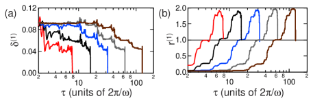
Figure 2: (Color online.) (a) Semi-log plot of error $\delta$ versus integration time $\tau$ when addressing qubit $n=1$ for the state discussed in the text. The equal spacing between the steep parts of the curves indicates an exponential scaling of integration interval in order to avoid significant errors. (b) Plot of $r$ versus integration time $\tau$, for the same state and addressing the same qubit. For both plots, curves from left to right correspond to $N_{e}=5,6,7,8$ and 9 qubits, and each curve extends to $\pi/\Omega_{\rm fund}$ for the corresponding $N_{e}$.

To assess the effect of truncation on measurement probabilities, we truncate the integrals used to determine $F_{c}^{(n)}$ and $F_{s}^{(n)}$ as above, and then integrate the square of each. We look at the ratio of the truncated probability to measure sine versus cosine as a function of integration time:

$$r^{(n)}(\tau)=\int_{0}^{\tau}\Big{(}\int_{0}^{\tau}P_{s}^{(n)}(x,t)\Psi(t)~{}dt\Big{)}^{2}~{}dx\Big{/}\int_{0}^{\tau}\Big{(}\int_{0}^{\tau}P_{c}^{(n)}(x,t)\Psi(t)~{}dt\Big{)}^{2}~{}dx.$$ (17)

This ratio is plotted in Fig. 2(b) for the same state used above, for which the actual ratio is one. The graph shows that reaching the actual ratio of $P_{s}$ to $P_{c}$ also scales exponentially with $N_{e}$. However, precise values for measurement probabilities are often not needed and useful qualitative information can be obtained for integration intervals that are shorter than $\pi/\Omega_{\rm fund}$. For instance, for this example the curves indicate that for integration limits beyond $\pi/(4\hskip 1.4457pt\Omega_{\rm fund})$, the ratio $r$ is about 0.25, of the same order as the actual value.

V Simulation Example–Factoring

V.1 The Quantum Fourier Transform and Shor’s Algorithm

The most celebrated quantum algorithm is Shor’s method of finding the prime factors of a number N. The problem of factorization can be related to the problem of determining the period $p$ of the function $f(x)=a^{x}({\rm mod}~{}\textsf{N})$, for an integer $a$ that is co-prime with N; if $p$ is even, either $(a^{p/2}+1)$ or $(a^{p/2}-1)$ will have a common factor with N mermin_shor . Shor’s algorithm relies on application of the quantum Fourier transform (QFT) to $f(x)$ to efficiently determine the period.

The qubits involved in implementing this algorithm are divided into two registers, the states of which are treated as integers according to the states of the associated qubits. The first step in the procedure is to prepare the first register in a superposition of all computational basis states,

$$\sum_{x=0}^{2^{N_{1}}-1}|x\rangle,$$

by applying a Hadamard transform to each of the $N_{1}$ qubits in the register norm . A gate $U$ applied to both registers produces the entangled state

$$\sum_{x=0}^{2^{N_{1}}-1}|x\rangle\otimes|a^{x}({\rm mod}~{}\textsf{N})\rangle.$$ (18)

If the second register is measured, it collapses to $|a^{x_{0}}({\rm mod}~{}\textsf{N})\rangle$ for some $x_{0}$. The first register ends up in a superposition of all states $|x^{\prime}\rangle$ for which $a^{x^{\prime}}({\rm mod}~{}\textsf{N})=a^{x_{0}}({\rm mod}~{}\textsf{N})$, leaving the system in the state

$$\big{(}|x_{0}\rangle+|x_{0}+p\rangle+|x_{0}+2p\rangle+\ldots\big{)}\otimes|a^{x_{0}}({\rm mod}~{}\textsf{N})\rangle.$$ (19)

Application of the QFT to the first register imposes interference that results in a superposition of states $|\tilde{x}\rangle$ that are close to integral multiples of the inverse period, $\tilde{x}\approx\tilde{x}_{\kappa}=\kappa(2^{N_{1}}/p),$ for integer $\kappa$. Measurement yields an integer close to one of the $\tilde{x}_{\kappa}$, and after several iterations the period $p$ can be determined.

The minimum number of qubits required for each register is $N_{1}=\log_{2}\textsf{N}^{2}$ and $N_{2}=\log_{2}\textsf{N}$. This ensures that the second register is large enough to represent $p$, which satisfies $p\leq\textsf{N}$, and that the first register is large enough to give a unique value for $p$ from the QFT (see reference mermin_shor ). We apply our model to the factorization of $\textsf{N}=21$ using $a=2$, the first integer co-prime with 21. This requires 14 qubits, nine for the first register and five for the second; the alogorithm for our example is illustrated in Fig. 3. The qubits are labeled 1 through 14, with the convention that qubit 1 (14) is the most (least) significant qubit for the first (second) register. Qubit $n$ is represented using the frequency $\omega_{n}=\omega/2^{n-1}$, and the function $\Psi$ representing the state of the system is defined with a resolution of $1/\omega$ over an interval of $2\pi/\Omega_{\rm fund}=2\pi(2^{n_{\rm max}-1})$ resolution . In Fig. 4 we show the function representing the state of the system at various stages in the calculation, as denoted by the dashed lines in Fig. 3(a).

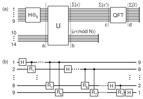
Figure 3: (a) Illustration of Shor’s factoring algorithm for $\textsf{N}=21$. The first gate shown represents an application of the Hadamard transform to each of the nine qubits in the first register. The solid vertical lines that terminate the circuit flow represent measurement; the dashed vertical lines indicate points at which $\Psi$ is plotted in Fig. 4. (b) Circuit for implementing the quantum Fourier transform shown in (a). The unitary gate $R_{d}$ is a rotation by the angle $\pi/2^{d}$, and $H$ is a Hadamard transform. The QFT reverses the order of the qubits.

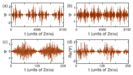
Figure 4: (Color online.) Function $\Psi$ representing the state of the system at various stages in the simulation, plotted over one period. The different durations shown are due to the different number of qubits at those points in the calculation. Only the real part of the function is plotted in (d).

We implement $U$ by generating the output state, shown in Fig. 4(b), by summing all functions representing $|x\rangle|a^{x}({\rm mod}~{}\textsf{N})\rangle$ over $x=0$ to $x=2^{14}-1$ qubit_burden . From here, we measure qubits 10 through 14 by comparing $F_{s}^{(n)\ast}\cdot F_{s}^{(n)}$ to $F_{c}^{(n)\ast}\cdot F_{c}^{(n)}$ and applying the rule that the outcome of a measurement is the state with the higher measurement probability, or is chosen at random if the probabilities are equal. This leaves the second register in the state $|10000\rangle=|16\rangle$, and the first register in a linear combination of all $|x^{\prime}\rangle$ between 0 and $2^{9}-1$ for which $2^{x^{\prime}}({\rm mod}~{}21)=16$; the function representing the first register at this stage is shown in Fig 4(c). Qubits 10 through 14 are removed from the calculation and the QFT is applied to the remaining nine qubits.

The results of applying the QFT and subsequent measurement of qubits 1–9 are shown in Fig. 5(a), which displays the measurement probability for the state $|\tilde{x}\rangle$. The peaks at multiples of $85\frac{1}{3}$ indicate a period of $p=6$ for the function $2^{x}({\rm mod}~{}21)$, which in turn yields either of the prime factors of 21 from ${\rm gcd}(a^{p/2}+1,\textsf{N})$ and ${\rm gcd}(a^{p/2}-1,\textsf{N})$. Figures 5(b)-(d) zoom in on the probability distributions near different multiples of $85\frac{1}{3}$. When $\kappa\times 85\frac{1}{3}$ is not an integer, the probability is distributed among integers closest to the fractional value, as in (b) and (c).

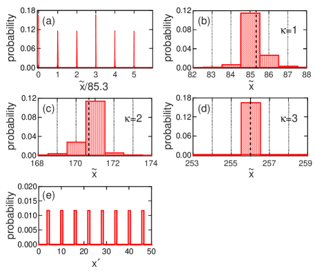
Figure 5: (Color online.) Results of the QFT applied to the first register. (a) Plot of measurement probability for all $\tilde{x}$ between 0 and 511. The six peaks are designated by the integer $\kappa=0$ through 5. (b)–(d) Details of peaks for $\kappa=1,2$ and 3 in (a). The dashed line indicates the exact value of $\kappa(2^{N_{1}}/p)$ for that peak. (e) Plot of measurement probability versus $x^{\prime}$ for the case when the QFT is not used. Only part of the entire distribution, which extends to $x^{\prime}=511$, is shown.

V.2 Simplifications in a Classical Model

There is a dramatic simplification to the factoring algorithm when using a classical model for simulation. The need for the QFT stems from the fact that, in a quantum system, measurement of the state in Eq. (19) results in one of the states in the superposition, with no opportunity to learn the others. Repetition of the algorithm to that point likely results in a different $x_{0}$, preventing the period from being learned in successive iterations. In a classical system, the state in Eq. (19) can be measured as many times as necessary to determine the period $p$. If we apply this simplified scheme to the state $\Psi$ in Fig. 4(c), we find equal probability for any $x^{\prime}$ satisfying $2^{x^{\prime}}({\rm mod}~{}21)=16$; the first eight peaks are shown in Fig. 5(e).

In addition to avoiding all of the gates required for the QFT, no imaginary numbers are required, and most importantly, we save on qubits. The first register, whose size for Shor’s algorithm is dictated by the QFT stage, in this case only needs enough qubits to represent $p$, and $p\leq\textsf{N}$. This provides a savings on order of $\log_{2}\textsf{N}$ qubits compared to the quantum case. Applying this simplified factoring algorithm to $N=21$ would require only 10 qubits, five for each register.

VI Conclusion

We have presented a classical, qubit-based model of discrete quantum systems that offers a new framework for simulating quantum computations by providing access to individual qubits and their interactions. The dimension of the state space for a composite system grows exponentially with qubit number, and individual qubits continue to be accessible. Application to Shor’s algorithm highlights the features of the model in action. The resources required for implementation scale exponentially with the number of entangled qubits, yet it is possible to save on qubits in a classical model.

Appendix A Fourier Decomposition of $H_{N}(t)$

The $H_{N}(t)$ can be Fourier decomposed by expanding the products of harmonics $h_{n}$ in terms of sum and difference frequencies. Here we explicitly show the decomposition for the case of 3 qubits. The 8 functions $H_{3,j=1\ldots 8}(t)$ can be expanded as

$$\cos(\omega_{1}t)\cos(\omega_{2}t)\cos(\omega_{3}t)=\frac{1}{4}\Big{(}\cos\big{[}(\omega_{1}+\omega_{2}+\omega_{3})t\big{]}+\cos\big{[}(\omega_{1}+\omega_{2}-\omega_{3})t\big{]}$$

$$+\cos\big{[}(\omega_{1}-\omega_{2}+\omega_{3})t\big{]}+\cos\big{[}(\omega_{1}-\omega_{2}-\omega_{3})t\big{]}\Big{)}$$

$$\cos(\omega_{1}t)\cos(\omega_{2}t)\sin(\omega_{3}t)=\frac{1}{4}\Big{(}\sin\big{[}(\omega_{1}+\omega_{2}+\omega_{3})t\big{]}-\sin\big{[}(\omega_{1}+\omega_{2}-\omega_{3})t\big{]}$$

$$+\sin\big{[}(\omega_{1}-\omega_{2}+\omega_{3})t\big{]}-\sin\big{[}(\omega_{1}-\omega_{2}-\omega_{3})t\big{]}\Big{)}$$

$$\cos(\omega_{1}t)\sin(\omega_{2}t)\cos(\omega_{3}t)=\frac{1}{4}\Big{(}\sin\big{[}(\omega_{1}+\omega_{2}+\omega_{3})t\big{]}+\sin\big{[}(\omega_{1}+\omega_{2}-\omega_{3})t\big{]}$$

$$-\sin\big{[}(\omega_{1}-\omega_{2}+\omega_{3})t\big{]}-\sin\big{[}(\omega_{1}-\omega_{2}-\omega_{3})t\big{]}\Big{)}$$

$$\cos(\omega_{1}t)\sin(\omega_{2}t)\sin(\omega_{3}t)=\frac{1}{4}\Big{(}-\cos\big{[}(\omega_{1}+\omega_{2}+\omega_{3})t\big{]}+\cos\big{[}(\omega_{1}+\omega_{2}-\omega_{3})t\big{]}$$

$$+\cos\big{[}(\omega_{1}-\omega_{2}+\omega_{3})t\big{]}-\cos\big{[}(\omega_{1}-\omega_{2}-\omega_{3})t\big{]}\Big{)}$$

$$\sin(\omega_{1}t)\cos(\omega_{2}t)\cos(\omega_{3}t)=\frac{1}{4}\Big{(}\sin\big{[}(\omega_{1}+\omega_{2}+\omega_{3})t\big{]}+\sin\big{[}(\omega_{1}+\omega_{2}-\omega_{3})t\big{]}$$

$$+\sin\big{[}(\omega_{1}-\omega_{2}+\omega_{3})t\big{]}+\sin\big{[}(\omega_{1}-\omega_{2}-\omega_{3})t\big{]}\Big{)}$$

$$\sin(\omega_{1}t)\cos(\omega_{2}t)\sin(\omega_{3}t)=\frac{1}{4}\Big{(}-\cos\big{[}(\omega_{1}+\omega_{2}+\omega_{3})t\big{]}+\cos\big{[}(\omega_{1}+\omega_{2}-\omega_{3})t\big{]}$$

$$-\cos\big{[}(\omega_{1}-\omega_{2}+\omega_{3})t\big{]}+\cos\big{[}(\omega_{1}-\omega_{2}-\omega_{3})t\big{]}\Big{)}$$

$$\sin(\omega_{1}t)\sin(\omega_{2}t)\cos(\omega_{3}t)=\frac{1}{4}\Big{(}-\cos\big{[}(\omega_{1}+\omega_{2}+\omega_{3})t\big{]}-\cos\big{[}(\omega_{1}+\omega_{2}-\omega_{3})t\big{]}$$

$$+\cos\big{[}(\omega_{1}-\omega_{2}+\omega_{3})t\big{]}+\cos\big{[}(\omega_{1}-\omega_{2}-\omega_{3})t\big{]}\Big{)}$$

$$\sin(\omega_{1}t)\sin(\omega_{2}t)\sin(\omega_{3}t)=\frac{1}{4}\Big{(}-\sin\big{[}(\omega_{1}+\omega_{2}+\omega_{3})t\big{]}+\sin\big{[}(\omega_{1}+\omega_{2}-\omega_{3})t\big{]}$$

$$+\sin\big{[}(\omega_{1}-\omega_{2}+\omega_{3})t\big{]}-\sin\big{[}(\omega_{1}-\omega_{2}-\omega_{3})t\big{]}\Big{)}.$$ (20)

We introduce a more compact notation to represent the 8 Fourier components:

$$(1,0,0,0,0,0,0,0) \equiv \frac{1}{4}\cos\left((\omega_{1}+\omega_{2}+\omega_{3})t\right)$$

$$(0,1,0,0,0,0,0,0) \equiv \frac{1}{4}\cos\left((\omega_{1}+\omega_{2}-\omega_{3})t\right)$$

$$(0,0,1,0,0,0,0,0) \equiv \frac{1}{4}\cos\left((\omega_{1}-\omega_{2}+\omega_{3})t\right)$$

$$(0,0,0,1,0,0,0,0) \equiv \frac{1}{4}\cos\left((\omega_{1}-\omega_{2}-\omega_{3})t\right)$$

$$(0,0,0,0,1,0,0,0) \equiv \frac{1}{4}\sin\left((\omega_{1}+\omega_{2}+\omega_{3})t\right)$$

$$(0,0,0,0,0,1,0,0) \equiv \frac{1}{4}\sin\left((\omega_{1}+\omega_{2}-\omega_{3})t\right)$$

$$(0,0,0,0,0,0,1,0) \equiv \frac{1}{4}\sin\left((\omega_{1}-\omega_{2}+\omega_{3})t\right)$$

$$(0,0,0,0,0,0,0,1) \equiv \frac{1}{4}\sin\left((\omega_{1}-\omega_{2}-\omega_{3})t\right).$$ (21)

For all of these terms, $(1_{a})\cdot(1_{b})=\delta_{ab}(\pi/16\hskip 1.4457pt\Omega_{\rm fund})$, where $(1_{a})$ corresponds to the Fourier component represented by the row vector with a one in the $a$th place and zeros everywhere else.

The functions $H_{3}(t)$ written with this vector notation become

$$\cos(\omega_{1}t)\cos(\omega_{2}t)\cos(\omega_{3}t) = (1,1,1,1,0,0,0,0)$$

$$\cos(\omega_{1}t)\cos(\omega_{2}t)\sin(\omega_{3}t) = (0,0,0,0,1,-1,1,-1)$$

$$\cos(\omega_{1}t)\sin(\omega_{2}t)\cos(\omega_{3}t) = (0,0,0,0,1,1,-1,-1)$$

$$\cos(\omega_{1}t)\sin(\omega_{2}t)\sin(\omega_{3}t) = (-1,1,1,-1,0,0,0,0)$$

$$\sin(\omega_{1}t)\cos(\omega_{2}t)\cos(\omega_{3}t) = (0,0,0,0,1,1,1,1)$$

$$\sin(\omega_{1}t)\cos(\omega_{2}t)\sin(\omega_{3}t) = (-1,1,-1,1,0,0,0,0)$$

$$\sin(\omega_{1}t)\sin(\omega_{2}t)\cos(\omega_{3}t) = (-1,-1,1,1,0,0,0,0)$$

$$\sin(\omega_{1}t)\sin(\omega_{2}t)\sin(\omega_{3}t) = (0,0,0,0,-1,1,1,-1).$$

From this it can be seen that all of the $H_{3}(t)$ are orthogonal. For example,

$$\cos(\omega_{1}t)\cos(\omega_{2}t)\cos(\omega_{3}t)\cdot\cos(\omega_{1}t)\sin(\omega_{2}t)\sin(\omega_{3}t)=$$

$$(1,1,1,1,0,0,0,0)\cdot(-1,1,1,-1,0,0,0,0)=\hskip 13.00806pt$$

$$-1+1+1-1=0.\hskip 86.72377pt$$ (22)

In this case and for small numbers of qubits, all of the different inner products can be verified to be zero, and $H_{N,j}\cdot H_{N,j}=(\pi/4\hskip 1.4457pt\Omega_{\rm fund})$.

We can also see that not all of the functions are orthogonal if there is redundancy in the Fourier frequencies. If, for instance, $\omega_{1}+\omega_{2}-\omega_{3}=\omega_{1}-\omega_{2}+\omega_{3}$, then the second and third vectors in Eq. (21) are identical (as are the sixth and seventh). In this case, the $H_{3}(t)$ can only be represented by six orthogonal vectors, not eight. Then,

$$\cos(\omega_{1}t)\cos(\omega_{2}t)\cos(\omega_{3}t)\cdot\cos(\omega_{1}t)\sin(\omega_{2}t)\sin(\omega_{3}t)=$$

$$(1,2,1,0,0,0)\cdot(-1,2,-1,0,0,0)=\hskip 13.00806pt$$

$$-1+4-1=2.\hskip 86.72377pt$$ (23)

References

- (1) See, for example, G. Vidal, Phys. Rev. Lett., 91, 147902 (2003).
- (2) D. Deutsch, A. Barenco, and A. Ekert, Proc. R. Soc. London, Ser. A 449, 669 (1995).
- (3) G. M. Palma, K.-A. Suominen, and A. K. Ekert, Proc. R. Soc. London, Ser. A 452, 567 (1996).
- (4) This can be seen using Bézout’s identity.
- (5) Typially, the integration limit in this equation should be . Because frequencies are always doubled in this and similar expressions, we can use as the integration limit.
- (6) Because we do not carry along normalization coefficients, these inner products for the two basis functions are compared to determine relative measurement probabilites.
- (7) Clearly, if there are several subsets of entangled qubits with no entanglement between subsets, then each collection would be described by its own , and resources would scale exponentially only with the number within a subset.
- (8) A nice description of the details of Shor’s algorithm can be found in N. David Mermin, “Some curious facts about quantum factoring,” Physics Today, October 2007, p. 10.
- (9) In the discussion of this algorithm, we use the common practice of describing transformations applied to registers as opposed to individual qubits, and we omit all normalization factors.
- (10) The maximum Fourier frequency is , so the shortest period is ; choosing a resolution of satisfies the Nyquist sampling criterion.
- (11) The general method of imposing via controlled modular exponentiation requires a minimum of additional qubits quantum_arithmetic , which is too computationally burdensome at this stage of the calculation.
- (12) V. Vedral, A. Barenco, and A. Ekert, Phys. Rev. A, 54, 147 (1996).