Towards measurable bounds on entanglement measures

Abstract

While the experimental detection of entanglement provides already quite a difficult task, experimental quantification of entanglement is even more challenging, and has not yet been studied thoroughly. In this paper we discuss several issues concerning bounds on concurrence measurable collectively on copies of a given quantum state. Firstly, we concentrate on the recent bound on concurrence by Mintert–Buchleitner [F. Mintert and A. Buchleitner, Phys. Rev. Lett. 98, 140505 (2007)]. Relating it to the reduction criterion for separability we provide yet another proof of the bound and point out some possibilities following from the proof which could lead to improvement of the bound. Then, relating concurrence to the generalized robustness of entanglement, we provide a method allowing for construction of lower bounds on concurrence from any positive map (not only the reduction one). All these quantities can be measured as mean values of some two–copy observables. In this sense the method generalizes the Mintert–Buchleitner bound and recovers it when the reduction map is used. As a particular case we investigate the bound obtained from the transposition map. Interestingly, comparison with MB bound performed on the class of $4\otimes 4$ rotationally invariant states shows that the new bound is positive in regions in which the MB bound gives zero. Finally, we provide measurable upper bounds on the whole class of concurrences.

I Introduction

Entanglement review-horo is the property of quantum states of multipartite systems that is absolutely crucial for the future emerging quantum technologies: from quantum communication, through quantum information, to quantum metrology and quantum sensing roadmap . For this reason there has been a considerable interest in the recent years in designing feasible and efficient methods of entanglement detection (see the recent review on this subject GuhneToth ). Particularly important in this respect are entanglement detection schemes which require only local measurements of the entangled parts of the composite system. Among the most important approaches to local entanglement detection the following methods are perhaps the most popular and useful:

• Quantum state tomography. This method employs very many local measurements, and becomes impractical in higher dimensions. It is very useful for low dimensional systems, where frequently entanglement criteria for the states in question are known white98 ; blatt1 ; blatt2 .

• Entanglement visibility methods. These require detection of only some elements of the density matrix, but for a continuous family of measuring devices settings (cf. visibility ).

• Bell’s tests. These methods do more than just a check of entanglement - they check also the non–locality of the quantum states Bell . Obviously, they do not detect the entangled states that do not violate any Bell inequality Werner ; lhv (see also the review reviewbell ).

• Entanglement witnesses (EW). These are observables that have positive averages on all separable states, but a negative one on at least one entangled state horo96 ; terhal . They can be measured locally, and one can optimize such measurements in various aspects guehnepra . Nowadays, entanglement witnesses are routinely used in experiments to detect entanglement (see e.g. Refs. blatt1 ; demartini ; harald ).

• ”Direct” entanglement detection schemes. Such schemes have been proposed for pure huelga ; Walborn or mixed states PHConc ; MintertBuchleitner ; RAMDPH . Particularly interesting are those using structural approximations of positive maps PHorodecki_From ; pawel_ekert ; korbiczpra .

• Nonlinear entanglement witnesses. Such objects involve measurement of several copies typically. Examples are discussed, e.g., in Refs. PHorodecki_From ; guehne1 . There are related methods employing measurements of variances guehne2 or higher order correlation functions blatt2 ; korbicz , or even entropic uncertainty relations Takeuchi ; guehne3 ; Julio_entr .

With the exception of quantum tomography (which tries to get all possible information about the state, but is very costly in resources), all of the above listed methods aim at answering the qualitative question: given a state, is it entangled? Only in few instances, these methods allow for further characterization of different classes of entanglement, and various kinds of optimization. For example, EWs allow to distinguish different classes of multipartite entanglement (cf. acin3 ). Optimization of EWs may concern their effectiveness (amount of states detected), or the complexity of experimental implementation hyllus .

While, the qualitative entanglement detection problem is already quite difficult and complex, it is even more challenging and practically important to pose the quantitative question: given a state, how much entangled it is?. For this aim one has to use entanglement measures (EM). There are many of those (see e.g. Refs. Michal-measures ; Plenio-measures ), and there is no canonical choice. Various measures are more, or less useful, depending on the physical and quantum informational context.

Entanglement measures are typically non measurable directly. Having chosen an EM, one needs reliable bounds on it, that can be then directly measured experimentally (see Ref. MintertAPB ). The new emerging area of quantitative entanglement detection consists thus to a great extend in the search for efficient and measurable bounds for EM s. This area is the subject of this paper.

Recently, there were several other papers dealing with the problem of efficient bounds on entanglement measures. Let us just recall some of these achievements. One of the earliest results in this area comes from Breuer BreuerBound , who provided a lower bound on concurrence employing a mean value of some particular linear EW. Other interesting bound for concurrence of this sort was proposed in the bipartite case by Mintert and Buchleitner MintertBuchleitner (see also Ref. Mintert for the bound in a more general fashion) and then generalized to the multipartite scenario in Ref. Aolita . Also, ”dual” upper bounds for concurrence in both the bipartite and multipartite scenarios were provided in Ref. Guo . Interestingly, all these bounds are measurable collectively on two copies of a state and the Mintert–Buchleitner (MB) bound was even very recently measured Schmid (see also Ref. Bovino for another experiment and Jaksch1 for proposal of an experiment in the multipartite scenario both aiming at determination of the same quantities, however, in purely qualitative context and also recent criticism on these kinds of experiments Enk1 ; Enk2 ). Let us finally mention that the general approach to derivation of bounds for various entanglement measures from an incomplete information about the state (coming from the knowledge of averages of certain observables) was recently worked out in a series of papers Brandao ; Brandao0 ; Plenio ; Reimpell_1 ; Reimpell_2 ; Eisert ; Wunderlich .

The main purpose of the paper is presentation of a possible generalization of the MB bound. Firstly, however, in Sec. II we make a brief review in which we recall some of the lower and upper bounds on concurrence mentioned above. In particular we concentrate on the bounds measurable on two copies of a state, i.e., those from Refs. MintertBuchleitner ; Mintert ; Guo , however, we recall also the result of BreuerBound . Then, in Sec. IV we provide yet another proof of the Mintert–Buchleitner bound on concurrence. Recently an alternative proof of the MB bound, based on the upper bound on Uhlmann–Jozsa fidelity UhlmannFid ; Jozsa from Ref. Miszczak , was provided in Ref. alternativeProof . Here, utilizing the notion of the conjugate function of concurrence, but also the bound on fidelity, we provide yet another proof of MB bound and its multipartite version from Ref. Aolita . On the one hand, it seems that this approach could give some possibilities of direct improvements of the bound. On the other hand, the present approach allows to relate the MB bound to the reduction map. This connection, in turn, leads to a new method of derivation of lower measurable bounds on concurrence from any positive map (Sec. IV). All the obtained bounds are measurable on two copies of a given state. Moreover, in the particular case of the reduction map the method recovers the MB bound and therefore can be treated as its generalization to the case of arbitrary positive map. Particularly interesting is the transposition map, which is known to be stronger in detection of entanglement than the reduction one. Hence, as checked in the case of $4\otimes 4$ rotationally invariant states, the resulting bound works for states for which the MB bound does not. Unfortunately, surely due to the lack of optimization, the bounding values are in general much lower that the ones of the MB bound.

Further, in Sec. V, we extend a little the result of Ref. Guo showing that the whole class of concurrences discussed in Refs. Sinolecka ; Jap ; Gour may be bounded from above by some measurable functions of the state. In Sec. VI we conclude the paper pointing also out some possibilities for further research.

II Recent lower and upper measurable bounds on concurrence

Before proceeding with detailed considerations let us recall the definition of concurrence both in the bipartite and multipartite scenario. In general, when dealing with the bipartite case we will utilize the so–called $I$–concurrence introduced by Rungta et al. Rungta in an attempt to generalize the Hill–Wootters concurrence Hill . In the multipartite case the extension of $I$–concurrence provided in Ref. Carvalho will be used. We will also recall some of the lower and upper bounds on these concurrences measurable on two copies of a given state, provided so far in the literature.

II.1 Bipartite case

Let us start from the bipartite case. For this purpose let $|\psi_{AB}\rangle$ denote some bipartite pure state from the Hilbert space $\mathcal{H}_{A}\otimes\mathcal{H}_{B}=\mathbbm{C}^{d}\otimes\mathbbm{C}^{d}$. Following Rungta we define $I$–concurrence (hereafter called concurrence) of $|\psi_{AB}\rangle$ as follows

$$C(|\psi_{AB}\rangle) = \sqrt{2\left(1-\mathrm{Tr}\varrho_{r}^{2}\right)}$$

$$= \sqrt{4\sum_{i<j}\mu_{i}^{(r)}\mu_{j}^{(r)}},$$

when $\varrho_{r}$ stands for one of the reductions of $|\psi_{AB}\rangle$, i.e., $\varrho_{r}=\mathrm{Tr}_{A(B)}|\psi_{AB}\rangle\!\langle\psi_{AB}|$ and $0\leq\mu_{i}^{(r)}\leq 1$ are eigenvalues of $\varrho_{r}$ (or squared Schmidt coefficients of $|\psi_{AB}\rangle$). Notice that from the above definition it follows that for the maximally entangled state from $\mathbbm{C}^{d}\otimes\mathbbm{C}^{d}$, i.e.,

$$|\psi_{+}^{(d)}\rangle=\frac{1}{\sqrt{d}}\sum_{i=0}^{d-1}|ii\rangle,$$ (2)

the concurrence (II.1) is given by $C(|\psi_{+}^{(d)}\rangle)=\sqrt{2(d-1)/d}$. The extension of $C$ to all mixed states acting on $\mathcal{H}_{A}\otimes\mathcal{H}_{B}$ is via the convex roof, which means that for any bipartite mixed state $\varrho_{AB}$ one defines concurrence as

$$C(\varrho_{AB})=\min_{\{p_{i},|\psi_{AB}^{(i)}\rangle\}}\sum_{i}p_{i}C(|\psi_{AB}^{(i)}\rangle),$$ (3)

where the minimum is taken over all such ensembles $\{p_{i},|\psi_{AB}^{(i)}\rangle\}$ that $\varrho_{AB}=\sum_{i}p_{i}|\psi_{AB}^{(i)}\rangle\!\langle\psi_{AB}^{(i)}|$.

Having recalled the definition of concurrence we may pass to the lower bound provided in Ref. MintertBuchleitner (from now on we shall be omitting the subscripts $AB$). It was shown there that the concurrence obeys the following inequality

$$C^{2}(\varrho)\geq 2\max_{r=A,B}\left\{\mathrm{Tr}\varrho^{2}-\mathrm{Tr}\varrho_{r}^{2}\right\}.$$ (4)

In the case when the right–hand side is negative we put zero.

This result was further extended in Ref. Mintert , where a more general inequality for concurrence was shown, namely, for any pair of bipartite density matrices $\varrho$ and $\sigma$ it holds that

$$C(\varrho)C(\sigma)\geq 2\max_{r=A,B}\{\mathrm{Tr}\varrho\sigma-\mathrm{Tr}\varrho_{r}\sigma_{r}\}.$$ (5)

For $\sigma=\varrho$ one recovers inequality (4). What is important and interesting about the bound (4) or more generally about the bound (5) is that both can be determined as a mean value of some joint observable on the state $\varrho\otimes\sigma$ (two copies of $\varrho$ in the case of (4). More precisely, the bound (5) can be rewritten as MintertBuchleitner ; Mintert :

$$C(\varrho)C(\sigma)\geq\max_{r=1,2}\left\{\mathrm{Tr}\left(W_{r}\varrho\otimes\sigma\right)\right\},$$ (6)

where $W_{1}=4(P_{-}^{AA^{\prime}}-P_{+}^{AA^{\prime}})\otimes P_{-}^{BB^{\prime}}$ and $W_{2}=4P_{-}^{AA^{\prime}}\otimes(P_{-}^{BB^{\prime}}-P_{+}^{BB^{\prime}})$. Here and in what follows by $P_{+}$ and $P_{-}$ we denote projectors onto symmetric and antisymmetric subspace of the product finite–dimensional Hilbert space $\mathcal{H}\otimes\mathcal{H}$, respectively, which are given by $(1/2)(\mathbbm{1}_{d^{2}}\pm V^{(2)})$. Also, $\mathbbm{1}_{d}$ denotes a $d\times d$ unity matrix and $V^{(2)}$ stands for the so–called swap operator, that is, operator acting as $V^{(2)}|\varphi_{1}\rangle|\varphi_{2}\rangle=|\varphi_{2}\rangle|\varphi_{1}\rangle$ for any pair of $|\varphi_{1}\rangle$ and $|\varphi_{2}\rangle$ from $\mathcal{H}$. Superscripts $AA^{\prime}(BB^{\prime})$ are to indicate on which of subsystems of $\varrho$ and $\sigma$ ($A$ and $B$ are subsystems of $\varrho$ and $A^{\prime}$ and $B^{\prime}$ of $\sigma$) the projectors $P_{\pm}$ act. Interestingly, experiments in which mean values of these observables were achieved have been recently performed Bovino ; Schmid . Note also that the efficiency of the bound (4) was intensively investigated in Ref. Plastino .

Further, upper bound on $C$ ”dual” to the bound (4) and also measurable on two copies of a given state was provided in Ref. Guo , where it was shown that

$$C^{2}(\varrho) \leq 2\min_{r=A,B}\left\{1-\mathrm{Tr}\varrho_{r}^{2}\right\}$$ (7)

$$\equiv \min_{r=1,2}\left\{\mathrm{Tr}\left(\widetilde{W}_{r}\varrho^{\otimes 2}\right)\right\}$$

with $\widetilde{W}_{1}=4P_{-}^{AA^{\prime}}\otimes\mathbbm{1}_{d^{2}}^{BB^{\prime}}$ and $\widetilde{W}_{2}=4\mathbbm{1}_{d^{2}}^{AA^{\prime}}\otimes P_{-}^{BB^{\prime}}$.

Let us now shortly discuss connection of the lower bound on the concurrence (4) to the so–called entropic inequalities introduced firstly in Ref. RHPHMH (see also Ref. RHPH ) as a next example of the so–called scalar separability criteria. The entropic inequalities were further developed in a series of papers MHPH ; Terhal_entr ; VollbrechtWolf . In the most common way they can be written for any separable bipartite state $\varrho$ in the form

$$S_{\alpha}(\varrho)\geq S_{\alpha}(\varrho_{r})\qquad(\alpha\geq 0,\;r=A,B),$$ (8)

where by $S_{\alpha}$ we denoted the quantum Renyi entropy $S_{\alpha}(\rho)=[1/(1-\alpha)]\log\mathrm{Tr}\rho^{\alpha}$. For $\alpha\geq 1$ they simplify to the form $\mathrm{Tr}\varrho_{r}^{\alpha}\geq\mathrm{Tr}\varrho^{\alpha}$ $(r=A,B)$. This, after comparison with Eq. (4) means that the right–hand side of (4) is positive if and only if the entropic inequality (8) with $\alpha=2$ is violated for at least one of subsystems of $\varrho$. In other words, the Mintert–Buchleitner bound works only for states of which entanglement is detected by (8) with $\alpha=2$. However, as it follows e.g. from Refs. Abe ; Tsallis ; Batle (this was also indirectly confirmed in Ref. Plastino ), the efficiency of the entropic inequalities with low $\alpha$s is rather weak and grows significantly with $\alpha\to\infty$. Also, what is particularly important any of the inequalities (8) cannot detect bound entanglement. The latter is a consequence of the fact proven in Ref. VollbrechtWolf that the inequalities (8) follow from the reduction criterion in the sense that if for some $\varrho$ it holds that $(I\otimes R)(\varrho)\geq 0$, then the entropic inequalities (8) are satisfied for all $\alpha$. Here and in what follows by $R$ we denote the so–called reduction map MHPH ; Cerf , which is an example of positive but not completely positive map of the form

$$R(X)=\mathrm{Tr}(X)\mathbbm{1}_{d}-X\qquad(X\in M_{d}(\mathbbm{C})).$$ (9)

The reduction map is decomposable and therefore as such cannot detect PPT entangled states. Consequently, the bound (4) obviously cannot work for PPT entangled states.

On the other hand, as already mentioned, the good think about the entropic inequalities is that as it was confirmed in a series of works (see e.g. Refs. Abe ; Tsallis ; Batle ), they become stronger in detection of entanglement for higher $\alpha$ Therefore it would be interesting to find relations between $C$ or other entanglement measures and the inequalities $\mathrm{Tr}\varrho_{r}^{\alpha}\geq\mathrm{Tr}\varrho^{\alpha}$ for higher $\alpha$s than $2$. Such bounds would be stronger in the sense that they would detect more entangled states and still for integer $\alpha$ would be promising from the experimental point. The latter is because they can be represented as a mean value of some many–copy entanglement witness on $\alpha$ copies of a state $\varrho$ PHorodecki_From . Furthermore, it seems interesting to connect $C$ to recent generalizations of entropic inequalities for all positive maps RAJSPH ; RAJS ; RAJS2 . As the generalized inequalities are able to detect bound entanglement, one could have strong measurable bounds on entanglement measures working also for PPT entangled states.

Let us finally briefly mention other approaches leading to measurable lower bounds on concurrence and in general entanglement measures. First, in Ref. BreuerBound a general bound for the concurrence as a straightforward continuation of the result of Ref. ChenAlbeverioFei (see also Ref. Datta for some extensions of these results). Specifically, it was shown that

$$C(\varrho)\geq\sqrt{\frac{2}{d(d-1)}}\,g(\varrho),$$ (10)

where $g$ is any convex operator function obeying

$$g(|\psi\rangle\!\langle\psi|)\leq 2\sum_{i<j}\sqrt{\mu_{i}\mu_{j}},$$ (11)

for any pure state $|\psi\rangle$ with its Schmidt coefficients $\sqrt{\mu_{i}}$. Examples of functions which satisfy both the conditions and give measurable bounds on concurrence were provided in Refs. BreuerBound ; Julio . In particular, Breuer in BreuerBound considered the function $g_{1}(\varrho)=-\mathrm{Tr}(\varrho W)$ which is convex and showed that for $\mathcal{W}_{\mathcal{V}}=d(I\otimes\Lambda_{\mathcal{V}})(P_{+}^{(d)})$ with $\Lambda_{\mathcal{V}}$ denoting the following positive map introduced in Ref. BreuerMap (see also Ref. Hall for further generalization of this map)

$$\Lambda_{\mathcal{V}}(X)=\mathrm{Tr}(X)\mathbbm{1}_{d}-X-\mathcal{V}X^{T}\mathcal{V}^{\dagger}$$ (12)

with $\mathcal{V}$ standing for unitary antisymmetric (that is $\mathcal{V}^{T}=-\mathcal{V}$) matrix with the only nonzero elements $\pm 1$ lying on its anti–diagonal (see e.g. Ref. BreuerMap ), the function $g_{1}$ also satisfies (11). Specifically, this results in the bound

$$C(\varrho)\geq-\sqrt{\frac{2}{d(d-1)}}\,\mathrm{Tr}\left(\mathcal{W}_{\mathcal{V}}\varrho\right).$$ (13)

Interestingly, in Sec. IV we generalize this inequality to the case of any entanglement witness $W$ satisfying $W\leq\mathbbm{1}_{d}$.

Let us conclude the section by noting that the general method leading to lower bounds on entanglement measures which can be obtained from mean values of some quantum observables was provided recently in a series of papers Brandao ; Brandao0 ; Plenio ; Reimpell_1 ; Reimpell_2 ; Eisert ; Wunderlich .

II.2 Multipartite case

Let us eventually pass to the multipartite scenario. Consider an $N$–partite pure state $|\psi\rangle$ from some finite–dimensional product Hilbert space $\mathcal{H}^{(N)}=\mathcal{H}_{1}\otimes\ldots\otimes\mathcal{H}_{N}$. Then, following Ref. Carvalho we define concurrence of this state as

$$C^{(N)}(|\psi\rangle)=2^{1-N/2}\sqrt{2^{N}-2-\sum_{i}\mathrm{Tr}\varrho_{i}^{2}},$$ (14)

where the sum runs over all subsystems of $|\psi\rangle$ (notice that $|\psi\rangle$ has exactly $2^{N}-2$ proper subsystems). The superscript $N$ is to emphasize that we deal with the multipartite scenario ($C^{(2)}\equiv C$). Again, for mixed state the concurrence $C^{(N)}$ is defined via the convex roof.

Utilizing the bipartite bound (4) it was shown in Ref. Aolita that for any pair of $N$–partite density matrices $\varrho$ and $\sigma$, $C^{(N)}$ satisfies the following inequality

$$C^{(N)}(\varrho)C^{(N)}(\sigma) \geq \frac{4}{2^{N}}\left[\left(2^{N}-2\right)\mathrm{Tr}\varrho\sigma-\sum_{S}\mathrm{Tr}\varrho_{S}\sigma_{S}\right]$$ (15)

$$= \mathrm{Tr}\left(W^{(N)}\varrho\otimes\sigma\right),$$

where the summation runs over all $2^{N}-2$ proper subsystems of $\varrho$ and $\sigma$ (denoted here by $\varrho_{S}$ and $\sigma_{S}$) and

$$W^{(N)}=4\left[\mathbf{P}_{+}-P_{+}^{(1)}\otimes\ldots\otimes P_{+}^{(N)}-\left(1-2^{1-N}\right)\mathbf{P}_{-}\right].$$ (16)

Here $\mathbf{P}_{+}$ ($\mathbf{P}_{-}$) denotes a projector onto symmetric (antisymmetric) subspace of the Hilbert space $\mathcal{H}^{(N)}\otimes\mathcal{H}^{(N)}$, while analogously to the bipartite case, $P_{+}^{(i)}$ $(P_{-}^{(i)})$ stands for a projector onto symmetric (antisymmetric) subspace of $\mathcal{H}_{i}\otimes\mathcal{H}_{i}$, i.e., the Hilbert space representing $i$th particles of $\varrho$ and $\sigma$.

In a similar manner to the bipartite case an upper bound for $C^{(N)}$ dual to the above one (for $\sigma=\varrho$) was proved in Ref. Guo :

$$\left[C^{(N)}(\varrho)\right]^{2} \leq \frac{4}{2^{N}}\left[\left(2^{N}-2\right)-\sum_{S}\mathrm{Tr}\varrho_{S}^{2}\right]$$ (17)

$$= \mathrm{Tr}\left(\widetilde{W}^{(N)}\varrho\otimes\varrho\right)$$

with $\widetilde{W}^{(N)}=W^{(N)}+8(1-2^{1-N})\mathbf{P}_{-}$. It follows straightforwardly from (15) and (17) that both bounds can be measured as mean values of observables $W^{(N)}$ and $\widetilde{W}^{(N)}$, respectively on two copies of $\varrho$ (or $\varrho\otimes\sigma$ in more general case in (15)).

III Proofs of the lower bounds on concurrence

At the very beginning we provide a new proof of the the inequality (5) and in particular the MB inequality (4). For this aim we will utilize the notion of conjugate function (see Refs. ConvexBook ; Audenaert ) of entanglement measures and in particular concurrence (this notion was recently utilized in Refs. Reimpell_1 ; Reimpell_2 ; Eisert to derive measurable bounds on the entanglement measures from mean values of quantum observables) and the very recent upper bound on the fidelity UhlmannFid ; Jozsa proved by Miszczak et al. Miszczak . It has to be emphasized that an alternative proof of the bounds (4) and (5) basing on the latter has been recently provided in Ref. alternativeProof . Here we present a little bit different approach which, in our opinion, could lead, at least in some particular cases, to improvements of the bounds.

Let $E$ denote some entanglement measure, then following Refs. ConvexBook ; Audenaert we define conjugate function of $E$ as

$$\hat{E}(W)=\sup_{\varrho}\left[\mathrm{Tr}(\varrho W)-E(\varrho)\right],$$ (18)

where $W$ can be any observable including entanglement witnesses. Notice that in the case of convex $E$ it suffices to take the above supremum only over pure states. Omitting supremum in Eq. (18), we obtain the following inequality

$$E(\varrho)\geq\mathrm{Tr}(W\varrho)-\hat{E}(W)$$ (19)

satisfied by any $\varrho$. Thus, having measured some observable $W$ (which can also be an entanglement witness) on some state $\varrho$, we can use its mean value to bound entanglement of $\varrho$ from below (for more detailed analysis following the above approach see Refs. Reimpell_1 ; Reimpell_2 ; Eisert ).

III.1 The bipartite case

In order to proceed with our proof of the bound let us introduce, following Ref. [44] (see also Ref. [54]), the observable

$$W_{\sigma}^{R}=-\frac{2}{C(\sigma)}(I\otimes R)(\sigma)$$ (20)

depending on an arbitrary bipartite entangled state $\sigma$ (to have the operators $W_{\sigma}^{R}$ well defined we need to assure that $C(\sigma)>0$). By $R$ we denote the reduction map given by Eq. (9).

Let us now proceed with the proof. Substituting Eq. (20) into Eq. (19) and putting $E=C$, we get

$$C(\varrho) \geq -\frac{2}{C(\sigma)}\mathrm{Tr}[\varrho(I\otimes R)(\sigma)]-\hat{C}(W_{\sigma}^{R})$$ (21)

$$= \frac{2}{C(\sigma)}\left[\mathrm{Tr}(\varrho\sigma)-\mathrm{Tr}(\varrho\sigma_{A}\otimes\mathbbm{1}_{d})\right]-\hat{C}(W_{\sigma}^{R})$$

$$= \frac{2}{C(\sigma)}\left[\mathrm{Tr}(\varrho\sigma)-\mathrm{Tr}(\varrho_{A}\sigma_{A})\right]-\hat{C}(W_{\sigma}^{R}),$$

where to get the first equality we used the definition of $R$, while the second equality follows from the fact that $\mathrm{Tr}(\varrho X\otimes\mathbbm{1}_{d})=\mathrm{Tr}(\varrho_{A}X)$ for any $X$. The only problem with proving the bound (4) is to show that $\hat{C}(W_{\sigma}^{R})=0$ or, even better, that in general $\hat{C}(W_{\sigma}^{R})\leq 0$. In our case we have

$$\hat{C}(W_{\sigma}^{R})=\sup_{|\phi\rangle}\left\{-\frac{2}{C(\sigma)}\langle\phi|(I\otimes R)(\sigma)|\phi\rangle-C(|\phi\rangle)\right\}$$

$$=\frac{2}{C(\sigma)}\sup_{|\phi\rangle}\left\{\langle\phi|\sigma|\phi\rangle-\mathrm{Tr}(\phi_{A}\sigma_{A})-\frac{1}{2}C(\sigma)C(|\phi\rangle)\right\},$$

where $\phi_{A}=\mathrm{Tr}_{B}|\phi\rangle\!\langle\phi|$ and $\sigma_{A}$ is a reduction of $\sigma$ to the first subsystem. Now, we can decompose $\sigma$ with an optimal ensemble $\{p_{i},|\psi_{i}\rangle\}$ with respect to concurrence $C$. Substituting this into Eq. (III.1), we get

$$\hat{C}(W_{\sigma}^{R})=\frac{2}{C(\sigma)}$$

$$\times\sup_{|\phi\rangle}\left\{\sum_{i}p_{i}\left[|\langle\phi|\psi_{i}\rangle|^{2}-\mathrm{Tr}\big{(}\phi_{A}\sigma_{A}^{(i)}\big{)}-\frac{1}{2}C(|\psi_{i}\rangle)C(|\phi\rangle)\right]\right\}$$

$$\leq\frac{2}{C(\sigma)}$$

$$\times\sum_{i}p_{i}\sup_{|\phi\rangle}\left\{|\langle\phi|\psi_{i}\rangle|^{2}-\mathrm{Tr}\big{(}\phi_{A}\sigma_{A}^{(i)}\big{)}-\frac{1}{2}C(|\psi_{i}\rangle)C(|\phi\rangle)\right\}.$$

We can utilize the aforementioned upper bound for the Ulhmann–Jozsa fidelity UhlmannFid defined as $F(\rho_{1},\rho_{2})=\mathrm{Tr}\sqrt{\sqrt{\rho_{1}}\rho_{2}\sqrt{\rho_{1}}}$. Namely, it was shown in Ref. Miszczak that the inequality

$$F^{2}(\rho_{1},\rho_{2})\leq\mathrm{Tr}(\rho_{1}\rho_{2})+\sqrt{1-\mathrm{Tr}\rho_{1}^{2}}\sqrt{1-\mathrm{Tr}\rho_{2}^{2}}$$ (24)

holds for any pair of density matrices $\rho_{1}$ and $\rho_{2}$. On the other hand we know from Ref. UhlmannFid that $F(\rho_{1},\rho_{2})=\max_{|\varphi_{1}\rangle,|\varphi_{2}\rangle}|\langle\varphi_{1}|\varphi_{2}\rangle|$, where the maximum is taken over all purifications $|\psi_{1}\rangle$ and $|\psi_{2}\rangle$ of $\rho_{1}$ and $\rho_{2}$, respectively. This means that $|\langle\varphi_{1}|\varphi_{2}\rangle|\leq F(\rho_{1},\rho_{2})$ for any pure states $|\varphi_{1}\rangle$ and $|\varphi_{2}\rangle$ and their reductions, i.e., $\rho_{i}=\mathrm{Tr}_{A(B)}|\varphi_{i}\rangle\!\langle\varphi_{i}|$. Application of this inequality to Eq. (24) leads us to a conclusion that

$$|\langle\varphi_{1}|\varphi_{2}\rangle|^{2}\leq\mathrm{Tr}(\rho_{1}\rho_{2})+\frac{1}{2}C_{2}(|\varphi_{1}\rangle)C_{2}(|\varphi_{2}\rangle).$$ (25)

Notice that using different approach this inequality was also proved in Ref. MintertBuchleitner . Then, comparison of (III.1) and (25) allows us to infer that $\hat{C}(W_{\sigma}^{R})\leq 0$, which in turn, after substitution to Eq. (21) gives

$$C(\sigma)C(\varrho)\geq 2(\mathrm{Tr}\varrho\sigma-\mathrm{Tr}\varrho_{r}\sigma_{r})\qquad(r=A,B).$$ (26)

This is exactly the inequality (5) and in the particular case when $\sigma=\varrho$ it gives (4). The question which follows naturally from this analysis is if for some classes of states $\hat{C}(W_{\sigma}^{R})<0$ and if in this case $\hat{C}(W_{\sigma}^{R})$ would be measurable on copies of $\sigma$. This, if true at least for some classes of states, would obviously improve the bound (4). Below we provide two classes of states for which the exact value of concurrence is analytically determined and one can prove that the quantity $\hat{C}(W_{\sigma}^{R})$ is zero in these cases.

First, we consider the two–qubit Bell diagonal states

$$\varrho_{\mathrm{BD}}=p_{1}|\psi_{+}\rangle\!\langle\psi_{+}|+p_{2}|\psi_{-}\rangle\!\langle\psi_{-}|+p_{3}|\phi_{+}\rangle\!\langle\phi_{+}|+p_{4}|\phi_{-}\rangle\!\langle\phi_{-}|,$$ (27)

where $p_{1}+p_{2}+p_{3}+p_{4}=1$ and $|\psi_{\pm}\rangle$, and $|\phi_{\pm}\rangle$ denote the well–known Bell states given by $|\psi_{\pm}\rangle=(1/\sqrt{2})(|00\rangle\pm|11\rangle)$ and $|\phi_{\pm}\rangle=(1/\sqrt{2})(|01\rangle\pm|10\rangle).$ Without any loss of generality we can also assume that $p_{1}\geq p_{2}\geq p_{3}\geq p_{4}$. Then, one knows from Ref. Hill that concurrence of $\varrho_{\mathrm{BD}}$ is given by $C(\varrho_{\mathrm{BD}})=\max\{0,2p_{1}-1\}$. Then, one may check that in this case $\hat{C}(W_{\varrho_{\mathrm{BD}}}^{R})=0$ as the state for which the supremum is achieved is $|\psi_{+}\rangle$.

Now, let us discuss the arbitrarily dimensional isotropic states

$$\varrho_{\mathrm{izo}}(f)=\frac{1-f}{d^{2}-1}\left(\mathbbm{1}_{d}-P_{+}^{(d)}\right)+fP_{+}^{(d)}$$ (28)

with $P_{+}^{(d)}$ denoting a projector onto the maximally entangled state $|\psi_{+}^{(d)}\rangle$ defined by Eq. (2) and $f=\langle\psi_{+}^{(d)}|\varrho_{\mathrm{izo}}(f)|\psi_{+}^{(d)}\rangle$. It was shown in Ref. Rungta1 that concurrence of this class of states is given by

$$C(\varrho_{\mathrm{izo}}(f))=\left\{\begin{array}[]{ll}0,&\hskip 14.22636ptf\leq 1/d\\ (d/(d-1))(f-1/d),&\hskip 14.22636pt1/d\leq f\leq 1.\end{array}\right.$$ (29)

Then one straightforwardly verifies that for the isotropic states $\hat{C}(W_{\varrho_{\mathrm{izo}}}^{R})=0$ and the pure state realizing the supremum in the definition of $\hat{C}$ is $|\psi_{+}^{(d)}\rangle$.

Let us finally discuss a little bit more general inequality than (5), being a lower bound for the quantity introduced by Uhlmann and called $\Phi$–concurrence Uhlmann . It was introduced in order to calculate the Holevo capacity of quantum channels and then thoroughly analyzed in the series of papers in the case of rank two quantum channels (see e.g. Ref. Uhlmann3 and references therein). Notice also that in Ref. Hildebrand the quantity was further generalized.

To recall the definition of $\Phi$–concurrence let $\Phi:M_{d}(\mathbb{C})\to M_{d}(\mathbb{C})$ be some quantum channel . Then the $\Phi$–concurrence is defined for pure states in the following way

$$C(\Phi;|\psi\rangle)=\sqrt{2\left(1-\mathrm{Tr}\left[\Phi(|\psi\rangle\!\langle\psi|)\right]^{2}\right)}$$ (30)

and for mixed states in a standard way via the convex roof. One immediately notices that for $\Phi$ being just a partial trace over one of the subsystems of $|\psi\rangle$, the above reproduces the concurrence $C$ given in (II.1).

Let us now pass to the aforementioned bound. To prove it we can utilize a nice property of the fidelity $F$. It was shown in Ref. Nielsen that the fidelity does not decrease after application of any quantum operation (represented by completely positive trace–preserving map). More precisely, for any pair of quantum states $\varrho$ and $\sigma$ and for any quantum channel $\Phi$ the inequality

$$F(\varrho,\sigma)\leq F(\Phi(\varrho),\Phi(\sigma))$$ (31)

is satisfied. Combination of inequalities (24) and the above one leads us to

$$F(\varrho,\sigma) \leq \mathrm{Tr}\left[\Phi(\varrho)\Phi(\sigma)\right]$$ (32)

$$+\sqrt{1-\mathrm{Tr}\left[\Phi(\varrho)\right]^{2}}\sqrt{1-\mathrm{Tr}\left[\Phi(\sigma)\right]^{2}}.$$

Now, following the same reasoning as in Ref. alternativeProof , however, with inequality (32) instead of (24), we get

$$C(\Phi;\varrho)C(\Phi;\sigma)\geq 2(\mathrm{Tr}(\varrho\sigma)-\mathrm{Tr}\left[\Phi(\varrho)\Phi(\sigma)\right]).$$ (33)

III.2 Multipartite case

Using analogous reasoning to the one from the bipartite case we can prove the bound (15). For this purpose we introduce the linear map $R^{(N)}:\mathcal{B}(\mathcal{H}^{(N)})\to\mathcal{B}(\mathcal{H}^{(N)})$ given by

$$R^{(N)}(\varrho) = \sum_{S\subset I}[I_{S^{\prime}}\otimes R_{S}](\varrho)$$ (34)

$$= \sum_{S}\mathrm{Tr}_{S}(\varrho)-(2^{N}-2)\varrho,$$

where $I=\{1,\ldots,N\}$, the sum runs over all proper subsets $S$ of $I$ (in other words all nontrivial subsystems of $\varrho$) and $\mathrm{Tr}_{S}$ denotes partial trace over the subsystem of $\varrho$ represented by subset $S$ ($S^{\prime}$ denotes $I\setminus S$). In other words we apply the reduction map to all possible nontrivial subsystems of $\varrho$ and then take the superposition of the resulting outputs. As an illustrative example let us consider an application of $R^{(3)}$ to some three–partite state $\varrho$. This can be written as

$$R^{(3)}(\varrho_{ABC}) = \varrho_{A}\otimes\mathbbm{1}_{BC}+\mathbbm{1}_{A}\otimes\varrho_{A}\otimes\mathbbm{1}_{C}+\mathbbm{1}_{AB}\otimes\varrho_{C}$$ (35)

$$+\mathbbm{1}_{A}\otimes\varrho_{BC}+\mathbbm{1}_{B}\otimes\varrho_{AC}+\varrho_{AB}\otimes\mathbbm{1}_{C}$$

$$-6\varrho_{ABC}.$$

Then, in a full agreement with the bipartite case let us consider an arbitrary $N$–partite state $\sigma$ with $C^{(N)}(\sigma)>0$ and introduce the following observable

$$W_{\sigma}^{R^{(N)}}=-\frac{2^{2-N}}{C^{(N)}(\sigma)}R^{(N)}(\sigma).$$ (36)

Denoting by $\{p_{i},|\psi_{i}\rangle\}$ the optimal ensemble of with respect to C(N), we can write

$$\hat{C}^{(N)}(W_{\sigma}^{R_{N}}) \leq \frac{2^{2-N}}{C^{(N)}(\sigma)}\sum_{i}p_{i}\sup_{|\phi\rangle}\left\{\sum_{j}\left[|\langle\phi|\psi_{i}\rangle|^{2}-\mathrm{Tr}\left(\phi^{(j)}\psi_{i}^{(j)}\right)\right]-\frac{C^{(N)}(|\psi_{i}\rangle)C^{(N)}(|\phi\rangle)}{2^{2-N}}\right\}$$ (37)

$$\leq \frac{2^{2-N}}{C^{(N)}(\sigma)}\sum_{i}p_{i}\sup_{|\phi\rangle}\left\{\sum_{j}\sqrt{1-\mathrm{Tr}(\psi_{i}^{(j)})^{2}}\sqrt{1-\mathrm{Tr}(\phi^{(j)})^{2}}-\frac{C^{(N)}(|\psi_{i}\rangle)C^{(N)}(|\phi\rangle)}{2^{2-N}}\right\}.$$

To prove that $\hat{C}^{(N)}(W_{\sigma}^{R_{N}})\leq 0$ it suffices to apply the Cauchy–Schwarz–Bunyakowsky inequality. More precisely, application of the latter to the sum appearing in (37) gives

$$\sum_{j}\sqrt{1-\mathrm{Tr}(\psi_{i}^{(j)})^{2}}\sqrt{1-\mathrm{Tr}(\phi^{(j)})^{2}}\leq$$

$$\sqrt{2^{N}-2-\sum_{j}\mathrm{Tr}(\psi_{i}^{(j)})^{2}}\sqrt{2^{N}-2-\sum_{j}\mathrm{Tr}(\phi^{(j)})^{2}},$$

which in turn after substitution to (37) finishes the proof. Again the natural question is if for some classes of states the quantity $\hat{C}^{(N)}(W_{\sigma}^{R_{N}})$ is less than zero which would improve the bound.

IV Measurable lower bounds on concurrence from positive maps

Here, following the idea of relating the MB bound to reduction map, we provide a method allowing for derivation of other lower bounds on concurrence $C$ from any positive map. All the bounds are also measurable on two copies of a given $\varrho$. We will achieve this aim by connecting $C$ to the generalized robustness of entanglement $R_{g}$. Comparison on the class of $4\otimes 4$ rotationally invariant states confirms that the new method can lead to bounds which are applicable to states for which the Mintert–Buchleitner bound is not.

IV.1 Connecting the concurrence and the generalized robustness of entanglement

At the very beginning let us start by relating the concurrence and the generalized robustness of entanglement. Specifically, in what follows we will show that $C$ can be bounded by some function of the latter. Let us then start from the definition of generalized robustness of entanglement and recall some of its properties. It is an entanglement measure introduced in Ref. Steiner as a generalization of robustness of entanglement given in Ref. VidalTarrach and defined for a given $\varrho$ as the smallest $s$ for which there exists such other (possibly entangled) state $\sigma$ that the following state

$$\varrho^{\prime}=\frac{1}{1+s}(\varrho+s\sigma)$$ (39)

is separable. Notice that the restriction that only separable states $\sigma$ can be used in the above reproduces the definition of the robustness of entanglement from Ref. VidalTarrach . In the case of pure states both the functions, i.e., the generalized robustness of entanglement and the robustness of entanglement were shown Steiner ; VidalTarrach to be given by the following simple expression

$$R_{g}(|\psi\rangle)=\left(\sum_{i}\sqrt{\mu_{i}}\right)^{2}-1=2\sum_{i<j}\sqrt{\mu_{i}\mu_{j}},$$ (40)

where $\sqrt{\mu_{i}}$ are the Schmidt coefficient of $|\psi\rangle$. On the other hand, it was shown in Ref. Brandao that the generalized robustness of entanglement can be defined in terms of the witnessed entanglement Brandao0 . More precisely, it was shown that

$$R_{g}(\varrho)=\max\left\{0,-\min_{W\leq\mathbbm{1}_{d}}\mathrm{Tr}(W\varrho)\right\}.$$ (41)

The advantage of this formulation is that the measurement of a mean value of some entanglement witness $W$ satisfying $W\leq\mathbbm{1}_{d}$ on a given state $\varrho$ provides simultaneously a lower bound (possibly negative) on its entanglement. In other words, for any entanglement witness $W\leq\mathbbm{1}_{d}$, one has

$$R_{g}(\varrho)\geq-\mathrm{Tr}(W\varrho).$$ (42)

Let us now relate $C$ and $R_{g}$. For this purpose we utilize the relation (10). On the one hand it was shown in Ref. Steiner that $R_{g}$ is an operator convex function. On the other hand it follows from (40) that the generalized robustness of entanglement satisfies the condition (11). As a consequence $R_{g}$ can be used in (10) and therefore we have

$$C(\varrho)\geq\sqrt{\frac{2}{d(d-1)}}\,R_{g}(\varrho).$$ (43)

Equality in the above is achieved for instance for $|\psi_{+}^{(d)}\rangle$. What follows from this inequality is that for any entanglement witness satisfying $W\leq\mathbbm{1}_{d}$ one has

$$C(\varrho) \geq -\sqrt{\frac{2}{d(d-1)}}\,\mathrm{Tr}(W\varrho)$$ (44)

$$\equiv -\sqrt{\frac{2}{d(d-1)}}\langle W\rangle_{\varrho}.$$

Let us notice that the above inequality generalizes to some extent the result of Ref. BreuerBound (cf. end of Sec. II.1). It was shown there that the above inequality holds for some particular witness $\mathcal{W}_{\mathcal{V}}$ which is the one following from the map $\Lambda_{U}$ (see Eq. (12)). Here we provided a general relation between concurrence and mean value of any entanglement witness satisfying $W\leq\mathbbm{1}_{d}$. However, due to this constraint the inequality (44) does not fully reproduce the result of Breuer for the witness $\mathcal{W}_{\mathcal{V}}$ (cf. Sec. II.1). This is because, irrespective on the dimension, the largest eigenvalue of $\mathcal{W}_{\mathcal{V}}$ is two and therefore $\mathcal{W}_{\mathcal{V}}$ does not fulfil the above condition. Of course, for the purposes of the inequality (44) it suffices to take $\mathcal{W}_{\mathcal{V}}/2$. This results in the bound on concurrence which works for exactly the same states as the one from Ref. BreuerBound , however, is not that tight.

IV.2 Bounds

Now we can discuss how the inequality (44) can be utilized to provide lower bounds on concurrence measurable on two copies of $\varrho$. For this purpose we need to find appropriate entanglement witnesses $W$. On the one hand, following the idea laying behind the proof of the MB bound to use the reduction map (9), an attempt to use other positive maps seems natural. On the other hand, to get nonlinear bounds which are measurable on two copies of given $\varrho$ we are interested in these witnesses which are state–dependent (in a sense that to construct $W_{\varrho}^{\Lambda}$ we use the state of which entanglement is to be bounded). Taking these two remarks into account we introduce the witnesses of the form

$$W_{\varrho}^{\Lambda}=\alpha^{\Lambda}_{\varrho}(I\otimes\Lambda)(\varrho),$$ (45)

where $\Lambda$ denotes arbitrary positive map and $\alpha_{\varrho}^{\Lambda}$ is some constant which we will specify later. It is clear from the definition that the mean value of $W_{\varrho}^{\Lambda}$ is nonnegative on any separable state. To see this explicitly let us notice that for any separable state $\sigma_{\mathrm{sep}}=\sum_{i}q_{i}\sigma_{A}^{(i)}\otimes\sigma_{B}^{(i)}$ and positive map $\Lambda$ it holds that

$$\langle W_{\varrho}^{\Lambda}\rangle_{\sigma_{\mathrm{sep}}}=\sum_{i}q_{i}\mathrm{Tr}\left[\varrho\left(\sigma_{A}^{(i)}\otimes\Lambda^{\dagger}(\sigma_{B}^{(i)})\right)\right]\geq 0,$$ (46)

where $\Lambda^{\dagger}$ denotes the dual map of $\Lambda$, i.e., its conjugate map with respect to the Hilbert–Schmidt scalar product, i.e., such map that $\mathrm{Tr}(X^{\dagger}\Lambda(Y))=\mathrm{Tr}(\Lambda^{\dagger}(X)Y)$ for any $X$ and $Y$. The inequality in the above follows from the fact that the dual map $\Lambda^{\dagger}$ of some positive map $\Lambda$ is also positive and that $\mathrm{Tr}(AB)\geq 0$ for positive matrices $A$ and $B$. Let us notice that similarly to the case of the witness $W^{R}_{\varrho}$ (cf. (20)) there is no sense to use separable $\varrho$ or completely positive maps in construction of $W_{\varrho}^{\Lambda}$ as in such case its mean value is nonnegative for all, even entangled states. On the other hand, as we will se below, entangled states $\varrho$ and positive but not completely positive maps $\Lambda$ may lead to useful entanglement witnesses.

Application of $W_{\varrho}^{\Lambda}$ to the bound on $C$ in Eq. (44) leads us to

$$C(\varrho) \geq -\sqrt{\frac{2}{d(d-1)}}\,\langle W_{\varrho}^{\Lambda}\rangle_{\varrho}$$ (47)

$$= -\alpha_{\varrho}^{\Lambda}\sqrt{\frac{2}{d(d-1)}}\mathrm{Tr}[(I\otimes\Lambda)(\varrho)\varrho],$$

provided, however, that $W_{\varrho}^{\Lambda}\leq\mathbbm{1}_{d}$. The second issue which should be addressed here it that we want somehow to optimize the bound in the sense that we want the values $-\langle W_{\varrho}^{\Lambda}\rangle_{\varrho}$ to be as high as possible for entangled states. To deal with these two issues we can utilize the freedom we still have in the constant $\alpha_{\varrho}^{\Lambda}$. For this purpose let us notice that any positive $\Lambda$ acting on a finite–dimensional matrix algebra can be written as $\Lambda=\Lambda_{1}-\Lambda_{2}$ with $\Lambda_{i}$ $(i=1,2)$ being some completely positive maps. One of possible ways to get this decomposition is to go through the Choi–Jamiołkowski isomorphism Choi ; Jamiolkowski . More precisely, one has to determine the so–called Choi (or dynamical) (see Ref. Bengtsson ) matrix $(I\otimes\Lambda)(P_{+}^{(d)})$ and then find the completely positive maps corresponding to the positive and negative parts of this matrix (i.e., subspaces spanned by eigenvectors of $(I\otimes\Lambda)(P_{+}^{(d)})$ corresponding to its positive and negative eigenvalues). Alternative example of such decomposition is the one in which the completely positive map $\Lambda_{1}$ can be taken to be the one proportional to $\Lambda_{\mathrm{Tr}}(\cdot)=\mathrm{Tr}(\cdot)\mathbbm{1}_{d}$. Specifically, any positive map $\Lambda:M_{d}(\mathbbm{C})\to M_{d}(\mathbbm{C})$ can be written as

$$\Lambda=\xi\Lambda_{\mathrm{Tr}}-\Lambda_{2},$$ (48)

where $\xi=d\lambda_{\max}$ with $\lambda_{\max}$ denoting the maximal eigenvalue of $(I\otimes\Lambda)(P_{+}^{(d)})$.

According to the condition that $W_{\varrho}^{\Lambda}\leq\mathbbm{1}_{d}$ we need to assure that for a given $\Lambda$ and entangled $\rho$ it holds that $\alpha^{\Lambda}_{\varrho}\langle\phi|(I\otimes\Lambda)(\varrho)|\phi\rangle\leq 1$ for any pure state $|\phi\rangle\in\mathbbm{C}^{d}\otimes\mathbbm{C}^{d}$. For this one may take $(\alpha_{\varrho}^{\Lambda})^{-1}=\sup_{|\psi\rangle}\langle\psi|(I\otimes\Lambda)(\varrho)|\psi\rangle$. Rough but easier to perform estimation shows, however, that to fulfil this condition it suffices to put $\alpha_{\varrho}^{\Lambda}=1/\|(I\otimes\Lambda_{1})(\varrho)\|$. This is because in such case $\alpha^{\Lambda}_{\varrho}\langle\phi|(I\otimes\Lambda)(\varrho)|\phi\rangle\leq\alpha^{\Lambda}_{\varrho}\langle\phi|(I\otimes\Lambda_{1})(\varrho)|\phi\rangle\leq\alpha^{\Lambda}_{\varrho}\|(I\otimes\Lambda_{1})(\varrho)\|=1$, where we utilized the mentioned decomposition of $\Lambda$ and complete positivity of $\Lambda_{i}$ $(i=1,2)$. The above analysis leads us to the conclusion that we can consider the following entanglement witnesses

$$\widetilde{W}_{\varrho}^{\Lambda}=\frac{(I\otimes\Lambda)(\varrho)}{\|(I\otimes\Lambda_{1})(\varrho)\|}\leq\mathbbm{1}_{d}.$$ (49)

Taking into account the particular decomposition (48), the above can be rewritten as

$$\widetilde{W}_{\rho}^{\Lambda}=\frac{1}{\xi\|\varrho_{A}\|}(I\otimes\Lambda)(\rho),$$ (50)

which after application to (44) allows us to write

$$C(\varrho)\geq-\frac{1}{\xi\|\varrho_{A}\|}\sqrt{\frac{2}{d(d-1)}}\mathrm{Tr}\left[(I\otimes\Lambda)(\varrho)\varrho\right].$$ (51)

In general, even though the value of $\mathrm{Tr}\left[(I\otimes\Lambda)(\varrho)\varrho\right]$ may be in principle determined experimentally independently of $\varrho$ (see e.g. Ref. RAJSPH or description below), we still have to know $\|\varrho_{A}\|$ to determine the bound. Therefore, we need to have some knowledge (which is maximal eigenvalue of one of subsystems of $\varrho$) about the state for which we want to estimate experimentally the lower bound on $C$. What we would like to have, however, is kind of ’black box’ which when given a state $\varrho$ returns a lower bound on its concurrence without any knowledge about $\varrho$. On the other hand, one knows that for quite huge class of states the value of $\|\varrho_{A}\|$ is constant. This is the class of states with at least one maximally mixed subsystem $\varrho_{r}=\mathbbm{1}_{d}/d$ ($r=A$ or $r=B$). For such class of states the inequality (51) gives

$$C(\varrho)\geq-\frac{1}{\xi}\sqrt{\frac{2d}{d-1}}\,\mathrm{Tr}\left[(I\otimes\Lambda)(\varrho)\varrho\right].$$ (52)

Let us now discuss this construction in the case of a particular positive map, namely, the transposition $T_{U}(X)=UX^{T}U^{\dagger}$ with $U$ being some unitary matrix. According to the decomposition (48), transposition can be expressed as $T_{U}=\Lambda_{\mathrm{Tr}}-(\Lambda_{\mathrm{Tr}}-T_{U})$ (here $\xi=1$), where $\Lambda_{\mathrm{Tr}}-T_{U}$ may be easily shown to be completely positive as after normalization it is just the Werner–Holevo channel WernerHolevo . For states with at least one maximally mixed subsystem, say $\varrho_{A}=\mathbbm{1}_{d}/d$, we see that $\widetilde{W}_{\varrho}^{T_{U}}=d\varrho^{\Gamma_{U}}$, where $\Gamma_{U}=I\otimes T_{U}$ denotes the partial transposition acting on the subsystem $B$. Putting this to Eq. (44) we get that

$$C(\varrho)\geq-\sqrt{\frac{2d}{d-1}}\,\mathrm{Tr}\left(\varrho\varrho^{\Gamma_{U}}\right).$$ (53)

Notice that we still have some freedom in the choice of the unitary matrix $U$ and thus we can always optimize over it. However, this makes the measurability of the bound state–dependent.

In a similar way we can consider other positive maps than transposition. For instance, we can analyze the reduction map, which gives the inequality $C(\varrho)\geq\sqrt{2d/(d-1)}(\mathrm{Tr}\varrho^{2}-\mathrm{Tr}\varrho_{r}^{2})$ $(r=A,B)$. However, surely because of the lack of optimization, this inequality is in general weaker than (4) in the sense that its right–hand side gives lower values (more precisely, this is because in the MB bound one has a square root of the term $\mathrm{Tr}\varrho^{2}-\mathrm{Tr}\varrho_{r}^{2}$ which is always lower than one). On the other hand, in the case of the reduction map we can be a little bit more clever. This is because in this case we have the inequality (24) and therefore we can propose a bit ”better” entanglement witness. Specifically, we can choose

$$\mathscr{W}^{R}_{\varrho}=-\sqrt{\frac{d}{2(d-1)}}\frac{1}{C(\varrho)}(I\otimes R)(\varrho),$$ (54)

i.e., we can put $\alpha_{\varrho}^{R}=\sqrt{d/2(d-1)}[1/C(\varrho)]$ in Eq (45). Then, utilizing (24) we can prove that $\mathscr{W}^{R}_{\varrho}\leq\mathbbm{1}_{d}$ meaning that this witness can be utilized in (47), which gives finally the MB bound. It should be stresses that in this way we get another proof of the inequality (4).

Let us finally shortly discuss the way in which the value of $\mathrm{Tr}[(I\otimes\Lambda)(\varrho)\varrho]$ and in particular $\mathrm{Tr}(\varrho\varrho^{\Gamma_{U}})$ may be determined as mean values of some two–copy observables. The general approach was worked out in Ref. RAJSPH as generalization of Ref. PHorodecki_From (see also Refs. PHConc ; pawel_ekert ). For this purpose we utilize the swap operator $V^{(2)}$ already introduced in Sec. II.1, however this time we assume that it permutes pure states belonging to some general $N$–partite Hilbert space $\mathcal{H}^{(N)}$. One can easily check that for any two Hermitian operators $A$ and $B$ acting on $\mathcal{H}^{(N)}$ it holds that $\mathrm{Tr}(V^{(2)}A\otimes B)=\mathrm{Tr}AB$ Isham . Thus, introducing the notation $\Theta_{\Lambda}(\varrho^{\otimes 2})=(I\otimes\Lambda)(\varrho)\otimes\varrho$, we can write that $\mathrm{Tr}[(I\otimes\Lambda)(\varrho)\varrho]=\mathrm{Tr}\{V^{(2)}[(I\otimes\Lambda)(\varrho)\otimes\varrho]\}=\mathrm{Tr}[V^{(2)}\Theta_{\Lambda}(\varrho^{\otimes 2})]=\mathrm{Tr}[\Theta_{\Lambda}^{\dagger}(V^{(2)})\varrho^{\otimes 2}]$, where $\Theta_{\Lambda}^{\dagger}$ denotes the dual map of $\Theta_{\Lambda}$. Since the map $\Lambda$ is positive it is also Hermiticity preserving and thus as $V^{(2)}$ is Hermitian, the resulting operator $\Theta_{\Lambda}^{\dagger}(V^{(2)})$ is also a Hermitian one. Thus we can treat it as some collective two–copy observable $\mathcal{O}_{\Lambda}=\Theta_{\Lambda}^{\dagger}(V^{(2)})$ which depends only on the positive map $\Lambda$ and not on the input state. As a result we have that $\mathrm{Tr}[(I\otimes\Lambda)(\varrho)\varrho]$ can be expressed as a mean value of some observable on two copies of a given $\varrho$, i.e.,

$$\mathrm{Tr}[(I\otimes\Lambda)(\varrho)\varrho]=\mathrm{Tr}\left(\mathcal{O}_{\Lambda}\varrho^{\otimes 2}\right).$$ (55)

The particular case of the above was already discusses in Ref. RAJSPH for the partial transposition with respect to an arbitrary subsystem of $N$–qubit $\varrho$ or even the full transposition (this is useful in measurement of concurrence). Let $I$ and $I^{\prime}$ denote the set of all parties and the parties of $\varrho$ on which we perform the transposition, respectively. Then let $\Lambda=\tau^{I^{\prime}}$ denote the partial transposition with respect to the parties $I^{\prime}$ followed by local rotation with the second Pauli matrix $\sigma_{y}$. In this case the observable $\mathcal{O}_{\tau^{I^{\prime}}}$ is of the form RAJSPH :

$$\mathcal{O}_{\tau^{I^{\prime}}}=2^{|I^{\prime}|}\bigotimes_{i\in I\setminus I^{\prime}}V^{(2)}_{A_{i}A_{i}^{\prime}}\bigotimes_{i\in I^{\prime}}P_{A_{i}A_{i}^{\prime}}^{(-)},$$ (56)

where $V^{(2)}_{A_{i}A_{i}^{\prime}}$ stands for the swap operator permutating $i$th parties of both copies of $\varrho$ (cf. II.1) and $P_{A_{i}A_{i}^{\prime}}^{(-)}$ is the projector onto the antisymmetric subspace of the Hilbert space corresponding to $i$th particles of both copies of $\varrho$.

IV.3 Comparison and effectiveness

Let us now go back to inequality (53) and compare it to the Mintert–Buchleitner bound. Generally, surely because of lack of optimization, the bound (53) gives lower values than (4). For instance, for the maximally entangled state $P_{+}^{(d)}$ it is straightforward to show that maximal value achievable by the right–hand side of (53) is $\sqrt{2/[d(d-1)]}$. To see this explicitly it suffices to notice that the operator $P_{+}^{(d)\Gamma_{U}}$ has eigenvalues $\pm 1/d$. After comparison to (II.1) one sees that this value is much smaller than exact value of concurrence for $P_{+}^{(d)}$ which is $C(P_{+}^{(d)})=\sqrt{2(d-1)/d}$ (recall that this value is reproduced by the MB bound). However, as we shall see below, the advantage of the bound (53) is that there exist states for which the MB bound gives zero, while at least for some particular $U$ the bound (53) a positive value and simultaneously is nonlinear in $\varrho$. This is because, as shown in Ref. RAJSPH in the case of $4\otimes 4$ rotationally invariant bipartite states, the inequality $\mathrm{Tr}(\varrho\varrho^{\Gamma_{U}})\geq 0$ (which can also be treated as a criterion for separability) with $U=\mathcal{V}$, where $\mathcal{V}$ being $4\times 4$ antisymmetric matrix with only nonzero elements $\pm 1$ lying on its anti–diagonal, detects entanglement of states which are not detected by the entropic inequality (8) with $\alpha=2$.

Let us now discuss the effectiveness of the presented inequalities. For this purpose we apply the bound (53) to the aforementioned class of $4\otimes 4$ $SO(3)$–invariant states and compare it to the bounds (4). For the sake of completeness we also compare it to the bound (13). This class of states can be represented as

$$\varrho_{\mathrm{rot}}(p,q,r)=pP_{0}+qP_{1}+rP_{2}+(1-p-q-r)P_{3},$$ (57)

where $p,q,r\geq 0$ and $p+q+r\leq 1$, and $P_{J}$ denote the projector onto the eigenspace of the squared total angular momentum divided by $2J+1$ (here the range of $J$ is $J=0,\ldots,3$).

In Fig. 1 one finds comparison of three different criteria for separability, lying behind the bounds (4), (13), and (53). Fig. 1(a) presents the region of parameters $p,q,r$ in which the states $\varrho_{\mathrm{rot}}(p,q,r)$ are detected by the entropic inequality (8) with $\alpha=2$. The latter is equivalent to the MB bound in the sense that the MB bound works only for states which it detects. Thus Fig. 1(a) presents subset of $4\otimes 4$ rotationally invariant states for which the bound (4) works. Similarly, Fig. 1(b) and Fig. 1(c) present subsets of states which are detected by the inequality $\mathrm{Tr}(\varrho\varrho^{\Gamma_{\mathcal{V}}})\geq 0$ and the entanglement witness $\mathcal{W}_{\mathcal{V}}$, respectively. These are the states for which the bounds (53) and (13) give a positive value, respectively. Comparison of these two regions assures that the new bound (53) works for states for which the MB bound (as well as the bound (13)) gives zero.

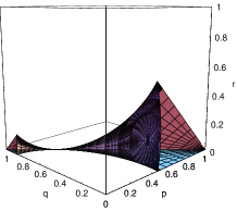
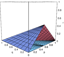
(a)(b)
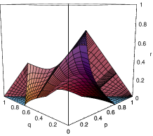
(c)(d)

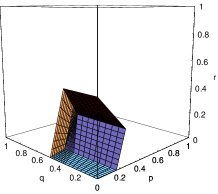
Figure 1: Comparison of the regions of $4\otimes 4$ rotationally invariant states (57) (remember that $p+q+r\leq 1$) detected by three separability criteria lying behind the bounds (4), (13), and (53). Plot (a) is made for the entropic inequality (8) with $\alpha=2$, which corresponds to the bound (4) in the sense that the latter works iff the former detects entanglement. Plot (b) is made for the separability criterion $\mathrm{Tr}(\varrho\varrho^{\Gamma_{U}})\geq 0$ (with $U$ being $4\times 4$ antisymmetric matrix with only nonzero elements $\pm 1$ lying on its anti–diagonal) appearing in the bound (53). Finally, plot (c) shows region detected by the entanglement witness $\mathcal{W}_{\mathcal{V}}$ appearing in the bound (13). For completeness plot (d) presents the region of PPT $4\otimes 4$ rotationally invariant states.

In Fig. 2 one has quantitative comparison of bounds (4) and (53). As previously, for completeness we also studied the bound (13). It is clear that even though our bound is worse in the sense that it provides lower values, it works in the region in which the bound (4) does detect anything.

(a)     
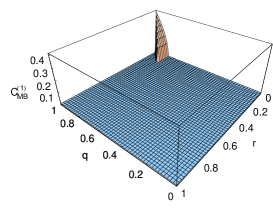
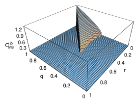
(b)     
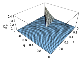
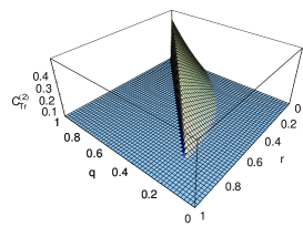
(c)

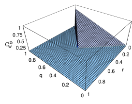
Figure 2: Quantitative comparison of three bounds, the bound (4) (plots (a)), our bound (53) (plots (b)), and the bound (13) (plot (c)) for the class of states (57) for different values of the parameters $p$, $q$, and $r$ ($C_{\mathrm{MB}}^{(i)}$, $C_{\mathrm{Tr}}^{(i)}$, and $C_{W}^{(2)}$ stand for the functions appearing on the right–hand sides of these bounds). Left plot is made for $p=0$, while the right one for $q=0$ (in the case of (13) only one bound is plotted for $q=0$ as the one for $p=0$ gives always zero). Though the new bound (53) provides lower values it detects entanglement in places where the MB bound as well as the bound (13) give zero.

V Measurable upper bounds on other concurrences

Here we discuss a possibility to generalize the upper bound (7) on $C$ provided in Ref. Guo . This bound follows straightforwardly from the concavity of the function $\sqrt{1-x^{2}}$. Here we point out that this reasoning may be immediately extended into the whole class of concurrences introduced firstly in Ref. Sinolecka and then considered, e.g., in Refs. Jap ; Gour . Further, we point out some possibilities of extending this bounds to a more general class of entanglement monotones. Moreover, we discuss these concurrences and obtained upper bounds in the context of the so–called Schmidt number of a density matrix Terhal , which is also an entanglement monotone.

Let us firstly introduce some notations. Let $\varrho$ be a given $d\times d$ density matrix and $\lambda(\varrho)$ denote a $d$–dimensional vector consisting of eigenvalues of $\varrho$ (hereafter denoted by $\lambda_{i}(\varrho)$). Then, let $\sigma_{k}(x_{0},\ldots,x_{d-1})$ denote the so–called $k$th elementary symmetric polynomial of $d$ arguments, that is

$$\sigma_{k}(x_{0},\ldots,x_{d-1})=\sum_{i_{1}<i_{2}<\ldots<i_{k}=0}^{d-1}x_{i_{1}}\ldots x_{i_{k}}.$$ (58)

Let us only mention that the first and last elementary symmetric polynomials, i.e., the ones corresponding to $k=1$ and $k=d$ are $x_{0}+\ldots+x_{d-1}$ and $x_{0}\cdot\ldots\cdot x_{d-1}$, respectively. Now, following Refs. Sinolecka ; Gour (with normalization adopted from Ref. Gour ) we can introduce the class of $d$ concurrences of the form

$$C_{k}(\varrho)=\inf_{\{p_{i},|\psi_{i}\rangle\}}\sum_{i}p_{i}C_{k}(|\psi_{i}\rangle)$$ (59)

with $C_{k}$ defined for pure states in the following way

$$C_{k}(|\psi\rangle)=h_{k}(\varrho_{r})\qquad(k=2,\ldots,d,\;r=A,B).$$ (60)

Here, like before, $\varrho_{r}$ stands for one of the reductions of $\varrho$ to a single–party state, while the functions $h_{k}$ are defined for $d\times d$ state $\rho$ as Gour :

$$h_{k}(\rho)=\left(\frac{\sigma_{k}(\lambda(\rho))}{\sigma_{k}(\lambda(\mathbbm{1}_{d}/d))}\right)^{1/k}.$$ (61)

First of all we need to emphasize that for purposes of the present section the concurrence $C$ is denoted by $C_{2}$, however, with different normalization. Namely, as it follows from Eqs. (60) and (61), now $C(|\psi\rangle)=\sqrt{[d/(d-1)](1-\mathrm{Tr}\varrho_{r}^{2})}$ and therefore it is normalized in such way that all the concurrences $C_{k}$ $(k=3,\ldots,d)$ give one for maximally entangled state $P_{+}^{(d)}$ irrespectively on $d$. For instance, the $d$th concurrence, also called $G$–concurrence Gour is given by $C_{d}(|\psi\rangle)\equiv G(|\psi\rangle)=d[\lambda_{0}(\rho_{r})\ldots\lambda_{d-1}(\rho_{r})]^{1/d}$.

Now we are prepared to proceed with our measurable upper bounds on $C_{k}$. For this purpose let us notice that, as shown in Ref. Gour , the functions $h_{k}$ are concave, i.e., they satisfy $h_{k}(p\rho_{1}+(1-p)\rho_{2})\geq ph_{k}(\rho_{1})+(1-p)h_{k}(\rho_{2})$ for any density matrices $\rho_{1}$ and $\rho_{2}$ and probability $0\leq p\leq 1$. Then, denoting by $\{p_{i},|\psi_{i}\rangle\}$ an optimal ensemble realizing $\varrho$ with respect to $C_{k}$, we are allowed to write

$$C_{k}(\varrho) = \sum_{i}p_{i}C_{k}(|\psi_{i}\rangle)$$ (62)

$$= \sum_{i}p_{i}h_{k}(\varrho_{r}^{(i)})$$

$$\leq h_{k}\left(\sum_{i}p_{i}\varrho_{r}^{(i)}\right)$$

$$= h_{k}(\varrho_{r})\qquad(r=A,B).$$

To get the first equality we utilized Eq. (60), while the inequality is a consequence of the aforementioned concavity of $h_{k}$. Moreover, $\varrho_{r}^{(i)}$ and $\varrho_{r}$ $(r=A,B)$ denote reductions to the $r$th subsystems of pure states $|\psi_{i}\rangle$ and $\varrho$, respectively.

Using explicit forms of $h_{f}$ (see (61)), the above bounds can be stated in the following form

$$\displaystyle C_{2}(\varrho)\leq\sqrt{\frac{d}{d-1}\left(1-\mathrm{Tr}\varrho_{r}^{2}\right)}$$

$$\displaystyle C_{3}(\varrho)\leq\sqrt[3]{\frac{d^{2}}{(d-1)(d-2)}\left(1-3\mathrm{Tr}\varrho_{r}^{3}+2\mathrm{Tr}\varrho_{r}^{2}\right)}$$

$$\vdots$$

$$\displaystyle C_{d}(\varrho)\leq d\left[\det(\varrho_{r})\right]^{1/d}.$$ (63)

In the first inequality one recognizes the bound (7) provided in Guo , however, with different normalization.

Let us notice that we can formalize the above considerations in a little bit more general way. Let $\mathcal{C}$ be a function defined for any pure state $|\psi\rangle\in\mathbbm{C}^{d}$ as $\mathcal{C}(|\psi\rangle)=h(\varrho_{A(B)})$ with $h$ denoting some polynomial function of eigenvalues of $\varrho_{A(B)}$ ($\varrho_{A(B)}$ denotes one of the subsystems of $\varrho$). On knows NielsenMajor that $\mathcal{C}$ can be an entanglement monotone for pure states if and only if $h$ is a Schur–concave function. That is, if it is a symmetric function obeying the following condition

$$\lambda(\sigma_{1})\succ\lambda(\sigma_{2})\quad\Rightarrow\quad h(\sigma_{1})\leq h(\sigma_{2})$$ (64)

for any $\sigma_{1}$ and $\sigma_{2}$. The expression $\lambda(\sigma_{1})\succ\lambda(\sigma_{2})$ means that eigenvalues of $\sigma_{1}$ majorize those of $\sigma_{2}$, i.e., the inequalities $\sum_{i=1}^{k}\lambda_{i}(\sigma_{1})\geq\sum_{i=1}^{k}\lambda_{i}(\sigma_{2})$ are satisfied for $k=1,\ldots,d-1$ and equality holds for $k=d$ (note that due to the fact that $\sigma_{1}$ and $\sigma_{2}$ are normalized this condition is satisfied naturally).

Extension of $\mathcal{C}$ to all mixed states can be done using the concept of convex roof. Now assuming that $h$ is a concave function and following the reasoning given in Eq. (62), one immediately have that $\mathcal{C}(\varrho)\leq h(\varrho_{A(B)})$. We know from Ref. Brun that any polynomial function of $\varrho_{A(B)}$ is measurable as a mean value of some quantum observable on some amount of copies of $\varrho_{A(B)}$ (the amount of copies depends on the degree of a measured polynomial). Concluding, we have a quite general statement saying that any such entanglement monotone can be upper bounded by some measurable function of a given state.

Finally, it is interesting to discuss this bounds in the context of another entanglement monotone, namely the Schmidt number Terhal . Let us recall that the Schmidt number of a bipartite mixed state $\varrho$ is defined as

$$SN(\varrho)=\min_{\{p_{i},|\psi_{i}\rangle\}}\max_{i}SR(|\psi_{i}\rangle),$$ (65)

with $SR(|\psi\rangle)$ being the so–called Schmidt rank of the pure state $|\psi\rangle$, i.e., the number of nonzero Schmidt coefficients in the Schmidt decomposition of $|\psi\rangle$. It is clear that the concurrences $C_{k}$ $(k=1,\ldots,d)$ are directly connected to the notion of Schmidt rank for pure states Gour . Namely, one sees from the definition of $C_{k}$ (Eqs. (60) and (61)) and the symmetric polynomials $\sigma_{k}$ (58) that the Schmidt rank of $|\psi\rangle$ is $l$ if and only if $C_{k}(|\psi\rangle)\neq 0$ for $k\leq l$ and $C_{k}(|\psi\rangle)=0$ for $k=l+1,\ldots,d$. This reasoning can also be extended to the case of mixed states. More precisely, we can prove that $SN(\varrho)=l$ iff $C_{k}(\varrho)\neq 0$ for $k\leq l$ and $C_{k}(\varrho)=0$ for $k=l+1,\ldots,d$. Notice that if for some $k$, $C_{k}(\varrho)=0$ then also $C_{l}(\varrho)=0$ for $l\geq k$. This is because if $C_{k}(\varrho)=0$ then there exists such ensemble $\mathcal{E}(\varrho)=\{p_{i},|\psi_{i}\rangle\}$ realizing $\varrho$ that $SR(|\psi_{i}\rangle)<k$ for each $i$. This, by virtue of what was said above, means that $C_{l}(|\psi_{i}\rangle)=0$ for any $l\geq k$ and therefore the ensemble $\mathcal{E}(\varrho)$ is also the optimal one for $C_{l}$ with $l\geq k$. For a similar reason if $C_{l}(\varrho)\neq 0$ then also $C_{k}(\varrho)\neq 0$ for $k\leq l$. Since $C_{l}(\varrho)$ all the ensembles realizing $\varrho$ have to contain at least one pure state with Schmidt rank greater or equal to $l$. Otherwise, $C_{l}$ would have to be zero. This causes that all the concurrences $C_{k}$ with $k\leq l$ have to be nonzero. Let us notice that the above two facts follow also from the inequality given in Gour , namely,

$$C_{2}^{2}(|\psi\rangle)\geq C_{3}^{3}(|\psi\rangle)\geq\ldots\geq C_{d}^{d}(|\psi\rangle).$$ (66)

By virtue of what was said it suffices to prove the statement that $SN(\varrho)=l$ iff $C_{l}(\varrho)\neq 0$ and $C_{l+1}(\varrho)=0$. For this purpose let us assume that $SN(\varrho)=l$. Then, according to the definition of the Schmidt number, one sees that there exists as ensemble $\widetilde{\mathcal{E}}(\varrho)=\{q_{i},|\varphi_{i}\rangle\}$ realizing $\varrho$ for which $\max_{i}SR(|\varphi_{i}\rangle)=l$. This means on the one hand that $C_{k}(|\varphi_{i}\rangle)=0$ for any $i$ and $k=l+1,\ldots,d$. Consequently $C_{k}(\varrho)=0$ for $k>l$ and the ensemble $\widetilde{\mathcal{E}}(\varrho)$ is the optimal one for these concurrences. On the other hand, according to the definition of the Schmidt number, all ensembles realizing $\varrho$ must contain at least one pure state of which the Schmidt rank is not less than $l$. This means that $C_{k}(\varrho)\neq 0$ for $k\leq l$.

To deal with the opposite direction we assume that $C_{l}(\varrho)\neq 0$ and $C_{l+1}(\varrho)\neq 0$. From the latter we infer that there must exist an ensemble of $\varrho$ in which all the pure states have the Schmidt rank at most $l$ and therefore, according to (65), $SN(\varrho)\leq l$. On the other hand, since $C_{l}(\varrho)\neq 0$ all the ensembles must contain at least one state of which the Schmidt rank is greater or equal to $l$. This means finally that $SN(\varrho)\geq l$ and together with the previous fact that $SN(\varrho)\leq l$ gives eventually $SN(\varrho)=l$.

The above discussion leads us to the conclusion that the bounds (62) can be also applied to bound the Schmidt number of a given $\varrho$. Namely, if $h_{l}(\varrho_{r})=0$ (notice that then obviously $h_{k}(\varrho_{r})=0$ for $k=l,\ldots,d$), then $C_{k}(\varrho)=0$ for any $k=l,\ldots,d$. This, by virtue of the above statement, means that $SN(\varrho)<l$. Therefore measuring upper bounds on the concurrences $C_{k}$ we can also get information about the Schmidt number of $\varrho$.

VI Conclusion

The general aim of the paper was to provide different ways of improving existing measurable bounds on entanglement measures. Measurable in the sense that the bounding functions can be written as a mean value of some quantum observable on a single or many copies of a state. Here we concentrated on those which can be measured collectively on two copies of a state. Though being rather harder to perform experimentally (one has to have several identical uncorrelated copies of given $\varrho$ at the same time) (see Ref. Enk2 ) such bounds in general work better (in the sense that they detect more states) than the ones based on linear witnesses.

In the first step we have provided another proof of the recent Mintert–Buchleitner bound MintertBuchleitner on concurrence and its multipartite generalization from Ref. Aolita . Then we have discussed possible improvements of this bounds which could follow from the proof. Though we were not able to provide a class of states for which the bound could be improved (and still be measurable) it seems that it is still interesting to investigate this approach.

Next, we have made an attempt to find other lower bounds on concurrence that could also be measured on copies of a given state. Firstly, relating the concurrence to the generalized robustness of entanglement and utilizing properties of the latter we have provided a way of bounding the former by mean values of entanglement witnesses obeying $W\leq\mathbbm{1}_{d}$. This, to some extent, can also be considered as a generalization of the result of Ref. BreuerBound (see Eq. 13). Then, choosing appropriately observables satisfying the above constraint we have obtained the whole class of bounds on concurrence depending on an arbitrary positive map and measurable on two copies of a state. Interestingly, using this approach one can also provide a different proof of the MB bound. More precisely, our method can be shown to reproduce the bound (4) when one considers the reduction map. In particular, we have investigated this bound for the transposition map on the class of $4\otimes 4$ rotationally invariant states and showed that, though rather less sharp, it works for regions for which the Mintert–Buchleitner bound gives zero.

Finally, we have provided a general reasoning leading to upper measurable bounds on the class of entanglement monotones. In particular, we have discussed these bounds for the class of concurrences provided in Refs. Sinolecka ; Gour .

Clearly, since as at least in the case of investigated states, the presented method works better than the MB bound, it is worth to be studied further. Namely, one has to try to optimize the utilized entanglement witnesses (through the constants $\alpha_{\rho}^{\Lambda}$) to improve the tightness of the bounds. This in general seems to be a rather hard task. In the case of the reduction map $R$ some steps towards optimization can be made using the bound on fidelity Miszczak , as it is pointed out in the paper. The procedure then leads to the MB result.

On the other hand, one could investigate other positive maps than the transposition one. For instance it would be particularly interesting to study also the indecomposable maps as it could give us measurable bounds detecting bound entangled states. This could lead to experimental detection of bound entanglement through joint measurements on two copies of a state. Finally, it would be desirable to derive similar measurable bounds using the recent entropic–like inequalities (RAJSPH ; RAJS ; RAJS2 ), which were shown to detect more entangled states than the entropic inequalities (8). Also, one could try to get similar bounds for the other concurrences as for instance $C_{k}$.

Finally, let us stress that all of the presented bounds concern mixed states, i.e., realistic situations in which the preparation of entangled states is affected by noise, or where an initially ideal entangled state undergoes dephasing. Experimental detection of these bounds can be realized using the set up of Ref. Schmid for photons, but generalization to atom or ion pairs are straightforward. Still, the presented bounds require preparation of two (or in general more) identical copies of the state of the system, and this process, is, of course, also subject to experimental imperfections. Fortunately, as in the case of Mintert–Buchleiner bound, all of our results are easily generalized for pairs of different states. As demonstrated in Ref. Schmid , this allows to obtain conclusive information about the entanglement of the state even in the worst case when the second copy is maximally entangled (i.e., gives the main contribution to the bound), provided the state of the system is entangled sufficiently strongly.

VII Acknowledgments

We are grateful to Daniel Cavalcanti, Otfried Gühne, Julia Stasińska, Julio de Vicente, and Karol Życzkowski for discussions. This work was prepared under the financial support from EU Programmes IP ”SCALA” and STREP ”NAMEQUAM”, Spanish MEC grants (FIS 2005-04627, FIS2008-00 and Consolider Ingenio 2010 ”QOIT”), and Humboldt Foundation.

References

- (1) R. Horodecki, P. Horodecki, M. Horodecki, and K. Horodecki, Rev. Mod. Phys. 81, 865 (2009).
- (2) P. Zoller et al., Eur. Phys. J. D 36, 203 (2005).
- (3) O. Gühne and G. Tóth, Phys. Rep. 474, 1 (2009).
- (4) A. G. White, J. R. Mitchell, O. Nairz, and P. G. Kwiat, Phys. Rev. A 58, 605 (1998).
- (5) H. Häffner, W. Hänsel, C. F. Roos, J. Benhelm, D. Chek–al–kar, M. Chwalla, T. Korber, U. D. Rapol, M. Riebe, P. O. Schmidt, C. Becher, O. Gühne, W. Dür, and R. Blatt, Nature 438, 643 (2005).
- (6) J. K. Korbicz, O. Gühne, M. Lewenstein, H. Häffner, C. F. Roos, and R. Blatt, Phys. Rev. A 74, 052319 (2006).
- (7) G. Jaeger, M. A. Horne, and A. Shimony, Phys. Rev. A 48, 1023 (1993); H. Weinfurter and Żukowski, Phys. Rev. A 64, 010102 (2001).
- (8) J. S. Bell, Speakable and Unspeakable in Quantum Mechamics, (Cambridge University Press, Cambridge, 2004); J. F. Clauser, M. A. Horne, A. Shimony, and R. A. Holt, Phys. Rev. Lett. 23, 880 (1969).
- (9) R. F. Werner, Phys. Rev. A 40, 4277 (1989).
- (10) J. Barrett Phys. Rev. A 65, 042302 (2002); G. Tóth and A. Acín, Phys. Rev. A 74, 030306 (2006); M. L. Almeida, S. Pironio, J. Barrett, G. Tóth, and A. Acín , Phys. Rev. Lett. 99, 040403 (2007).
- (11) R. F. Werner and M. Wolf, Quant. Inf. Comp. 1, 1 (2001).
- (12) M. Horodecki, P. Horodecki, and R. Horodecki, Phys. Lett. A 223, 1 (1996).
- (13) B. M. Terhal, Phys. Lett. A 271, 319 (2000).
- (14) O. Gühne, P. Hyllus, D. Bruss, A. Ekert, M. Lewenstein, C. Macchiavello, and A. Sanpera, Phys. Rev. A 66, 062305 (2002).
- (15) M. Barbieri, F. De Martini, G. Di Nepi, P. Mataloni, G. M. D’Ariano, and C. Macchiavello, Phys. Rev. Lett. 91, 227901 (2003).
- (16) M. Bourennane, M. Eibl, C. Kurtsiefer, S. Gaertner, H. Weinfurter, O. Gühne, P. Hyllus, D. Bruss, M. Lewenstein, and A. Sanpera, Phys. Rev. Lett. 92, 087902 (2004).
- (17) J. M. Sancho and S. F. Huelga, Phys. Rev. A 61, 042303 (2000); A. Acín, R. Tarrach and G. Vidal, Phys. Rev. A 61, 062307 (2000).
- (18) S. P. Walborn, P. H. Souto Ribeiro, L. Davidovich, F. Mintert, and A. Buchleitner, Nature 440, 1022 (2006).
- (19) P. Horodecki, Phys. Rev. Lett. 90, 167901 (2003).
- (20) F. Mintert and A. Buchleitner, Phys. Rev. Lett. 98, 140505 (2007).
- (21) R. Augusiak, M. Demianowicz, and P. Horodecki, Phys. Rev. A 77, 030301(R) (2008).
- (22) P. Horodecki, Phys. Rev. A 68, 052101 (2003).
- (23) P. Horodecki and A. Ekert, Phys. Rev. Lett. 89, 127902 (2002).
- (24) J. K. Korbicz et al., Phys. Rev. A 78, 062105 (2008).
- (25) O. Gühne and N. Lütkenhaus, Phys. Rev. Lett. 96, 170502 (2006).
- (26) O. Gühne, Phys. Rev. Lett. 92, 117903 (2004); G. Tóth, C. Knapp, O. Gühne, and H. J. Briegel, Phys. Rev. Lett. 99, 250405 (2007).
- (27) J. K. Korbicz, J. I. Cirac, and M. Lewenstein, Phys. Rev. Lett. 95, 120502 (2005); ibid. 95, 259901(E) (2005).
- (28) H. F. Hofmann and S. Takeuchi, Phys. Rev. A 68, 032103 (2003).
- (29) O. Gühne and M. Lewenstein, Phys. Rev. A 70, 022316 (2004).
- (30) J. I. de Vicente and J. Sánchez–Ruiz, Phys. Rev. A 71, 052325 (2005).
- (31) A. Acín, D. Bruss, M. Lewenstein, and A. Sanpera, Phys. Rev. Lett. 87, 040401 (2001).
- (32) O. Gühne, P. Hyllus, D. Bruss, A. Ekert, M. Lewenstein, C. Macchiavello, and A. Sanpera, J. Mod Opt. 50, 1079 (2003).
- (33) M. Horodecki, Quant. Inf. Comp. 1, 27 (2001).
- (34) S. Virmani and M. B. Plenio, Quant. Inf. Comp. 7, 1 (2007).
- (35) F. Mintert, Appl. Phys. B 89, 493 (2007).
- (36) H.–P. Breuer, J. Phys. A. 39, 11847 (2006).
- (37) F. Mintert, Phys. Rev. A 75, 052302 (2007).
- (38) L. Aolita, A. Buchleitner, and F. Mintert, Phys. Rev. A 78, 022308 (2008).
- (39) C.-J. Zhang et al., Phys. Rev. A 78, 042308 (2008).
- (40) F. Bovino et al., Phys. Rev. Lett. 95, 240407 (2005).
- (41) Ch. Schmid et al., Phys. Rev. Lett. 101, 260505 (2008).
- (42) C. Moura Alves, and D. Jaksch, Phys. Rev. Lett. 93, 110501 (2004).
- (43) S. J. van Enk, N. Lütkenhaus, and H. J. Kimble, Phys. Rev. A 75, 052318 (2007);
- (44) S. J. van Enk, Phys. Rev. Lett 102, 190503 (2009).
- (45) F. S. G. L. Brandão, Phys. Rev. A 72, 022310 (2005).
- (46) F. S. G. L. Brandão and R. O. Vianna, Int. J. Quant. Inf. 4, 331 (2006).
- (47) K. M. R. Audenaert and M. B. Plenio, New J. Phys. 8, 266 (2006).
- (48) O. Gühne, M. Reimpell, and R. F. Werner, Phys. Rev. Lett. 98, 110502 (2007).
- (49) O. Gühne, M. Reimpell, and R. F. Werner, Phys. Rev. A 77, 052317 (2008).
- (50) J. Eisert, F. G. S. L. Brandão, and K. M. R. Audenaert, New. J. Phys. 9, 46 (2007).
- (51) H. Wunderlich and M. B. Plenio, arXiv:0902.2093.
- (52) A. Uhlmann, Rep. Math. Phys. 9, 273 (1976).
- (53) R. Jozsa, J. Mod. Opt. 41, 2315 (1994).
- (54) J. A. Miszczak, Z. Puchała, P. Horodecki, A. Uhlmann, K. Życzkowski, Quant. Inf. Comp. 9, 103 (2009).
- (55) Z. Ma, D.–L. Deng, F.–L. Zhang, J.–L. Chen, Phys. Lett. A 373, 1616 (2009).
- (56) M. Sinołȩcka, M. Kuś, and K. Życzkowski, Acta Phys. Pol. B 33, 2081 (2002).
- (57) H. Fan, K. Matsumoto, and H. Imai, J. Phys. A 36, 4151 (2003).
- (58) G. Gour, Phys. Rev. A 71, 012318 (2005).
- (59) P. Rungta et al., Phys. Rev. A 64, 042315 (2001).
- (60) S. Hill and W. K. Wootters, Phys. Rev. Lett. 78, 5022 (1997).
- (61) A. R. R. Carvalho, F. Mintert, and A. Buchleitner, Phys. Rev. Lett. 93, 230501 (2004).
- (62) A. Borras, A. P. Majtey, A. R. Plastino, M. Casas, and A. Plastino, Phys. Rev. A 79, 022112 (2009).
- (63) R. Horodecki, P. Horodecki, and M. Horodecki, Phys. Lett. A 210, 377 (1996).
- (64) R. Horodecki and P. Horodecki, Phys. Lett. A 194, 147 (1994).
- (65) M. Horodecki and P. Horodecki, Phys. Rev. A 59, 4206 (1999).
- (66) B. M. Terhal, Theor. Comput. Sci. 287, 313 (2002).
- (67) K. G. H. Vollbrecht and M. M. Wolf, J. Math. Phys. 43, 4299 (2002).
- (68) S. Abe and A. K. Rajagopal, Physica A 289, 157 (2001).
- (69) C. Tsallis, S. Lloyd, and M. Baranger, Phys. Rev. A 63, 042104 (2001).
- (70) J. Batle, M. Casas, A. Plastino, and A. R. Plastino, Phys. Rev. A 71, 024301 (2005).
- (71) N. J. Cerf,C. Adami, R. M. Gingrich, Phys. Rev. A 60, 898 (1999).
- (72) R. Augusiak, J. Stasińska, and P. Horodecki, Phys. Rev. A 77, 012333 (2008).
- (73) R. Augusiak and J. Stasińska, Phys. Rev. A 77, 010303(R) (2008).
- (74) R. Augusiak and J. Stasińska, New J. Phys. 11, 053018 (2009).
- (75) K. Chen, S. Albeverio, and S.–M. Fei, Phys. Rev. Lett. 95, 040504 (2005).
- (76) A. Datta, S. T. Flammia, A. Shaji, and C. M. Caves, Phys. Rev. A 75, 062117 (2007).
- (77) J. I. de Vicente, Phys. Rev. A 75, 052320 (2007); Phys. Rev. A 77, 039903(E) (2008).
- (78) H.–P. Breuer, Phys. Rev. Lett. 97, 080501 (2006).
- (79) W. Hall, J. Phys. A 40, 6183 (2007).
- (80) S. Boyd and L. Vandenberghe, Convex Optimization, Cambridge University Press, Cambridge, 2004.
- (81) K. M. R. Audenaert and S. L. Braunstein, Commun. Math. Phys. 246, 443 (2004).
- (82) P. Rungta and C. M. Caves, Phys. Rev. A 67, 012307 (2003).
- (83) A. Uhlmann, J. Phys. A 34, 7047 (2001).
- (84) M. Hellmund and A. Uhlmann, Phys. Rev. A 79, 052319 (2009).
- (85) R. Hildebrand, J. Math. Phys. 48, 102108 (2007).
- (86) J. Dodd and M. A. Nielsen, Phys. Rev. A 66, 044301 (2002).
- (87) M. Steiner, Phys. Rev. A 67, 054305 (2003).
- (88) G. Vidal and R. Tarrach, Phys. Rev. A 59, 141 (1999).
- (89) M.–D. Choi, Linear Algebra Appl. 10, 285 (1975).
- (90) A. Jamiołkowski, Rep. Math. Phys. 3, 275 (1972).
- (91) I. Bengtsson, K. Życzkowski, Geometry of Quantum States, Cambridge Univ. Press, Cambridge, 2006.
- (92) R. F. Werner and A. S. Holevo, J. Math. Phys. 43, 4353 (2002).
- (93) B. M. Terhal and P. Horodecki, Phys. Rev. A 61, 040301 (2000).
- (94) M. A. Nielsen, Phys. Rev. Lett. 83, 436 (1999).
- (95) T. A. Brun, Quant. Inf. Comp. 4, 401 (2004).
- (96) C. J. Isham, N. Linden, and S. Scheckenberg, J. Math. Phys. 35, 6360 (1994).