Multiple Hypothesis Testing in Pattern Discovery

Abstract

The problem of multiple hypothesis testing arises when there are more than one hypothesis to be tested simultaneously for statistical significance. This is a very common situation in many data mining applications. For instance, assessing simultaneously the significance of all frequent itemsets of a single dataset entails a host of hypothesis, one for each itemset. A multiple hypothesis testing method is needed to control the number of false positives (Type I error). Our contribution in this paper is to extend the multiple hypothesis framework to be used with a generic data mining algorithm. We provide a method that provably controls the family-wise error rate (FWER, the probability of at least one false positive) in the strong sense. We evaluate the performance of our solution on both real and generated data. The results show that our method controls the FWER while maintaining the power of the test.

Keywords: Multiple hypothesis testing, Pattern mining, Frequent itemsets

1 Introduction

This paper addresses the problem of assessing the statistical significance of the patterns produced by data mining algorithms. In traditional statistics the issue of significance testing has been thoroughly studied for many years. Given observed data and a structural measure (namely, test statistic) calculated from the data, a hypothesis testing method can be used to decide whether the observed data was drawn from a given null hypothesis. Under this framework, randomization approaches help in producing multiple random datasets sampled from a specified null hypothesis. If the test statistic of the original data deviates significantly from the test statistics of the random datasets, then the null hypothesis can be discarded and the result can be considered significant.

Recently, there has been an increasing interest in randomization techniques for data mining (e.g. [5, 15]). For example, [5] introduced a method to sample 0–1 matrices uniformly at random such that the row and column margins of a matrix are preserved. The method is extended by [15] for real-valued matrices. As in the traditional framework from statistics, the randomized samples can be interpreted to be drawn from a null distribution and they are used to test the statistical significance of discovered patterns. In the case of 0–1 matrices, for example, the $p$-value of a frequent set could be defined as the fraction of randomized datasets that have a higher frequency for the set than with the original data.

The statistical significance testing problem is well understood when the hypothesis to be tested are known in advance and the number of hypothesis is fixed (see [4, 11, 19]). In the simplest case, there is only one hypothesis (such as a frequency of a given frequent set) and the statistical hypothesis test controls the probability of false positives, also called Type I error. A proper statistical significance test of level $\alpha$ (typical choices being $\alpha\in\{0.01,0.05\}$) falsely declares a pattern that follows the null distribution as significant (false positive) with a probability of at most $\alpha$.

The problem of multiple hypothesis testing arises when there are more than one hypothesis to test simultaneously. This is a very common situation in data mining: for instance, an algorithm for frequent set mining typically outputs a collection of itemsets whose frequency is above a user-specified threshold in the data. As a simple example, assume that we have 1000 independent patterns that all follow the null hypothesis (are random effects in the data). A naively applied statistical significance test of level $\alpha=0.05$ is likely to falsely declare about 50 of these 1000 patterns as significant, even though all of the measurements obey the null distribution. To remedy the independent evaluation of hypothesis, the theory of multiple hypothesis testing assesses a multiple comparison problem, that is, considers simultaneously a family of statistical inferences.

There exists traditional methods in statistics to tackle the problem of multiple hypothesis testing, of which the Bonferroni correction is the simplest and probably the best known. These methods vary with respect to the power, type of error they control and the assumptions they make of the dependency structure within the data. A common property for all of these methods is that as the number of hypothesis to be tested increases, the methods lose power, that is, they are less likely to find the hypothesis that are not from the null distribution.

A data mining algorithm can produce a host of patterns. For example, in the frequent set mining, the number of possible frequent sets is exponential in the number of attributes. If each pattern is considered as a separate hypothesis, then a direct application of multiple hypothesis testing would be too naive: the method would not declare any pattern as significant due to the large number of patterns to be tested.

A possible solution to overcome this problem consists of limiting the hypothesis space. For example, in frequent set mining one could only consider frequent sets of at most the given length. Another limiting approach was proposed by [17] for the specific application of association rule mining, where the data is first split into two folds. The first half of the data is used to run the data mining algorithm to define the hypothesis (association rules), and the second half of the data is then used to test for the significance of those patterns using some of the known multiple hypothesis testing methods. Such an approach works when the data can be split into two halves that are independent one of the other, and also, when the algorithm can be run on partial data. However, these conditions are not feasible for all applications: consider for example finding patterns such as frequent subgraphs from a network, which cannot be trivially split into two independent components.

A completely different approach for multiple hypothesis testing in association rule mining was proposed by [9]. Their idea is to use bootstrap to find an upper bound for the deviation of the test statistic between random and original data, such that it controls the probability of falsely declaring a pattern significant. All association rules mined from the original data that have a larger test statistic deviation from its mean than the chosen threshold, will be declared significant. This method has the same limitations as [17] in that it can only be used for association rule mining. Furthermore, bootstrapping transactions does not break the dependency between antecedent and consequent. This is of course a choice of a null hypothesis, but it may not make sense in all association rule mining contexts.

Our contribution in this paper is to provide a proper definition of $p$-value for patterns using the randomized samples, and show that with this $p$-value the known multiple hypothesis testing methods can be used directly on the patterns output by a generic data mining algorithm, regardless of the potentially large number of possible patterns. We make no assumption on the data. The main contributions of this paper are: the definition of a $p$-value suitable for data mining applications; a general method to assess significant patterns using a valid statistical testing methodology; and experimental verification of the validity and power of the presented method.

The paper is organized as follows. In Section 2 we provide the problem statement and essential definitions and in Section 3 we state our contribution without any formal proof. In Section, 4 we give a summary of multiple hypothesis testing and prove the validity of our method; this section can be skipped in the first reading. Section 5 reviews the related methods, Section 6 contains experiments and the paper ends with the discussion in Section 7.

2 Formal problem statement

We consider the general case where we have a data mining algorithm $A$ that, given an input dataset $D$, outputs a set of patterns $P$, or $A(D)=P$. The set $P$ is a subset of a universe of all patterns ${\cal\mathcal{P}}$. For different input datasets, the algorithm may output a different set of patterns, still from ${\mathcal{P}}$. We further assume defined a test statistic $f(x,D)\in{\mathbb{R}}$, associated to an input pattern $x\in{\cal P}$ for the dataset $D$; large values of the statistic are assumed to be more interesting for the user. We assume that we have at our disposal a randomization algorithm with which one can sample $n$ datasets i.i.d. from the null distribution $\Pi_{0}$ corresponding to the null hypothesis $H_{0}$. Our intuition is that if the test statistic for a given pattern $x$ is an extreme value in the null distribution, then we can declare the pattern significant. We denote the datasets sampled from the null distribution by $D_{i}$, where $i\in[n]$, and $[n]=\{1,\ldots,n\}$.

Using the above definitions, we can define our problem as follows.

Problem 1

Given a data mining algorithm $A$, a dataset $D$, a test statistic $f$ and a null distribution $\Pi_{0}$, which of the patterns output by $A(D)$ are statistically significant?

In this work we apply our method to frequent itemset mining and association rule mining from 0–1 data, and also, frequent subgraph mining from networks. However, our formulation is general and, unlike much of the previous work, we do not restrict ourselves to any particular types of data nor patterns.

Example 1

In frequent itemset mining the dataset $D$ could be a 0–1 data matrix, the set of all possible patterns $\mathcal{P}$ could be all subsets of attributes (itemsets), the algorithm $A$ could be a level-wise algorithm with a given frequency threshold and the test statistic $f(x,D)$ could be the frequency of the itemset $x$ in data matrix $D$. The null distribution $\Pi_{0}$ could be the uniform distribution over all binary matrices of the same size with fixed row and column margins; datasets from this null distribution can be sampled using the swap randomization presented in [5]. Our objective would be to decide which of the frequent itemsets output by the algorithm $A$ are statistically significant.

The methods of statistical significance testing often make assumptions about the shape of the null distribution (e.g., that the statistics follow a normal distribution). We do not make such assumptions, but we require that the algorithm $A$ satisfies the minP-property, which will be defined later in Section 4.2.

3 Main contribution: A significance testing method

In this section we state succinctly the main contribution of this paper, that is, a method to test the significance of patterns within the framework discussed in Section 2. The detailed discussion with derivations and references are presented in Section 4, and the experimental results are presented in Section 6.

We first define two empirical $p$-values: the first one is the sample-based empirical $p$-value in Definition 2, which weights each randomized dataset equally; the second is the pool-based $p$-value in Definition 3, where the patterns obtained from the randomized datasets are weighted equally.

Definition 1 (Sample based empirical p-value)

Let $D$ be our original dataset, $D_{i}$ for $i\leq n$ be the $n$ datasets sampled from the null distribution and $D_{n+1}=D$. Let also $f(x,D)$ be the test statistic associated to an input pattern $x\in\mathcal{P}$ returned by algorithm $A$. We define the sample-based $p$-value as follows:

$$p_{D}^{sample}(x)=\frac{\sum_{i=1}^{n+1}h(x,D,D_{i})}{n+1},$$ (1)

where,

$$h(x,D,D^{\prime})=\left\{\begin{array}[]{lcl}\frac{\left|\{x^{\prime}\in A(D^{\prime})\mid f(x,D)\leq f(x^{\prime},D^{\prime})\}\right|}{\left|A(D^{\prime})\right|}&,&|A(D^{\prime})|>0\\ 0&,&|A(D)^{\prime}|=0\end{array}\right..$$ (2)

Definition 2 (Pool based empirical p-value)

Let $D$ be our original dataset, $D_{i}$ for $i\leq n$ be the $n$ datasets sampled from the null distribution and $D_{n+1}=D$. Let also $f(x,D)$ be the test statistic associated to an input pattern $x\in\mathcal{P}$ returned by algorithm $A$. We define the pool-based $p$-value as follows:

$$p_{D}^{pool}(x)=\frac{\sum_{i=1}^{n+1}|\{y\in A(D_{i})|f(y,D_{i})\geq f(x,D)\}|}{\sum_{i=1}^{n+1}|A(D_{i})|}.$$ (3)

The $p$-values of the sample-based method represent the probability that, given a random dataset from the null distribution of datasets, a test statistic has a more extreme value. The difference between the two methods becomes from the weight to patterns. In the pool-based method, each pattern of the output of any dataset is weighted equally. Therefore, the datasets that result in more patterns have more control over the $p$-value calculation. Conversely, the sample-based method treats each dataset equally and the patterns in a single dataset share the weight of the dataset uniformly.

Briefly, we denote by $p_{i},$ $i\in[m]$, where $[m]=\{1,\ldots,m\}$, and $m=|A(D)|$, the sorted empirical $p$-values for the patterns $A(D)$ given by Equation (1) or (3), i.e., $p_{1}\leq\dots\leq p_{m}.$ We

The family-wise error rate (FWER) is defined as the probability of falsely declaring at least one patten in $A(D)$ as significant, where $A(D)$ represents the set of patterns output by algorithm $A$ using dataset $D$. A more formal definition will be provided in the next section. To control the FWER at the level $\alpha$, we can apply the Holm-Bonferroni method [7], to obtain the so-called adjusted $p$-values. The equation to compute the adjusted $p$-value of a pattern $x_{i}$ under Holm-Bonferroni method is,

$$\tilde{p}_{i}^{H}=\left\{\begin{array}[]{lcr}\min(1,mp_{1})&,&i=1\\ \min\left(1,\max(\tilde{p}_{i-1}^{H},(m-i+1)p_{i})\right)&,&i>1\end{array}\right..$$ (4)

Then, we declare the pattern $x$ significant if its adjusted $p$-value satisfies $\tilde{p}_{i}^{H}\leq\alpha$. Note that the Holm-Bonferroni method is general and can be used with any definition of $p$-value when the number of hypothesis is fixed.

From here, our main result reads as follows.

Theorem 1

Given that the minP-property holds, we can declare the pattern $x_{i}$ significant (reject the null hypothesis) if the adjusted $p$-value satisfies $\tilde{p}_{i}^{H}\leq\alpha$ with the guarantee that the FWER is controlled at the level $\alpha$.

The proof of Theorem 1 is given later in Section 4.3. The proper definition of minP-property and a test for checking whether the calculated $p$-values on the data satisfy this property will be discussed before in Section 4.2. In practice, we will show in the experiments that in many practical cases this minP-property is satisfied.

4 Theory of multiple testing of data mining results

This section validates the result presented in Theorem 1. First, we provide the preliminaries for the multiple hypothesis testing framework; and next discuss the two empirical $p$-value calculation methods and the minP-property. Finally, we show the correctness of the main result of this paper.

In the remainder of the paper we ignore the sampling error due to the finite number of samples from the null distribution, that is, we assume that $n$ is large enough. We also assume that the data mining algorithm always outputs at least one pattern.

4.1 Multiple hypothesis testing

In this section we provide a short summary of the theory and methods of multiple hypothesis testing. See [4, 19] for a review and further references.

Consider the problem of testing simultaneously $m$ null hypothesis $H_{0i}$, $i\in[m]$. It is assumed that the number of hypothesis to be tested, $m$, is known in advance, while the numbers $m_{0}$ and $m_{1}=m-m_{0}$ of true and false null hypothesis, respectively, are unknown parameters. With each hypothesis we have associated a test statistic value $T_{i}$ and a corresponding $p$-value $p_{i}$, $i\in[m]$. A $p$-value $p_{i}$ is defined as a probability that the test statistic value is at least $T_{i}$ under the null hypothesis $H_{0i}$. The values of $p_{i}$s are sometimes called unadjusted $p$-values.

In the simplest case, there is only one hypothesis ($m=1$). A valid level $\alpha$ statistical test is such that the hypothesis is declared significant, i.e., the null hypothesis is rejected, if $p_{1}\leq\alpha$. This happens with a probability of at most $\alpha$ if the data is sampled from the null distribution. Falsely declaring a pattern significant (false positive) is called a Type I error, while falsely declaring a pattern non-significant (false negative) is called a Type II error. A standard approach is to specify an acceptable level $\alpha$ for the Type I error rate and construct a test, i.e., choose a test statistic, that minimizes the Type II error rate, that is, maximizes the power of the test.

For multiple hypothesis testing $m>1$, the situation is no longer as straightforward. Following [4], we denote by $R$ the number of hypothesis declared significant; by $S$ and $U$ the numbers of hypothesis correctly declared significant and non-significant, respectively; and by $V$ and $T$ the number of hypothesis declared incorrectly significant and non-significant, respectively. The count $V$ corresponds to the number of Type I errors (false positives), while $T$ corresponds to the number of Type II errors (false negatives). See Table 1 for a summary.

	Not declared	Declared
	significant	significant
True null hypothesis	$U$	$V$	$m_{0}$
Non-true null hypothesis	$T$	$S$	$m_{1}$
	$m-R$	$R$	$m$

Table 1: Multiple hypothesis testing. $R$ and $m$ are observed counts, while $S$, $T$, $U$, $V$, $m_{0}$ and $m_{1}$ are unknown. $V$ is the number of Type I errors and $T$ the number of Type II errors.

There are many ways to define the acceptable Type I error rate. We use the family-wise error rate (FWER). A statistical test that controls the FWER at level $\alpha$ is such that the probability of even one Type I error is at most $\alpha$, that is, $Pr(V>0)\leq\alpha$. Another control of Type I error is given by the false discovery rate (FDR), introduced by [2]. A statistical test that controls the FDR at level $\alpha$ is such that the expected fraction of Type I errors among the rejected hypothesis is at most $\alpha$, that is, $E(Q)\leq\alpha$, where $Q=V/R$ if $R>0$ and $0$ if $R=0$.

The choice of control depends on the application. If even one false positive would be disastrous, for example, the hypothesis would be about if the various drugs are safe to use, then it is appropriate to choose FWER. However, the FDR may be more appropriate choice, for example, if the objective is to identify hypothesis for further study.

The multiple hypothesis testing methods are often defined in terms of adjusted $p$-values. In the following, we review two tests — Bonferroni and Holm-Bonferroni — that can be used to compute the adjusted $p$-values while controlling the FWER.

The simplest and probably the best known multiple testing method that controls the FWER is the Bonferroni test. The adjusted $p$-values are given by

$$\tilde{p}_{i}^{B}=\min{\left(1,mp_{i}\right)}.$$ (5)

A hypothesis $i\in[m]$ is declared significant if $\tilde{p}_{i}^{B}\leq\alpha$.

Advantages of the Bonferroni test are that it is simple and easy to understand and implement, and that an adjusted $p$-value of a hypothesis depends only on the unadjusted $p$-value of the same hypothesis.

We do not use the Bonferroni test, because a more powerful and slightly more complicated test that controls the FWER was introduced by [7]: the Holm-Bonferroni test given in Equation (4). Neither Bonferroni nor Holm-Bonferroni tests make any assumptions on the dependency structure of the hypothesis. In our application this is an important property, as the hypothesis (patterns output by the data mining algorithm) can have strong correlations.

In the presence of $n$ samples from the null distribution we can use empirical $p$-values, see [14] for discussion.

4.2 The minP-property assumption

Before showing the validity of our method, we present first the minP-property that we require the algorithm to satisfy. This property guarantees weak control over the FWER with the absence of false null hypotheses, i.e., under the complete null hypothesis.

Definition 3 (minP-property)

Assume a dataset $D^{\prime}$ is sampled from the null distribution $\Pi_{0}$. Then it holds $\forall t\in[0,1]$ that

$$Pr(|A(D^{\prime})|\min_{x\in A(D^{\prime})}p_{D^{\prime}}(x)\leq t|H_{0}^{C})\leq t,$$

where $p_{D^{\prime}}(x)$ is the empirical $p$-value of the pattern $x$ output by the algorithm with dataset $D^{\prime}$, and $H_{0}^{C}$ signifies the complete null hypothesis.

Indeed, the minP-property enforces constraint to the way the test statistics can vary for different number of outputs. If larger test statistics are encountered only for a small number of output patterns, there is an elevated risk of false positives. If a pattern has an extreme test statistic value, it will have a small $p$-value. For a small number of patterns, the Holm-Bonferroni adjustment will be small. If both cases are true, the adjusted $p$-value will also be small, possibly causing a false positive.

As shown later in Lemma 1, the minP property is always satisfied if the data mining algorithm always outputs a constant number of patterns. Our defined empirical $p$-values might not satisfy the minP-property in all cases when the number of patterns output by the algorithm varies. We define the following to test if the property holds.

Definition 4 (minP-test)

Let $\hat{p}_{i}=|A(D_{i})|\min_{x\in A(D_{i})}p_{D_{i}}(x)$. The minP-property is satisfied if for all $t\in[0,1]$,

$$\frac{|\{i|\hat{p}_{i}\leq t\}|}{n}\leq t.$$

Notice that the minP-test can be carried out visually by plotting $\frac{|\{i|\hat{p}_{i}\leq t\}|}{n}$ against $t$ and checking if the plotted line never exceeds the diagonal line.

Actually, our two defined $p$-values admit the minP-property in a variety of situations. We make the following observation concerning both methods.

Lemma 1

The minP-property is always satisfied for both the sample and pool-based methods if the data mining algorithm $A$ outputs a constant number of patterns, that is, $m=|A(D^{\prime})|$ for any $D^{\prime}$. In this case, the two $p$-values behave in the same way.

For proving Lemma 1 we need first the following property.

Proposition 1

For real valued $y$ and $x$, that are distributed identically, and for any $\alpha\in[0,1]$, $Pr(Pr(x\leq y)\leq\alpha)=\alpha.$

• of Lemma 1. The sample-based $p$-values can be written as:

  $$p_{D^{\prime}}^{sample}(x) = \frac{\sum_{i=1}^{n+1}h(x,D^{\prime},D_{i})}{n+1}$$

  $$\stackrel{{\scriptstyle n\rightarrow\infty}}{{\longrightarrow}} \sum_{\hat{D}}Pr(\hat{D})h(x,D^{\prime},\hat{D}).$$

  With this, the minP-property is then

  $$Pr(m\min_{x\in A(D^{\prime})}p_{D^{\prime}}^{sample}(x)\leq\alpha|H_{0}^{C})$$

  $$= \sum_{D^{\prime}}Pr(D^{\prime})\mathbb{I}\left(m\min_{x\in A(D^{\prime})}p_{D^{\prime}}^{sample}(x)\leq\alpha\right)$$

  $$= \sum_{D^{\prime}}Pr(D^{\prime})\mathbb{I}\left(\min_{x\in A(D^{\prime})}\left(\sum_{\hat{D}}Pr(\hat{D})\left|\{y\in A(\hat{D})\mid f(x,D^{\prime})\leq f(y,\hat{D})\}\right|\right)\leq\alpha\right)$$

  $$\leq \sum_{D^{\prime}}Pr(D^{\prime})\mathbb{I}\left(\sum_{\hat{D}}Pr(\hat{D})\mathbb{I}\left(\max_{x\in A(D^{\prime})}f(x,D^{\prime})\leq\max_{y\in A(\hat{D})}f(y,\hat{D})\right)\leq\alpha\right)$$

  $$= \alpha.$$

  The function $\mathbb{I}(\cdot)$ returns 1 if the condition is true and 0 otherwise. The last step follows from Proposition 1. To prove the equality of the methods, consider

  $$p_{D^{\prime}}^{sample}(x) = \frac{\sum_{i=1}^{n+1}h(x,D^{\prime},D_{i})}{n+1}$$

  $$= \frac{1}{(n+1)m}\sum_{i=1}^{n+1}|\{y\in A(D_{i})|f(y,D_{i})\geq f(x,D^{\prime})\}|$$

  $$= p_{D^{\prime}}^{pool}(x).$$

  $\Box$

That is, in the simplest case, where the data mining algorithm is expected to output approximately constant number of patterns, the minP-property is expected to hold to a good accuracy.

The minP-property is in practice not too restrictive, as shown later by our experiments. A data mining algorithm may violate the property if the distribution of $p$-values depends strongly on the number of patterns output by the algorithm.

Example 2

Adversarial example. Assume that we have a data mining algorithm $A$ and null distribution such that when a dataset $D$ is sampled from the null distribution the following is satisfied. With probability of $\frac{4}{5}$, the algorithm $A(D)$ outputs one pattern with a sample-based $p$-value $p_{D}^{sample}(x)$ sampled from uniform $U(\frac{1}{10},1)$; and with probability of $\frac{1}{5}$, the algorithm $A(D)$ outputs two patterns, one having a $p$-value from $U(0,\frac{1}{10})$ and another having a $p$-value from $U(\frac{1}{10},1)$. Here $U(a,b)$ is a probability distribution over real numbers that is uniform over interval $[a,b]$ and zero elsewhere.

The above described pattern of $p$-values would occur for example if the algorithm would output with probability $\frac{4}{5}$ a pattern with a test statistics $f$ from $U(-1,0)$; and with probability of $\frac{1}{5}$ two patterns with test statistics from $U(-1,0)$ and $U(0,1)$, respectively.

Choose $t=\frac{3}{5}$ and denote $p^{\prime}=\min_{x\in A(D^{\prime})}p_{D^{\prime}}^{sample}(x)$. If the algorithm outputs one pattern ($m_{0}=1$) we have $Pr(m_{0}p^{\prime}\leq\frac{3}{5})=\frac{5}{9}$ — this happens with a probability of $\frac{4}{5}$. On the other hand, if the algorithm outputs two patterns ($m_{0}=2$) we have $Pr(m_{0}p^{\prime}\leq\frac{3}{5})=1$ (as the smallest $p$-value is always at most $\frac{1}{10}$).

Summarizing, $Pr(m_{0}p^{\prime}\leq\frac{3}{5})=\frac{4}{5}\times\frac{5}{9}+\frac{1}{5}\times 1=\frac{29}{45}\approx 0.644$, which does not satisfy the minP-property. Furthermore, the minP-property neither holds for the pool-based $p$-values in this example.

Assessing the minP-property under the combination of randomization method, algorithm and test statistic may be prohibitively complex to do analytically. Still Definition 4 corresponds to a test for the minP-property, which indicates whether the minP-property is violated.

In Figure 1, the visual test for minP-property is illustrated. The plot shows the empirical FWER under the complete null hypothesis for different acceptance levels for FWER. If the diagonal line is exceeded, the minP-property does not hold. However, since the method is approximate, slight violations may be due to sampling error and may be ignored.

Figure 1: Visual minP-test. The horizontal and vertical axes represent the acceptable and true FWER levels, respectively. The solid line represents the measured FWER for different acceptable FWER levels, and the dash dotted line represents the threshold that should not be exceeded. We have used association rule mining for all methods with Paleo dataset, see Section 6.2. Both methods coincide.

4.3 Validity of our method

We prove that our method defined in Theorem 1, is a valid level $\alpha$ test by an argument similar to the closed testing procedure [12] with minP test, which is arguably the most concise way to derive the Holm-Bonferroni test in the traditional multiple testing scenario. We finally conclude with the proof of Theorem 1.

• of Theorem 1. Assume that the data mining algorithm outputs $m$ patterns $A(D)=P_{0}\cup P_{1}$ such that the patterns in $P_{0}$ obey the null hypothesis and the patterns in $P_{1}$ do not, with $P_{0}\cap P_{1}=\emptyset$. Let $m_{0}=|P_{0}|$. If $m_{0}=0$ the FWER is always trivially controlled; in the following we consider the case $m_{0}>0$. Denote by $x^{\prime}$ the pattern in $P_{0}$ that has the smallest $p$-value, that is, $x^{\prime}=\arg{\min_{x\in P_{0}}{p_{D}(x)}}$. In the Holm-Bonferroni test of Equation (4), we violate the FWER ($V>0$) if and only if we declare $x^{\prime}$ significant. Let $m^{\prime}$ be the number of patterns with a $p$-value no smaller than $p_{D}(x^{\prime})$; $m^{\prime}$ obviously satisfies $m_{0}\leq m^{\prime}$. In the Holm-Bonferroni test we declare $x^{\prime}$ significant if $m^{\prime}p_{D}(x^{\prime})\leq\alpha$. Due to minP-property,

  $$Pr\{m^{\prime}p_{D}(x^{\prime})\leq\alpha\}\leq Pr\left\{m_{0}p_{D}(x^{\prime})\leq\alpha\big{|}H_{0}^{C}\right\}\leq\alpha.$$

  The first inequality holds, since $m_{0}\leq m^{\prime}$ and $P_{1}$ do not effect $p_{D}(x^{\prime}).$ Therefore,

  $$Pr\{x^{\prime}{\rm\leavevmode\nobreak\ declared\leavevmode\nobreak\ significant}\}\leq\alpha,$$

  and in other words, $V>0$ with a probability of at most $\alpha$. $\Box$

5 Related work

In the following section, we review the existing methods from the literature related to the multiple hypothesis testing within the data mining framework. Notice that none of these methods is directly comparable to our contribution. The reason for this is that they control different error or only calculate it, use specific randomization to derive the significance, or are defined only for specific types of patterns.

5.1 Methods measuring Type I errors

In [20], Zhang et al. mine significant statistical quantitative rules (SQ rules). The difference to our methods is that they only calculate FDR, where we prove strong control for FWER. Also, they restrict their approach to a specific setting in binary data and consider only one class of null hypotheses. Our methods are not restricted to a special type of pattern and allow a very broad spectrum of null hypotheses.

In the method of Zhang et al., the dataset is splitted into two sets of attributes $X$ and $Y$. The antecedent, i.e. an itemset, of a SQ rule is defined as a subset of $X$. A statistic value is also attached to each rule, where the value is calculated from the transactions that contain the antecedent in $X$, but only using the attributes in $Y$. The significances are calculated by randomizing the dataset so that the dependence between antecedent and consequent is broken, and the statistic values are stored for each randomized dataset and rule. Finally, a confidence interval for a single rule is defined as the interval to which $(1-\alpha)$ statistic values fall. FDR is not shown to be statistically controlled, but it is calculated by using randomized datasets and checking how many rules are declared significant with a certain $\alpha$. The value of FDR is then obtained by taking the mean of the numbers and dividing it by the number of rules discovered from the original data.

In [13], Megiddo et al. mine association rules and, given a threshold $\alpha$ for the raw $p$-values, calculate the expected number of Type I errors. Conversely, our methods have strong control for FWER. Furthermore, they consider only association rules, and thus the method might not be as general as our methods.

In the method of Megiddo et al., they start by first mining frequent itemsets and then using them to find association rules that have a sufficiently large minimum confidence. The $p$-values are calculated for itemsets from a Gaussian distribution with the mean set to the minimum support value used to mine the itemsets, and the variance set to the variance of a binomial distribution with the probability $\mathrm{(minimum\ support)}/\mathrm{(nr\ transactions)}$. The authors also discuss the $p$-values for association rules, but unfortunately do not explicitly state how to calculate them. The multiple testing procedure is then to construct random datasets with the same expected column margins as the original dataset. The $p$-values for all patterns in a single dataset are sorted ascending, and the mean of the smallest $p$-values over all datasets is calculated as $V_{1}$, then the second smallest as $V_{2}$, and so forth for $V_{k}$. These values define thresholds for $\alpha$-values. For instance, if $V_{1}<\alpha\leq V_{2}$, then the expected number of Type I errors is at most two for the level $\alpha$.

5.2 Method that controls the probability of at most $V_{0}$ Type I errors

A generalization of FWER is to control the probability that the number of Type I errors exceeds a specified number, $V_{0}.$ In other words, assure that $Pr(V>V_{0})\leq\alpha.$ Standard FWER is controlled when $V_{0}=0.$

The method by Lallich et al. [10] is similar to ours in that it draws random samples of datasets and defines control over FWER (or similar) Type I error measure. The difference is that they define to use bootstrapping, and thus the method might not be as general as ours as the properties of the method may depend on bootstrapping. Furthermore, the correction for multiple hypothesis is calculated directly, which may require assumptions [19] and strong control is not proven, which we do.

In the method, they first find a set of association rules from the original data, and calculate some statistic for each rule. Then they sample random datasets by using bootstrap over the transactions with replacement. For each rule, the same statistics are calculated in the random dataset, and the difference in the statistic values between the original and random data are computed. The differences are sorted in decreasing order and stored as $\epsilon(k,i)$, where $i$ is the index of a random dataset and $k$ is the rank of a difference. Finally, for a certain desired number $V_{0}$, a value $\epsilon(\alpha)$ is calculated that satisfies

$$\frac{|\{i|\epsilon(V_{0},i)\geq\epsilon(\alpha)\}|}{\mathrm{nr\ random\ datasets}}\leq\alpha.$$

The rules that have a statistic value higher than $\epsilon(\alpha)$ are selected.

5.3 Methods that control the FWER

In [1], Bay and Pazzani mine contrast sets. The similarly to our methods is the control of FWER, but they restrict themselves to contrast sets, where our methods are general. Furthermore, using Bonferroni correction may not be reasonable, since it is often overly conservative and provides no theoretical improvement over Holm-Bonferroni.

Contrast sets are similar to association rules but differ in that a good rule shows contrast between two groups of transactions. The data can be multivariate, but it is required that the transactions are grouped to disjoint sets. The $p$-values are calculated for contrast sets from a respective contingency table using $\chi^{2}$ approximation. The rules that have too small values in the contingency table for the $\chi^{2}$ to produce an adequate approximation are pruned away. Using the Bonferroni inequality, the authors define confidence thresholds for each size of itemset mined, which is dependent upon the number of candidates of a specific size generated when mining frequent itemsets,

$$\alpha_{l}=\min(\frac{\alpha}{2^{l}|C_{l}|},\alpha_{l-1}),$$

where $l$ is the level, or size of itemsets, and $|C_{l}|$ is the size of the candidate set for level $l$.

In [17, 18], Webb considers association rules and defines a method to overcome the problems caused by thresholding, with, for example, minimum support. The number of actual hypotheses may not correspond to the number of output patterns. Webb’s main contribution, the holdout method, is similar to our methods in that it considers the problematic scenario of varying number of outputs. The Holm-Bonferroni correction can be and is used in the paper, as do we. However, the method by Webb is limited to scenarios where the data can be split into two independent parts, and there is enough data to split it. Only association rules are considered in the paper. Splitting may not be possible for example with network data or spatial data. Furthermore, the data mining algorithm needs to be able to operate on partial data. Our methods do not have such constraints.

In the paper, Webb presents two methods by using the contingency table of an association rule to find out its $p$-value. The first method is to use normal Bonferroni-adjustment for the original $p$-values, where the multiplier is the number of all possible patterns of at most a preset maximum length set by the user. The other method is the holdout method. The data is splitted in two, and a part of the data, called exploratory data, is used to find the set of itemsets to consider using normal association rule mining methods. After that, the second part of the data, called holdout data, is used to assess the statistical significance of the set of rules.

5.4 Standard methods for FWER

The standard methods for adjusting raw $p$-values to control FWER include, among others, Bonferroni, Holm-Bonferroni, and Sidak [4], as well as resampling based methods of [19]. A common property of all of these methods is that they assume that the set of hypothesis (in our case, set of all possible patterns) are defined beforehand and there is a raw $p$-value for each of the potential patterns. This poses the problems explained in the introduction.

6 Experiments

In this section we show the tests carried out to assess the quality of the proposed methods.

6.1 Synthetic data

The first experiment was with synthetic data of real numbers, with which the performance of the methods can be measured in a controlled environment. The synthetic data follows the multivariate Gaussian distribution

$$\Pi_{0}(x)=\mathcal{N}(x,\mu,C),$$

where $\mu$ is the mean vector and $C$ the covariance matrix. The generated real values correspond to the test statistic values $f$ used.

We began by using the methods under the complete null hypothesis and measuring the empirical probability of rejecting at least one hypothesis, or $Pr(V>0|H_{0}^{C})$. This corresponds to the minP-test.

The randomized datasets were generated by drawing a random vector of length $k=100$ from the normal distribution with zero mean $\mu=0$ and covariance matrix

$$(C_{0})_{ij}=\begin{cases}1&,i=j\\ \sigma&,i\neq j\end{cases}.$$

The values in a random vector constitute a dataset $D$, which is also of size $k$. The parameter $\sigma\in[-\frac{1}{k-1},1]$ controls the amount of covariance between the data points. If $\sigma<-\frac{1}{k-1},$ the covariance matrix is no longer positive semi-definite, and therefore, no longer a proper covariance matrix. We used $\sigma\in\{-0.0099,0,0.1,0.25,0.5,0.99\}.$

To simulate data mining methods, we used three different ad-hoc algorithms. These are ${\mathrm{ge}_{1}}$, $\max_{10}$, and $\mathrm{rnd}_{10}$. Assume now that we have a dataset $D$ of real numbers. The first algorithm, ${\mathrm{ge}_{1}}$, outputs the set of values that are greater or equal to 1 in $D$. The second algorithm, $\max_{10}$, outputs the 10 largest values in $D$. And the third algorithm, $\mathrm{rnd}_{10}$, selects 10 numbers from $D$ uniformly at random.

A single run starts by generating a dataset $D$ from the null distribution. This data is then mined for patterns $P$ with a selected algorithm, which results in a set of real values. These values are the test statistics values of the mined patterns. Then, we draw $n=10000$ datasets from $\Pi_{0}$, and calculate $p$-values for all $P$ using both methods. Finally, the minimum value of the adjusted $p$-values are stored, which is $\min(|P|\min_{y\in P}(p_{D}(y)),1),$ separate for both methods.

We performed these runs 10000 times for each combination of algorithm and magnitude of covariance. Figure 2 depicts the results: the solid lines correspond to different magnitudes of covariance and represent for each value of $\alpha$ the empirical probability of $P(V>0).$

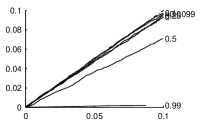
(a) ${\mathrm{ge}_{1}}$ with sample

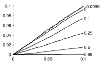
(b) ${\mathrm{ge}_{1}}$ with pool

(c) $\mathrm{rnd}_{10}$ with sample

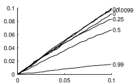
(d) $\mathrm{rnd}_{10}$ with pool

(e) $\max_{10}$ with sample

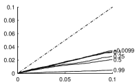
(f) $\max_{10}$ with pool

Figure 2: MinP-test results for synthetic data. The solid lines correspond to empirical probabilities of Type I error with a specific $\alpha$ level. To the right of line is the magnitude of covariance of the respective test. The dash-dotted line is the $Pr(V>0)=\alpha$ line, which should not be exceeded.

As shown in the figure, when the correlation is negative, $-0.0099$, and algorithm ${\mathrm{ge}_{1}}$ or $\mathrm{rnd}_{10}$ is used, $Pr(V>0)\approx\alpha$. This means that the proposed methods control the FWER very tightly in some cases. The important observation is that the controlled threshold is not exceeded, which translates to satisfying the minP-property.

The power was also tested with synthetic data of the same kind. Each dataset was constructed by randomizing samples from the multivariate Gaussian distribution with mean 0 for samples from the null distribution, and mean 4 for samples from the alternate distribution, and correlation between all samples. Hence,

$$(\mu)_{i}=\begin{cases}0&,i\leq m_{0}\\ 4&,m_{0}<i\leq m\end{cases},$$

and

$$(C_{0})_{ij}=\begin{cases}1&,i=j\\ \sigma&,i\neq j.\end{cases}$$

The number of null hypothesis was set to $m_{0}=80$. The same simulations with 10000 randomizations for datasets and 10000 overall runs, were performed for different correlations $\sigma\in\{-0.0099,0,0.1,0.25,0.5,0.99\}$ and the algorithm ${\mathrm{ge}_{1}}$. The probability of Type I error (FWER) and the mean fraction of Type II errors were calculated for both $p$-value calculation methods. Figure 3 depicts ROC-curves for $\sigma=0.5$ correlation with varying $\alpha.$

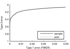
Figure 3: Power results for synthetic data. ROC-curve (varying $\alpha$) of the $p$-value calculation methods for $\sigma=0.5$ correlation.

To compare the methods for all correlations, we also calculated the area under curve (AUC) from the ROC-curves for both methods and all correlations. The results are shown in Figure 4.

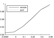
Figure 4: Power results for synthetic data. Area under curves of the ROC-curves for different $p$-value calculation methods and correlations. Higher value represents better accuracy.

As a conjecture from the synthetic data experiments, the minP-property was always satisfied and the power of both methods are very similar in these cases.

6.2 Association rules

The second experiment was a more practical data mining scenario, namely, association rule mining.

We used three different datasets: Paleo, Courses and Retail; all of which were used in [5]. The property values of these datasets are presented in Table 2.

Dataset	# of rows	# of cols	# of 1’s	density %
Paleo	124	139	1978	11.48
Courses	2405	5021	65152	0.54
Retail	88162	16470	908576	0.06

Table 2: Description of the datasets

Each dataset was randomized 1000 times by maintaining the column margins constant. Association rules were then mined from each dataset using the minimum support thresholds from [5]: $7$, $400$ and $200$ for $\textsc{Paleo},$ Courses and Retail, respectively. We used as test statistic $f$ the Fisher’s exact test between the antecedent and the consequent of an association rule. Holm-Bonferroni’s method was used to correct the $p$-values. Table 3 lists for different datasets the minimum support, number of rules in the original data, and the mean and standard deviation of the number of rules in the randomized datasets.

Dataset	minimum support	$|P|$	$|P_{i}|$
Paleo	7	9004	577.2(24.0)
Courses	400	51118	379.4(7.4)
Retail	200	4148	2703.9(16.1)

Table 3: Mining parameters and statistics for association rule mining. $|P|$ represents the number of association rules in the original data, and $|P_{i}|$ is the mean number of association rules with random data. Standard deviations are shown in parenthesis.

While randomizing, we carried out the minP-test for all combinations of dataset and $p$-value calculation method. The first half, 500, of randomizations were used to gather minimum $p$-values from the random datasets. By construction, the minimum $p$-values will necessarily correspond to the largest test statistic values, and therefore, for the first 500 random datasets, the largest test statistic value was stored from each. These were then calculated $p$-values using the latter 500 random datasets and both methods.

In all cases, the minP-property was clearly satisfied. Figure 1 depicts one test result; all other minP-test results are presented in Appendix A.1.

We also calculated the number of patterns found significant for different controlled FWER levels $\alpha$. These results are depicted in Figure 5. The results indicate, that sample is more powerful than pool in these cases. This is mostly due to the different $p$-value calculation methods, but can in part be because of the relative large number of patterns and limited number of randomizations.

For $\emph{sample},$ the results are intuitive: When $\alpha$ level, i.e., the accepted probability of making a Type I error, increases, the number of significant patterns increases. To conclude, the results are reasonable.

(a) Paleo

(b) Courses

(c) Retail

Figure 5: Association rule mining results for both $p$-value calculation methods and datasets. The lines depict the number of patterns found significant for different controlled FWER levels ($\alpha$).

6.3 Frequent itemsets

The third experiment is in similar context to the previous one. However, this time we mined for frequent itemsets.

The test statistic $f$ was a variant of the lift [17]:

$$f(x)=\frac{\mathrm{freq}(x)}{\prod_{A\in x}\mathrm{freq}(A)},$$ (6)

where $x$ is an itemset, $A$ is a single attribute, and $\mathrm{freq}(x)\in[0,1]$ is the relative frequency of itemset $x$. The same datasets were used as in association rule mining with the same minimum support thresholds. Additionally, we set the smallest frequent itemset size to 2, not to get individual columns as frequent itemsets. We used the same randomization method as above that preserves the column margins. We use the name Col for this method. The second randomization method we used was presented in [5] with the name swap randomization which additionally maintains the row margins. We will use the name Swap for this method. Note that we used exactly the same datasets, mining parameters and randomization methods as in [5].

Each dataset was randomized 10000 times with both methods. Table 4 lists for different datasets the minimum support, number of frequent itemsets in the original data, and the mean and standard deviation of the number of frequent itemsets in the randomized datasets. Note first that the expected numbers of frequent itemsets, and their standard deviations, are close to the numbers reported in [5]. The small differences are a result of different randomizations.

Dataset	minsup	$|P|$	$|P_{i}^{\mathrm{\textsc{Col}}}|$	$|P_{i}^{\mathrm{\textsc{Swap}}}|$
Paleo	7	2828	227.4(11.6)	266.9(14.8)
Courses	400	9678	146.6(2.8)	430.1(11.6)
Retail	200	1384	860.3(7.0)	1615.1(11.9)

Table 4: Mining parameters and statistics for frequent itemset maining. $|P|$ is the number of frequent itemsets with the original data; $|P_{i}^{\mathrm{\textsc{Col}}}|$ the mean number of frequent itemsets with random data from Col; and $|P_{i}^{\mathrm{\textsc{Swap}}}|$ the mean number of frequent itemsets with random data from Swap. Standard deviations are shown in parenthesis.

We first carried out the minP-test for all combinations of dataset, $p$-value calculation and randomization method. In all cases, the minP-property was satisfied with sufficient accuracy. Figure 6 depicts one test result; all other minP-test results are presented in Appendix A.2.

Figure 6: The minP-test in frequent itemset mining for both methods with Paleo dataset and Swap randomization method. The empirical FWER is plotted against the controlled level. The diagonal dash-dotted line should not be exceeded for the minP-property to be satisfied.

Figure 7 depicts the number of patterns found significant for different $\alpha$ levels for both randomization and $p$-value calculation methods, and all datasets. From the results it is clear the sample method is more powerful in all but Retail with Swap. The reasons for this difference are the same as in association rule mining. Note also that the swap randomization is more restricted and, as expected, less patterns were found significant in comparison to the other randomization approach.

(a) Paleo with Col

(b) Paleo with Swap

(c) Courses with Col

(d) Courses with Swap

(e) Retail with Col

(f) Retail with Swap

Figure 7: Frequent set mining results for both $p$-value calculation and randomization methods, and datasets. The lines depict the number of patterns found significant for different controlled FWER levels ($\alpha$).

6.4 Frequent subgraphs

As a final experiment, we show how the methods can be used in the setting of frequent subgraph mining. The problem is very similar to finding frequent itemsets, but now the transactions are graphs and a frequent pattern is a subgraph of the input graphs. We used FSG [8] as a graph mining algorithm, which is a part of Pafi and readily available at the website of Karypis Laboratory. As a dataset, we used a graph transaction dataset of different compounds, which has 340 different graphs and the largest graph has 214 nodes. We calculated the test statistic $f$ for each subgraph as

$$f(x)=\mathrm{freq}(x)\log(\mathrm{\#\,nodes\,in}\,x).$$

The logarithm term is to weight larger subgraphs slightly more, because they are considered more interesting than small ones.

We randomized the graphs by selecting two edges and switching the end points together, mixing the edges between nodes. If switching edges would create overlapping edges, the swap is not performed. The method preserves the node degrees while creating a completely different topology for the graph. This randomization has been used before in [16] and later extended in [6]. Since our dataset is a set of graphs, we randomized each graph individually by attempting 500 swaps, and combined the randomized graphs back to a transactional dataset.

We used 10000 random datasets at support level 40, and calculated the $p$-values with both methods. Statistics of the randomizations are depicted in Table 5.

minsup	$|P|$	$|P_{i}|$
40	140	191.8(13.4)

Table 5: Frequent subgraph mining.$|P|$ is the number of frequent subgraphs with the original data; $|P_{i}|$ the expected number of frequent graphs with random data. Standard deviation is shown in parenthesis.

The minP-test and the number of patterns found significant for different $\alpha$ levels are shown in Figure 8. The minP-property is satisfied, and the power of both methods are similar. As a conclusion, the $p$-value calculation methods can also be used in frequent subgraph mining.

(a) minP test

(b) power

Figure 8: Frequent subgraph mining results with Compound dataset. In a), the true FWER is plotted against the controlled level. The diagonal dash-dotted line should not be exceeded for the minP-property to be satisfied. In b), number of patterns found significant for different controlled FWER levels.

7 Discussion and conclusions

As shown by the recent interest in randomization methods, there is a clear need for new significance testing methods in data mining applications. Especially within the framework of multiple hypothesis testing, the significance tests for data mining results have been lacking.

In this paper, we have introduced two methods to test the significance of patterns found by a generic data mining algorithm. Unlike much of the previous work, we do make only very general assumptions of the data mining algorithm and no assumptions at all of the data nor on the dependency structure of the patterns output by the data mining algorithm. Hence, our approach is suitable for many, if not most, data mining scenarios.

The only assumption we need to make for the purposes of the proof is that the algorithm satisfies the minP-property of Definition 3. It is possible to find adversarial examples of data mining algorithms that fail to satisfy the minP-property; however, our results with toy and real data show that our methods behave consistently and hence we argue that this is not a serious limitation in practice. In any case, having such an assumption is not extraordinary in significance testing. Most of the existing significance testing methods in fact make some simplifying assumptions of the distribution of the test statistics; these methods are conventionally considered reliable if the assumptions are at least approximately satisfied.

In the paper, we have studied and the scenario where the FWER is being controlled as our proof of Theorem 1 is specific to the Holm-Bonferroni test that controls the FWER. However, in many cases the control of FDR could be a better choice — for example in exploratory data analysis where we are looking for patterns that would warrant a more detailed study. Intuitively, replacing the Holm-Bonferroni test of Equation (4) with a test that controls the FDR, such as Benjamini-Yekutieli [3], should work; the proof of this conjecture is however left for future work.

On real-world datasets, our experiments show that the proposed methods are also powerful. Hence, we not only control the FWER under the desired $\alpha$ level, but also the method avoids as much as possible the false negatives. This is related to the fact that due to the nature of randomization we can choose the null hypothesis very freely.

Appendix A Extended results

A.1 MinP-tests for association rule mining

Figure 9 shows minP test for different $p$-value calculation methods and datasets.

(a) Paleo

(b) Courses

(c) Retail

Figure 9: minP test for different $p$-value calculation methods and datasets. The true FWER is plotted against the controlled level. The diagonal dash-dotted line should not be exceeded for the minP-property to be satisfied.

A.2 MinP-tests for frequent itemset mining

Figures 10–12 show the minP test for different $p$-value calculation and randomization methods.

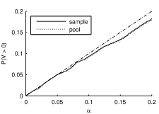
(a) Col

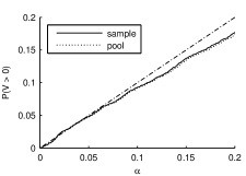
(b) Swap

Figure 10: minP test for different $p$-value calculation and randomization methods with Paleo. The true FWER is plotted against the controlled level. The diagonal dash-dotted line should not be exceeded for the minP-property to be satisfied.

[h]

(a) Col

(b) Swap

Figure 11: minP test for different $p$-value calculation and randomization methods with Courses. The true FWER is plotted against the controlled level. The diagonal dash-dotted line should not be exceeded for the minP-property to be satisfied.

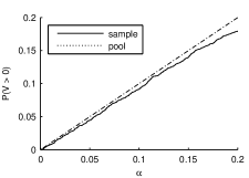
(a) Col

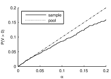
(b) Swap

Figure 12: minP test for different $p$-value calculation and randomization methods with Retail. The true FWER is plotted against the controlled level. The diagonal dash-dotted line should not be exceeded for the minP-property to be satisfied.

References

- [1] Stephen D. Bay and Michael J. Pazzani. Detecting group differences: Mining contrast sets. Data Min. Knowl. Discov., 5(3):213–246, 2001.
- [2] Yoav Benjamini and Yosef Hochberg. Controlling the false discovery rate: A practical and powerful approach to multiple testing. Journal of the Royal Statistical Society. Series B (Methodological), 57(1):289–300, 1995.
- [3] Yoav Benjamini and Daniel Yekutieli. The control of the false discovery rate in multiple testing under dependency. The Annals of Statistics, 29(4):1165–1188, 2001.
- [4] Sandrine Dudoit, Juliet Popper Shaffer, and Jennifer C. Boldrick. Multiple hypothesis testing in microarray experiments. Statistical Science, 18(1):71–103, 2003.
- [5] Aristides Gionis, Heikki Mannila, Taneli Mielikäinen, and Panayiotis Tsaparas. Assessing data mining results via swap randomization. In Proceedings of the 12th ACM Conference on Knowledge Discovery and Data Mining (KDD), 2006.
- [6] Sami Hanhijärvi, Gemma C. Garriga, and Kai Puolamäki. Randomization techniques for graphs. In Proceedings of the 2009 SIAM International Conference on Data Mining (SDM 09), 2009.
- [7] S. Holm. A simple sequentially rejective multiple test procedure. Scandinavian Journal of Statistics, 6:65–70, 1979.
- [8] Michihiro Kuramochi and George Karypis. An efficient algorithm for discovering frequent subgraphs. IEEE Trans. Knowl. Data Eng., 16(9):1038–1051, 2004.
- [9] St phane Lallich, Olivier Teytaud, and Elie Prudhomme. Association rule interestingness: measure and statistical validation. Quality Measures in Data Mining, pages 251–275, 2006.
- [10] St phane Lallich, Olivier Teytaud, and Elie Prudhomme. Statistical inference and data mining: false discoveries control. In 17th COMPSTAT Symposium of the IASC, La Sapienza, Rome, pages 325–336, 2006.
- [11] E. L. Lehmann. Testing Statistical Hypotheses. Wiley, 1956.
- [12] Ruth Marcus, Eric Peritz, and K. R. Gabriel. On closed testing procedures with special reference to ordered analysis of variance. Biometrica, 63(3):655–660, 1976.
- [13] Nimrod Megiddo and Ramakrishnan Srikant. Discovering predictive association rules. In Knowledge Discovery and Data Mining, pages 274–278, 1998.
- [14] B. V. North, D. Curtis, and P. C. Sham. A note on the calculation of empirical P values from Monte Carlo procedures. The American Journal of Human Genetics, 71(2):439–441, 2002.
- [15] Markus Ojala, Niko Vuokko, Aleksi Kallio, Niina Haiminen, and Heikki Mannila. Randomization of real-valued matrices for assessing the significance of data mining results. In Proceedings of the 2008 SIAM International Conference on Data Mining, pages 494–505, 2008.
- [16] Roded Sharan, Trey Ideker, Brian Kelley, Ron Shamir, and Richard M. Karp. Identification of protein complexes by comparative analysis of yeast and bacterial protein interaction data. Journal of Computational Biology, 12(6):835–846, 2005.
- [17] Geoffrey I. Webb. Discovering significant rules. In KDD ’06: Proceedings of the 12th ACM SIGKDD international conference on Knowledge discovery and data mining, pages 434–443, New York, NY, USA, 2006. ACM.
- [18] Geoffrey I. Webb. Discovering significant patterns. Mach. Learn., 68(1):1–33, 2007.
- [19] Peter H. Westfall and S. Stanley Young. Resampling-based multiple testing: examples and methods for p-value adjustment. Wiley, 1993.
- [20] Hong Zhang, Balaji Padmanabhan, and Alexander Tuzhilin. On the discovery of significant statistical quantitative rules. In KDD ’04: Proceedings of the tenth ACM SIGKDD international conference on Knowledge discovery and data mining, pages 374–383, New York, NY, USA, 2004. ACM.