ON THE STATICS AND DYNAMICS OF MAGNETO-ANISOTROPIC NANOPARTICLES

I Introduction

Small, magnetically ordered particles, are ubiquitous both in naturally occurring and manufactured forms. On the one hand, it is remarkable the wide spectrum of applications of these systems, which range from magnetic recording media, catalysts, magnetic fluids, filtering and phase separation in mineral processing industry, magnetic imaging and magnetic refrigeration, to numerous geophysical, biological, and medical uses. On the other hand, the nanometric magnetic particles can be considered as model systems for the study of various basic physical phenomena. Among others we can mention: rotational Brownian motion and thermally activated processes in multistable systems, mesoscopic quantum phenomena, dipole-dipole interaction effects, and the dependence of the properties of solids on their size.

Magnetically ordered particles of nanometric size generally consist of a single domain, whose constituent spins, at temperatures well below the Curie temperature, rotate in unison. The magnetic energy of a nanometric particle is then determined by its magnetic moment orientation, and has a number of stable directions separated by potential barriers (associated with the magnetic anisotropy). As a result of the coupling of the magnetic moment of the particle, $\vec{m}$, with the microscopic degrees of freedom of its environment (phonons, conducting electrons, nuclear spins, etc.), the magnetic moment is subjected to thermal fluctuations and may undergo a Brownian-type rotation surmounting the potential barriers. This solid-state relaxation process was proposed and studied by Néel (1949), and subsequently reexamined by Brown (1963), by dint of the theory of stochastic processes.

In the high potential-barrier range, $\Delta U/k_{{\rm B}}T\gg 1$, the characteristic time for the over-barrier rotation process, $\tau_{\|}$, can approximately be written in the Arrhenius form $\tau_{\|}\simeq\tau_{0}\exp(\Delta U/k_{{\rm B}}T)$, where $\tau_{0}$ ($\sim 10^{-10}$–$10^{-12}$ s) is related with the intra-potential-well dynamics. For $\tau_{\|}\ll t_{{\rm m}}$ ($t_{{\rm m}}$ is the measurement or observation time), $\vec{m}$ maintains the equilibrium distribution of orientations as in a classical paramagnet; because $m=|\vec{m}|$ is much larger than a typical microscopic magnetic moment ($m\sim 10^{3}$–$10^{5}\,\mu_{{\rm B}}$) this phenomenon is named superparamagnetism. In contrast, when $\tau_{\|}\gg t_{{\rm m}}$, the magnetic moment rotates rapidly about a potential minimum whereas the over-barrier relaxation mechanism is blocked. This corresponds to the state of stable magnetization in a bulk magnet. Finally, under intermediate conditions ($\tau_{\|}\sim t_{{\rm m}}$) non-equilibrium phenomena, accompanied by magnetic “relaxation,” are observed. It is to be noted that, in the Arrhenius range mentioned, the system may pass through all these regimes in a relatively narrow temperature interval.

We shall describe a nanoparticle as a classical magnetic moment with magnetic-anisotropy energy. This brings generality to the results and the connection with other physical systems that can approximately be described as ensembles of “rotators” in certain orientational potentials. Examples include: molecular magnetic clusters with high spin in their ground state (in the ranges where a classical description of their spins is reasonable); nematic liquid crystals with uniaxial physical properties; relaxor ferroelectrics; certain high-spin dilutely-doped glasses described by the random-axial-anisotropy model; and superparamagnetic-like spin glasses.

Indeed, the analogies between the macroscopic behavior of certain electric and magnetic “glassy” systems and that of ensembles of small magnetic particles have received recurrent attention during the last 20 years. The magnetic nanoparticle systems exhibit glassy-like phenomena associated with the distribution of particle parameters (anisotropy constants, volumes, magnetic moments, etc.), which lead to more or less wide distributions of relaxation times. On the other hand, ensembles of interacting nanoparticles apparently exhibit genuine glassy properties, mainly due to the extremely anisotropic character of the dipole-dipole interaction. Therefore, it is important to determine which phenomena are intrinsically due to the presence of interactions in the nanoparticle ensemble and which others not. In this connection, owing to the lack of enough knowledge about some of the properties of independent magnetic particles, it is not always known from which “laws” the corresponding quantities depart as a consequence of the inter-particle interactions. Similar considerations also apply to the study of the effects associated with quantum phenomena in small magnetic particles; as complete a knowledge as possible of the classical regime is the mandatory starting point towards the study of, for example, quantum tunnelling and coherence in these systems.

Finally, the study of the dynamics of non-interacting classical magnetic moments is an interesting strand of research per se, which seems to be far from exhausted. Indeed, relevant developments of the pioneering works of the 1960s and 1970s have been performed during the last 15 years.

The purpose of this Chapter is to gain a deeper insight into the statical (thermal-equilibrium) and dynamical (non-equilibrium) properties of non-interacting magnetically anisotropic nanoparticles in the framework of classical physics.

The scheme followed in this work is as follows: In Sections II and III some thermal-equilibrium properties of classical magnetic moments are studied. Section II is devoted to the obtainment of general results for the basic thermodynamical functions (partition function and thermodynamical potentials), some of which are subsequently used in Section III to calculate various important thermal-equilibrium quantities. Some known results are reobtained (presenting in some cases alternative expressions and/or derivations), whereas the superparamagnetic theory is extended by calculating a number of other quantities. The central issue along these first two Sections is the study of the effects of the magnetic anisotropy on the thermal-equilibrium properties of superparamagnetic systems. These effects are sometimes ignored because superparamagnetism is restrictively associated with the temperature range where the anisotropy energy is smaller than the thermal energy.

In the remainder Sections we shall concentrate on the dynamical properties of classical magnetic moments. The heuristic approach to the dynamics of these systems is considered in Section IV, where the analyses of the corresponding models in order to extract certain parameters of ensembles of magnetic nanoparticles are revised and developed. In Section V the dynamical properties of classical magnetic moments are studied by the methods of the theory of stochastic processes. The Brown–Kubo–Hashitsume stochastic model is presented in a unified way and Langevin-dynamics simulations are performed to study the non-zero temperature dynamical properties. Both the study of individual stochastic trajectories and the response of ensembles of magnetic moments are undertaken. Finally, Section VI is devoted to the foundation of the dynamical equations that are the basis of Section V. The techniques of the formalism of the independent-oscillator environment are employed to derive dynamical equations for the magnetic moment that take the effects of its interaction with the surrounding medium into account.

II Equilibrium properties: generalities and methodology

II.A Introduction

Throughout this Chapter we shall concentrate on the study of magnetic moments whose physical support (the crystal lattice in magnetic nanoparticles), to which they are linked by the magnetic anisotropy, is fastened in space. In small-particle magnetism, this corresponds to particles dispersed in a solid matrix. Although this apparently excludes the so called “magnetic fluids” (where the physical rotation of the particles plays a fundamental rôle), these belong to the class of solid dispersions when the liquid carrier is frozen (which is besides the case of experimental interest when studying low-temperature properties). On the other hand, we shall also restrict our study to systems with axially symmetric magnetic anisotropy. This choice makes the problem mathematically tractable and provides valuable insight into more complex situations.

As was mentioned in Section I, the thermal-equilibrium (superparamagnetic) behavior is observed when the measurement or observation time, $t_{{\rm m}}$, is much longer than the characteristic relaxation times of the system (this is of course a general statement). In Table I the measurement times of various experimental techniques are displayed.

Note that the thermal-equilibrium range can extend down to temperatures where the heights of the energy barriers (created by the magnetic anisotropy) are much larger than the thermal energy. To illustrate, for a system with an axially symmetric Hamiltonian and in the high-barrier range, the mean time for the over-barrier rotation process, $\tau_{\|}$, can be written in the Arrhenius form

$$\tau_{\|}=\tau_{0}\exp(\Delta U/k_{{\rm B}}T)\;.$$ (2.1)

Besides, the “high-barrier” range where this expression for the relaxation time holds, extends down to $\Delta U/k_{{\rm B}}T\,\raisebox{1.50696pt}{$>$}\raisebox{-2.79857pt}{$\sim$}\,2$; moreover, for $\Delta U/k_{{\rm B}}T\,\raisebox{1.50696pt}{$<$}\raisebox{-2.79857pt}{$\sim$}\,2$, the relaxation time $\tau_{\|}$ is of the order of $\tau_{0}$ ($\sim 10^{-10}$–$10^{-12}$ s for magnetic nanoparticles). Therefore, the exponential decrease of $\tau_{\|}$ as $T$ increases, yields the range

$$\ln(t_{{\rm m}}/\tau_{0})>\Delta U/k_{{\rm B}}T\geq 0\;,$$

as the thermal-equilibrium range ($\tau_{\|}\ll t_{{\rm m}}$) for a given measurement time $t_{{\rm m}}$. For instance, for magnetic measurements with $t_{{\rm m}}\sim 1$–$100$ s, this range is extremely wide ($25>\Delta U/k_{{\rm B}}T\geq 0$). This entails that the frequently encountered statement, “superparamagnetism occurs when the thermal energy is comparable or larger than the energy barriers”, is unnecessarily restrictive.

TABLE I.: Characteristic measurement times of various experimental techniques.

Experimental technique	Measurement time
magnetization	$1$–$100$ s
ac susceptibility	$10^{-6}$–$100$ s
Mössbauer spectroscopy	$10^{-9}$–$10^{-7}$ s
Ferromagnetic resonance	$10^{-9}$ s
Neutron scattering	$10^{-12}$–$10^{-8}$ s

Let us further illustrate this important point which rests essentially on the magnitude of $\tau_{0}$ and the exponential dependence of $\tau_{\|}$ on $T$ in Eq. (2.1). For an experiment with measurement time $t_{{\rm m}}$, the blocking temperature, $T_{{\rm b}}$, defined as the temperature where $t_{{\rm m}}=\tau_{\|}$, is given by $t_{{\rm m}}=\tau_{0}\exp(\Delta U/k_{{\rm B}}T_{{\rm b}})$. Accordingly, one has $\ln(t_{{\rm m}}/\tau_{0})=\Delta U/k_{{\rm B}}T_{{\rm b}}$ so that, if $t_{{\rm m}}=\tau_{0}10^{12}$ (a typical value for standard magnetic measurements), it follows that $\Delta U/k_{{\rm B}}T_{{\rm b}}=\ln(10^{12})\simeq 27.6$. However, for $\Delta U/(k_{{\rm B}}1.1T_{{\rm b}})\simeq 25$, one already finds $\tau_{\|}=0.08t_{{\rm m}}$ while for $\Delta U/(k_{{\rm B}}1.2T_{{\rm b}})\simeq 23$, one has $\tau_{\|}=0.01t_{{\rm m}}$, i.e., the system is clearly in the thermal-equilibrium regime, whereas $\Delta U$ is still much larger than $k_{{\rm B}}T$.

Thus, there exists an extremely wide range where superparamagnetism occurs ($\tau_{\|}\ll t_{{\rm m}}$) and, simultaneously, the “naïve condition of superparamagnetism” $\Delta U/k_{{\rm B}}T\,\raisebox{1.50696pt}{$<$}\raisebox{-2.79857pt}{$\sim$}\,1$, is not necessarily obeyed. Consequently, in that range, the effects of the anisotropy-energy on the equilibrium quantities can be sizable. Indeed, for any thermal-equilibrium quantity, prior to the observation of the corresponding “blocking” (departure from thermal-equilibrium behavior) when the temperature is sufficiently lowered, one can clearly observe a crossover from the isotropic-type behavior at high temperatures (where the anisotropy potential plays a minor rôle) to either a discrete-orientation- or plane-rotator-type behavior at low temperatures (where the magnetic moment stays most of the time in the potential-minima regions), without leaving the thermal-equilibrium range.

The organization of the remainder of this Section is as follows. In Subsec. II.B we shall introduce and discuss the Hamiltonian for a small magnetic particle. In Subsec. II.C the partition function and free energy are introduced. In Subsec. II.D we shall carry out the expansion of the partition function in powers of either the external field or the anisotropy constant, along with an asymptotic expansion for strong anisotropy. Finally, in Subsec. II.E, we shall derive the corresponding expansions of the free energy.

II.B Hamiltonian

To begin with, we shall discuss the concept of effective Hamiltonian for a small, magnetically ordered particle. Then we shall introduce the basic form of the Hamiltonian that will be studied along this work, to conclude with the study of the energy barriers in the longitudinal-field case.

1. Effective Hamiltonian of a nanoparticle

A basic assumption in small-particle magnetism is that a single-domain particle, with a given physical orientation, is in internal thermodynamical equilibrium at temperature $T$. Not too close to the Curie temperature, its constituent spins rotate in unison (coherent rotation), so the only relevant degree of freedom left is the orientation of the net magnetic moment. With respect to this variable the thermal equilibration can take place in a time scale that can be considerably longer than that of the internal equilibration. Under such conditions, the internal free energy (for a given instantaneous orientation) can be considered as an effective energy (Hamiltonian) for the orientational degrees of freedom.

The consideration of a internal free energy as an effective Hamiltonian for the remainder degrees of freedom is indeed general, and it is founded in the very statistical-mechanical definition of the free energy. Let $(p,q)$ be the canonical variables “of interest” and $({\bf P},{\bf Q})$ the set of “internal” variables. The partition function, ${\cal Z}$, and the free energy, ${\cal F}$, are defined in terms of the total Hamiltonian of the system, ${\cal H}_{\rm T}$, as

$${\cal Z}=\int\!\!{\rm d}p{\rm d}q{\rm d}{\bf P}{\rm d}{\bf Q}\,\exp[-\beta{\cal H}_{\rm T}(p,q;{\bf P},{\bf Q})]\;,\qquad{\cal F}=-\frac{1}{\beta}\ln{\cal Z}\;,$$

where $\beta=1/k_{{\rm B}}T$. One can define internal quantities for given values of the variables $p$ and $q$ (marked by a tilde), as follows

$$\tilde{{\cal Z}}(p,q)=\int\!\!{\rm d}{\bf P}{\rm d}{\bf Q}\,\exp[-\beta{\cal H}_{\rm T}(p,q;{\bf P},{\bf Q})]\;,\qquad\tilde{{\cal F}}(p,q)=-\frac{1}{\beta}\ln\tilde{{\cal Z}}(p,q)\;.$$

Note that, by definition, the internal free energy obeys the relation

$$\exp[-\beta\tilde{{\cal F}}(p,q)]=\int\!\!{\rm d}{\bf P}{\rm d}{\bf Q}\,\exp[-\beta{\cal H}_{\rm T}(p,q;{\bf P},{\bf Q})]\;.$$

Therefore, the total partition function ${\cal Z}$, from which all the equilibrium quantities of the system can be derived, can be written as

$${\cal Z}=\int\!\!{\rm d}p{\rm d}q\exp[-\beta\tilde{{\cal F}}(p,q)]\;.$$

This equation demonstrates the above statement: the so-defined internal free energy $\tilde{{\cal F}}(p,q)$ plays the rôle of an effective Hamiltonian for the variables $p$ and $q$ when studying the equilibrium properties of the system. Note that this effective Hamiltonian may have, by its very definition, terms dependent on $T$.

Naturally, this approach is in principle applicable to any chosen pair of variables $(p,q)$. However, for this procedure to be useful, a time-scale separation between some internal “fast” variables and certain “slow” ones must occur. In our case, the orientation of the total magnetic moment plays the rôle of the latter and, in what follows, we shall refer to the so-introduced internal free energy as the magnetic energy (Hamiltonian) of the nanoparticle, and it will be simply denoted by ${\cal H}(\vec{m})$.

Similar considerations can, in principle, be applied to a magnetic domain in a bulk magnet but, for such a macroscopic system, the time scale separation mentioned is so huge that the probability of thermally activated magnetization reversal is almost zero over astronomical time scales; the system is then effectively confined in a restricted region of the phase space. Note finally that the separation procedure between “internal” and “relevant” variables would lead to exact results if one in fact uses the above definitions to calculate $\tilde{{\cal F}}(p,q)$ by “integrating out” the internal variables. However, this is not possible in general, but one determines $\tilde{{\cal F}}(p,q)$ on the basis of series truncations, symmetry arguments, etc. (Brown, 1979).

2. Hamiltonian studied

The magnetic energy of a nanoparticle has a number of different contributions, e.g., magnetostatic self-energy (“demagnetization” or “shape” energy), magneto-crystalline energy, surface terms, magneto-elastic energy, etc. All these contributions give rise to a dependence of the energy of the nanoparticle on the orientation of its magnetic moment, i.e., in the absence of an external magnetic field the magnetic properties of the system are anisotropic. We shall mainly consider systems where the magnetic-anisotropy energy has the simplest axial symmetry. Then, if an external field $\vec{B}$ is applied (assumed to be uniform over the volume of the system), the total magnetic energy reads

$${\cal H}(\vec{m})=-\frac{Kv}{m^{2}}(\vec{m}\cdot\hat{n})^{2}-\vec{m}\cdot\vec{B}\;,$$ (2.2)

where $K$ is the magnetic-anisotropy energy constant, $v$ is the volume of the nanoparticle, and $\hat{n}$ is a unit vector along the symmetry axis of the magnetic-anisotropy term (hereafter referred to as the anisotropy axis).

On introducing the unit vectors $\vec{e}$, in the direction of the magnetic moment ($\vec{e}=\vec{m}/m$), and $\hat{b}$, in the direction of the external magnetic field ($\hat{b}=\vec{B}/B$), as well as the dimensionless anisotropy and field parameters

$$\sigma=\frac{Kv}{k_{{\rm B}}T}\;,\qquad\xi=\frac{mB}{k_{{\rm B}}T}\;,$$ (2.3)

the Hamiltonian (2.2) can be written as

$$-\beta{\cal H}=\sigma(\vec{e}\cdot\hat{n})^{2}+\xi(\vec{e}\cdot\hat{b})\;.$$ (2.4)

For $K>0$ the anisotropy is of “easy-axis” type, since the two existing minima of the anisotropy term point along $\pm\hat{n}$ (the “poles”). On the other hand, for $K<0$ the anisotropy is of “easy-plane” type, the minima of the anisotropy term being then continuously distributed over the plane perpendicular to $\hat{n}$ (the “equatorial” region).

The adopted expression for the magnetic anisotropy is the leading term in the expansion of a general uniaxial magneto-crystalline anisotropy energy with respect to the direction cosines of the magnetization. On the other hand, such a form is also the appropriate one for shape anisotropy (demagnetization self-energy) of an ellipsoid of revolution

$${\cal H}_{{\rm dem}}={\textstyle\frac{1}{2}}v\mu_{0}M_{s}^{2}\left(D_{a}\cos^{2}\!\vartheta+D_{b}\sin^{2}\!\vartheta\right)\;,$$

where $\vartheta$ is the angle between the magnetic moment and the long (polar) axis of the ellipsoid, $M_{s}=m/v$ is the spontaneous magnetization, $D_{a}$ the demagnetization factor along the polar axis, and $D_{b}$ the demagnetization factor along an equatorial axis. Indeed, we can write the above expression as ${\cal H}_{{\rm dem}}={\rm cte}-{\textstyle\frac{1}{2}}v\mu_{0}M_{s}^{2}\left(D_{b}-D_{a}\right)\cos^{2}\!\vartheta$, so that the corresponding anisotropy constant reads

$$K_{{\rm dem}}={\textstyle\frac{1}{2}}\mu_{0}M_{s}^{2}\left(D_{b}-D_{a}\right)\;.$$ (2.5)

In this case easy-axis and easy-plane anisotropy correspond, respectively, to prolate and oblate ellipsoids of revolution.

For many materials, slight deviations from spherical shape make the shape anisotropy to dominate the remainder contributions to the magnetic anisotropy. On the other hand, as was shown by Brown and Morrish (1957), a single-domain particle with an arbitrary shape is equivalent to a suitably chosen general ellipsoid, as far as the behavior of its magnetization in a uniform applied field is concerned. Therefore, after these results, the seemingly specialized study of ellipsoids of revolution (i.e., of uniaxial anisotropy) can be of great importance to account for the effects of a general shape anisotropy.

In what follows we shall phrase our discussion in the language of classical magnetic moments. Nevertheless, the results obtained will be applicable to systems consisting of classical dipole moments that could approximately be described by Hamiltonians akin to (2.2), i.e., Hamiltonians comprising a coupling term to an (electric or magnetic) external field plus an axially symmetric orientational potential.

3. Energy barriers in the longitudinal-field case

We shall now study the behavior of the Hamiltonian in the illustrative $\vec{B}\parallel\hat{n}$ case, determining its extrema and how they change as a function of the several parameters in the Hamiltonian.

Before proceeding, let us introduce two useful quantities: the maximum anisotropy field, $B_{K}$, and $h$, the external field measured in units of $B_{K}$,

$$B_{K}=\frac{2Kv}{m}\;,\qquad h=\frac{B}{B_{K}}=\frac{\xi}{2\sigma}\;.$$ (2.6)

Let us now write the energy in terms of $\sigma$, the reduced field $h$, and the angle $\vartheta$ between $\vec{m}$ and the anisotropy axis [cf. Eq. (2.4)]

$$\beta{\cal H}=-\sigma(\cos^{2}\!\vartheta+2h\cos\vartheta)\;.$$ (2.7)

To fix ideas, we shall assume $\sigma>0$, i.e., anisotropy of easy-axis type. The results for $\sigma<0$, will be analogous but what is a maximum for $\sigma>0$, becomes a minimum for $\sigma<0$, and vice-versa. The extrema of ${\cal H}$ are obtained by equating to zero the $\vartheta$-derivative $\partial(\beta{\cal H})/\partial\vartheta=2\sigma\sin\vartheta(\cos\vartheta+h)$ getting

$$\frac{\partial(\beta{\cal H})}{\partial\vartheta}=0\quad\Longrightarrow\quad\left\{\begin{array}[]{lcl}\sin\vartheta=0&\Leftrightarrow&\vartheta=0,\pi\\ \cos\vartheta=-h&\mbox{if}&|h|\leq 1\end{array}\right.\;.$$

The type of extrema is obtained by evaluating the second derivative at the extrema:

$$\frac{\partial{}^{2}(\beta{\cal H})}{\partial\vartheta^{2}}=\left\{\begin{array}[]{ll}\;\;\;2\sigma(1+h)&\mbox{ for }\vartheta=0\\ \;\;\;2\sigma(1-h)&\mbox{ for }\vartheta=\pi\\ -2\sigma(1-h^{2})&\mbox{ for }\cos\vartheta=-h\quad(\mbox{if~{}}|h|\leq 1)\end{array}\right.\;,$$

so that one gets the following results

	minima	maxima
$|h|<1$	$\vartheta=0,\pi$	$\vartheta=\arccos(-h)$
$h>1$	$\vartheta=0$	$\vartheta=\pi$
$h<-1$	$\vartheta=\pi$	$\vartheta=0$

Thus, for $|h|<1$ (i.e., for $|B|<B_{K}$), the energy has minima at $\vartheta=0$ and $\vartheta=\pi$, with a maximum between them (see the upper panel of Fig. 1). On the other hand, for $|h|>1$ (that is, for fields higher than the maximum anisotropy field $B_{K}$), the upper (shallower) energy minimum ($\vartheta=\pi$ for $h>0$) turns into a maximum as it merges with the intermediate maximum, which disappears (lower panel of Fig. 1).

FIGURE 1.: Magnetic energy in the longitudinal-field case for a number of values of the reduced field parameter $h=B/B_{K}$. Upper panel: $0\leq h<1$, so that the potential has two minima with an energy-barrier between them. Lower panel: $h\geq 1$, so that no potential barrier exists.

Finally, from the values of the energy at $\vartheta=0,\pi$, and, when it exists, at the intermediate maximum $\vartheta_{\rm M}=\arccos(-h)$, one gets the energy-barrier heights ($|h|<1$)

$$\beta[{\cal H}(\vartheta_{\rm M})-{\cal H}(0)]=\sigma_{+}\;,\qquad\beta[{\cal H}(\vartheta_{\rm M})-{\cal H}(\pi)]=\sigma_{-}\;,$$

where

$$\sigma_{\pm}=\sigma(1\pm h)^{2}\;.$$ (2.8)

II.C Partition function and free energy

1. General definitions

The statistical independence of non-interacting magnetic moments allows one to express the thermodynamical quantities as sums over one-dipole contributions. Consequently, we shall study these contributions and the results for the whole system will be obtained by summation (or integration) of them over the ensemble of dipoles, taking their different anisotropy constants, orientations about the external field, magnitude of their dipole moments, etc. into account.

The partition function associated with a Hamiltonian ${\cal H}(\vartheta,\varphi)$, where $\vartheta,\varphi$ are the angular coordinates of $\vec{m}$ in a spherical coordinate system, can be defined as

$${\cal Z}=\frac{1}{2\pi}\int_{0}^{\pi}\!\!{\rm d}{\vartheta}\,\sin\vartheta\int_{0}^{2\pi}\!\!{\rm d}{\varphi}\,\exp[-\beta{\cal H}(\vartheta,\varphi)]\;,$$ (2.9)

while the associated free energy is then given by

$${\cal F}=-k_{{\rm B}}T\ln{\cal Z}\;.$$

The definition (2.9) deserves some discussion. First, as was mentioned above, the definition of the partition function for a system with one degree of freedom is ${\cal Z}=\int({\rm d}p{\rm d}q/2\pi\hbar)\exp(-\beta{\cal H})$ (Landau and Lifshitz, 1980, § 31). On the other hand, for a classical magnetic moment a convenient pair of conjugate canonical variables is $p=m_{z}/\gamma$ and $q=\varphi$ [see Eq. (6.11) in Section VI], where $m_{z}=m\cos\vartheta$ and $\gamma$ is the gyromagnetic (or rather “magnetogyric”) ratio. Therefore

$$\int\frac{{\rm d}p{\rm d}q}{2\pi\hbar}(\cdot)=\frac{m}{\gamma\hbar}\frac{1}{2\pi}\int_{-1}^{1}\!\!{\rm d}{(\cos\vartheta)}\,\int_{0}^{2\pi}\!\!{\rm d}{\varphi}\,(\cdot)=S\times\frac{1}{2\pi}\int_{0}^{\pi}\!\!{\rm d}{\vartheta}\,\sin\vartheta\int_{0}^{2\pi}\!\!{\rm d}{\varphi}\,(\cdot)\;,$$

where $S=(m/\gamma)/\hbar$ is the quantum number associated with the angular momentum $m/\gamma$. This expression yields ${\cal Z}=2S$ for ${\cal H}\equiv 0$, which is the correct semiclassical case ($S\gg 1$) of the corresponding quantum expression ${\cal Z}=\sum_{S_{z}=-S}^{S}1=2S+1$. Therefore the definition (2.9) corresponds to the proper statistical-mechanical definition, except for the factor $S$, which when required can be introduced by hand.

The equilibrium probability distribution of magnetic moment orientations is given by the Boltzmann distribution

$$P_{{\rm e}}(\cos\vartheta,\varphi)={\cal Z}^{-1}\exp[-\beta{\cal H}(\vartheta,\varphi)]\;,$$

so that the statistical-mechanical average of any observable $A=A(\vec{m})=A(\vartheta,\varphi)$ reads

$$\left\langle A\right\rangle_{{\rm e}}=\int\!\!{\rm d}{\Omega}\,A(\vartheta,\varphi)P_{{\rm e}}(\vartheta,\varphi)=\frac{\int\!{\rm d}{\Omega}\,A(\vartheta,\varphi)\exp[-\beta{\cal H}(\vartheta,\varphi)]}{\int\!{\rm d}{\Omega}\,\exp[-\beta{\cal H}(\vartheta,\varphi)]}\;,$$ (2.10)

where $\int\!{\rm d}{\Omega}\,(\cdot)\equiv(1/2\pi)\int_{-1}^{1}\!{\rm d}{(\cos\vartheta)}\,\int_{0}^{2\pi}\!{\rm d}{\varphi}\,(\cdot)$. The relevant thermodynamical quantities can be written as the statistical-mechanical average of a certain function $A=A(\vartheta,\varphi)$ as above. Besides, all of them can be obtained as combinations of ${\cal Z}$ (or ${\cal F}$) and its derivatives. Table II summarizes some of these celebrated relations, which illustrate the pivotal rôle that the calculation of the partition function (or the free energy) plays in equilibrium statistical mechanics.

TABLE II.: Definition of various thermodynamical quantities and their expressions in terms of the partition function ${\cal Z}$, and of the free energy ${\cal F}$.

	$\quad{\cal A}\quad$	def.	${\cal A}({\cal Z})$	${\cal A}({\cal F})$
energy	${\cal U}$	$\left\langle{\cal H}\right\rangle_{{\rm e}}$	$-\frac{\partial{}}{\partial\beta}(\ln{\cal Z})$	${\cal F}+\beta\frac{\partial{}}{\partial\beta}{\cal F}$
entropy	${\cal S}$	$-\left\langle\ln P_{{\rm e}}\right\rangle_{{\rm e}}$	$\ln{\cal Z}-\beta\frac{\partial{}}{\partial\beta}(\ln{\cal Z})$	$\beta^{2}\frac{\partial{}}{\partial\beta}{\cal F}$
magnetization	$M_{B}$	$\big{\langle}\vec{m}\cdot\hat{b}\big{\rangle}_{{\rm e}}$	$m\frac{\partial{}}{\partial\xi}(\ln{\cal Z})$	$-m\beta\frac{\partial{}}{\partial\xi}{\cal F}$

2. Partition function for the simplest axially symmetric anisotropy potential

We shall usually choose the anisotropy axis $\hat{n}$ as the polar axis of a spherical coordinate system. Then, if $(\vartheta,\varphi)$ and $(\alpha,0)$ denote the angular coordinates of $\vec{m}$ and $\vec{B}$, respectively (see Fig. 2), the Hamiltonian (2.4) reads

$$-\beta{\cal H}=\sigma\cos^{2}\!\vartheta+\xi_{\|}\cos\vartheta+\xi_{\perp}\sin\vartheta\cos\varphi\;,$$ (2.11)

where we have introduced the longitudinal and transverse components (with respect to the anisotropy-axis direction) of the dimensionless field $\vec{\xi}=m\vec{B}/k_{{\rm B}}T$, namely

$$\xi_{\|}=\xi\cos\alpha\;,\qquad\xi_{\perp}=\xi\sin\alpha\;.$$ (2.12)

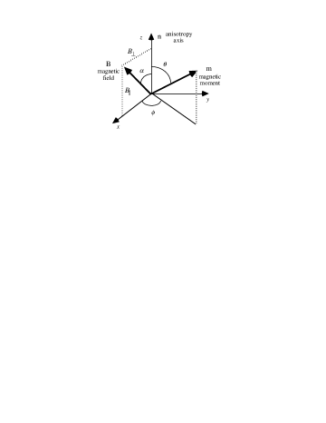
FIGURE 2.: Coordinate system used in the calculation of the thermal-equilibrium quantities. The plane determined by $\hat{n}$ and $\vec{B}$ is chosen as the $xz$-plane.

In order to analyze the partition function we, following Shcherbakova (1978), do first the integral over $\varphi$ in the expression for ${\cal Z}$ associated with the Hamiltonian (2.11), getting

$${\cal Z}=\int_{0}^{\pi}\!\!{\rm d}{\vartheta}\,\sin\vartheta\exp(\sigma\cos^{2}\!\vartheta+\xi_{\|}\cos\vartheta)I_{0}(\xi_{\perp}\sin\vartheta)\;,$$ (2.13)

where

$$I_{n}(y)=\frac{1}{\pi}\int_{0}^{\pi}\!\!{\rm d}{t}\,e^{y\cos t}\cos nt=\sum_{k=0}^{\infty}\frac{1}{k!(k+n)!}\left(\frac{y}{2}\right)^{2k+n},\quad n\geq 0\;,$$ (2.14)

is the modified Bessel function of the first kind of order $n$ (see, for example, Arfken, 1985, Sect. 11.5).

Equation (2.13) gives the partition function in terms of an integral over $\vartheta$ only. Therefore, the integrand (divided by ${\cal Z}$) can be interpreted as an effective probability distribution of the polar angle. Indeed, on introducing the substitution $z=\cos\vartheta$ one can first write Eq. (2.13) as

$${\cal Z}=\int_{-1}^{1}\!\!{\rm d}{z}\,\exp(\sigma z^{2}+\xi_{\|}z)I_{0}(\xi_{\perp}\sqrt{1-z^{2}})\;.$$ (2.15)

Then, the thermal-equilibrium average of functions of $\cos\vartheta$ only can be obtained through $\langle A\rangle_{{\rm e}}=\int_{-1}^{1}\!{\rm d}{z}\,A(z)P_{{\rm e}}^{{\rm eff}}(z)$ where

$$P_{{\rm e}}^{{\rm eff}}(z)=\frac{1}{{\cal Z}}\exp(\sigma z^{2}+\xi_{\|}z)I_{0}(\xi_{\perp}\sqrt{1-z^{2}})\;,$$ (2.16)

is the effective or averaged (over the azimuthal angle), probability distribution. Naturally $P_{{\rm e}}^{{\rm eff}}(z)$ coincides with the actual probability distribution when the total ${\cal H}(\vec{m})$ is axially symmetric.

3. Particular cases and limiting regimes

In various special cases, one can write down the partition function and the free energy in a closed analytical form. Accordingly, along with being relevant to get insight into the thermal-equilibrium properties of the system, these expressions will be used as reference for the general or approximate formulae derived along this Section.

a. Isotropic case.

We shall first consider the case $\sigma=0$. This isotropic or Langevin regime will be attained if the anisotropy constant is identically zero or at high temperatures where $|\sigma|\ll 1$. Then, the partition function does not depend on $\alpha$ ($\cos\alpha=\hat{n}\cdot\hat{b}$), so we can choose $\alpha$ at will in Eq. (2.15). On setting $\alpha=0$ (so that $\xi_{\perp}=0$ and $\xi_{\|}=\xi$) and using $I_{0}(0)=1$, equation (2.15) reduces to ${\cal Z}_{{\rm Lan}}=\int_{-1}^{1}\!{\rm d}{z}\,\exp(\xi z)$. Therefore, the partition function and free energy in the isotropic case can be written as

$${\cal Z}_{{\rm Lan}}=\frac{2}{\xi}\sinh\xi\;,\qquad{\cal F}_{{\rm Lan}}=k_{{\rm B}}T[\ln(\xi)-\ln(2\sinh\xi)]\;.$$ (2.17)

Similarly, the probability distribution (2.16) reduces in this case to

$$P_{{\rm e},{\rm Lan}}(z)=\frac{\exp(\xi z)}{(2/\xi)\sinh\xi}\;,$$ (2.18)

which is is displayed in Fig. 3

FIGURE 3.: Probability distribution of the $z$ component of the magnetic moment for $\sigma=Kv/k_{{\rm B}}T=0$ in a magnetic field [Eq. (2.18)], for various values of the dimensionless field parameter $\xi=mB/k_{{\rm B}}T$. The value $0.5$ corresponds to the uniform probability distribution ($\sigma=\xi=0$).

b. Zero-field case.

In the absence of an external field (unbiased case), one can use again $I_{0}(0)=1$ in Eq. (2.15), to get ${\cal Z}_{{\rm unb}}=2\int_{0}^{1}\!{\rm d}{z}\,\exp(\sigma z^{2})$. It will be very useful to introduce the function (Raĭkher and Shliomis, 1975)

$$R(\sigma)\equiv\int_{0}^{1}\!\!{\rm d}{z}\,\exp(\sigma z^{2})\;,$$ (2.19)

in terms on which one can simply write the partition function and the free energy in the unbiased case as

$${\cal Z}_{{\rm unb}}=2R(\sigma)\;,\qquad{\cal F}_{{\rm unb}}=-k_{{\rm B}}T\ln[2R(\sigma)]\;.$$ (2.20)

On the other hand, the probability distribution (2.16) reduces in this case to

$$P_{{\rm e},{\rm unb}}(z)=\frac{\exp(\sigma z^{2})}{2R(\sigma)}\;.$$ (2.21)

In the easy-axis anisotropy case ($\sigma>0$), this probability distribution evolves from uniform for $\sigma\ll 1$, to be quite concentrated around the poles for $\sigma\gg 1$ (see Fig. 4). Then the system approaches and effective Ising spin, since the magnetic moment stays most of the time close to the potential minima ($\vec{m}=\pm m\,\hat{n}$). For $\sigma<0$ (easy-plane anisotropy), the probability distribution evolves from uniform for $|\sigma|\ll 1$, to be concentrated close to the equatorial circle for $\sigma\ll-1$ (“plane-rotator” regime). Note that, in contrast to the easy-axis anisotropy case, where for $\sigma\sim 5$–$10$ the distribution of magnetic moment orientations is rather concentrated around the poles, for easy-plane anisotropy the corresponding shrink of the probability distribution around the equatorial region is less steep as a function of $|\sigma|$.

FIGURE 4.: Probability distribution of the $z$ component of the magnetic moment in zero field [Eq. (2.21)], for different values of the dimensionless anisotropy parameter $\sigma=Kv/k_{{\rm B}}T$. The value $0.5$ corresponds to the uniform probability distribution.

c. Ising regime.

We shall now consider in more detail the $\sigma\gg 1$ range. Here, the function $\exp(\sigma z^{2})$ in the integrand of Eq. (2.15) is sharply peaked at the poles (see Fig. 4), so it can be approximated as a sum of two (non-normalized) delta functions centered around $z=\pm 1$. Consequently, one has

$${\cal Z} \simeq \left[e^{\xi_{\|}z}I_{0}(\xi_{\perp}\sqrt{1-z^{2}})\right]_{z=1}\int_{0}^{1}\!\!{\rm d}{z}\,e^{\sigma z^{2}}+\left[e^{\xi_{\|}z}I_{0}(\xi_{\perp}\sqrt{1-z^{2}})\right]_{z=-1}\int_{-1}^{0}\!\!{\rm d}{z}\,e^{\sigma z^{2}}$$

$$\stackrel{{\scriptstyle I_{0}(0)=1}}{{=}}$$   R(σ)(e^ξ_∥+e^-ξ_∥)  ,   σ≫1  .

Then, on using the leading asymptotic result $R(\sigma)\simeq e^{\sigma}/2\sigma$ (see Appendix A), the partition function and free energy in the “Ising” regime, can be written as

$${\cal Z}_{{\rm Ising}}=\frac{e^{\sigma}}{\sigma}\cosh\xi_{\|}\;,\qquad{\cal F}_{{\rm Ising}}=-Kv+k_{{\rm B}}T[\ln(\sigma)-\ln(\cosh\xi_{\|})]\;.$$ (2.22)

Note however that for an Ising spin, the factor $e^{\sigma}/2\sigma$, is absent in the corresponding ${\cal Z}$, which is equal to $e^{\xi_{\|}}+e^{-\xi_{\|}}=2\cosh\xi_{\|}$. This factor does not alter quantities as the magnetization or the linear and non-linear susceptibilities, because they are obtained as $\xi$-derivatives of $\ln{\cal Z}$ (see Section III). Nevertheless, the occurrence of the factor $e^{\sigma}/2\sigma$ moves the “thermal” quantities (thermodynamical energy, entropy, and specific heat) from those of the archetypal Ising case.

Note finally that the employed replacement of the factor $\exp(\sigma z^{2})$ by a sum of Dirac deltas will work if the remainder terms in the integrand vary slowly enough with $z$. Naturally, this condition will not be obeyed for sufficiently high external fields (specifically, for $\xi\,\raisebox{1.50696pt}{$>$}\raisebox{-2.79857pt}{$\sim$}\,\sigma$).

d. Plane-rotator regime.

For $\sigma\ll-1$ the term $\exp(\sigma z^{2})$ in the integrand of Eq. (2.15) is peaked at the equator (see Fig. 4). It can therefore be approximated by a Dirac delta located at $z=0$, to get

$${\cal Z}\simeq\left[e^{\xi_{\|}z}I_{0}(\xi_{\perp}\sqrt{1-z^{2}})\right]_{z=0}\int_{-1}^{1}\!\!{\rm d}{z}\,e^{\sigma z^{2}}=2R(\sigma)I_{0}(\xi_{\perp})\;,\quad\sigma\ll-1\;.$$

Now, on employing the asymptotic ($\sigma\ll-1$) result $R(\sigma)\simeq(-\pi/4\sigma)^{1/2}$ (Appendix A), we obtain the following expressions for partition function and free energy in the “plane-rotator” regime

$${\cal Z}_{{\rm rot}}=\left(-\frac{\pi}{\sigma}\right)^{1/2}I_{0}(\xi_{\perp})\;,\quad{\cal F}_{{\rm rot}}=-k_{{\rm B}}T\left\{\frac{1}{2}\ln\left(-\frac{\pi}{\sigma}\right)+\ln[I_{0}(\xi_{\perp})]\right\}\;.$$ (2.23)

The factor $(-\pi/\sigma)^{1/2}$ is absent in the partition function of the archetypal plane rotator, which is merely given by $(1/2\pi)\int_{0}^{2\pi}\!{\rm d}{\varphi}\,e^{\xi_{\perp}\cos\varphi}=I_{0}(\xi_{\perp})$. Again, this factor is irrelevant for the quantities obtained as $\xi$-derivatives of $\ln{\cal Z}$, whereas is important for the calculation of the thermal quantities. Similarly, the replacement of the factor $\exp(\sigma z^{2})$ by a Dirac delta will only work for not very high external fields.

e. Longitudinal-field case.

We shall finally consider the situation in which the external field points along the anisotropy axis. In this case, without making assumptions concerning the magnitudes of the anisotropy energy or the field, one can write down a closed analytical formula for the partition function (and accordingly for all the thermodynamical quantities).

When the external field is applied along the anisotropy axis one has $\xi_{\|}=\xi$ and $\xi_{\perp}=0$, so that the general partition function (2.15) reduces to

$${\cal Z}_{\|}=\int_{-1}^{1}\!\!{\rm d}{z}\,\exp(\sigma z^{2}+\xi z)\;.$$ (2.24)

Then, on completing the square in the argument of the exponential and taking the definition (2.6) of $h$ into account, one gets ${\cal Z}_{\|}=\exp(-\sigma h^{2})\int_{-1}^{1}\!{\rm d}{z}\,\exp[\sigma(z+h)^{2}]$. If we now introduce the substitution $t=z+h$, the partition function reads

$${\cal Z}_{\|}=e^{-\sigma h^{2}}\int_{h-1}^{h+1}\!\!{\rm d}{t}\,e^{\sigma t^{2}}=e^{-\sigma h^{2}}\bigg{[}\int_{0}^{h+1}\!\!{\rm d}{t}\,e^{\sigma t^{2}}-\int_{0}^{h-1}\!\!{\rm d}{t}\,e^{\sigma t^{2}}\bigg{]}\;,$$

so that, on using the substitutions $u=t/(h+1)$ in the first integral after the last equal sign, and $u=t/(h-1)$ in the second one, we find

$${\cal Z}_{\|}=e^{-\sigma h^{2}}\bigg{\{}(1+h)\int_{0}^{1}\!\!{\rm d}{u}\,e^{\sigma(1+h)^{2}u^{2}}+(1-h)\int_{0}^{1}\!\!{\rm d}{u}\,e^{\sigma(1-h)^{2}u^{2}}\bigg{\}}\;.$$

However, the above integrals are merely the $R$ function (2.19) evaluated at $\sigma_{\pm}=\sigma(1\pm h)^{2}$ [the energy-barrier heights for $h<1$, Eq. (2.8)], so that we can finally write the desired closed analytical formula for ${\cal Z}_{\|}$ as

$${\cal Z}_{\|}=e^{-\sigma h^{2}}\left[(1+h)R(\sigma_{+})+(1-h)R(\sigma_{-})\right]\;.$$ (2.25)

On the other hand, the probability distribution of $z=\cos\vartheta$ is in this case given by

$$P_{{\rm e},\|}(z)=\frac{\exp(\sigma z^{2}+\xi z)}{{\cal Z}_{\|}(\sigma,\xi)}\;,$$ (2.26)

which is displayed in Fig. 5 for various values of the longitudinal field.

FIGURE 5.: Probability distribution of the $z$ component of the magnetic moment [Eq. (2.26)] for $|\sigma|=|Kv/k_{{\rm B}}T|=5$ and various values of the longitudinal-field parameter $\xi_{\|}=\xi=mB/k_{{\rm B}}T$.

An alternative expression for ${\cal Z}_{\|}$ can be obtained by using the relation (A.10) between $R(\sigma)$ and the Dawson integral $D(\cdot)$ [Eq. (A.9)], namely

$${\cal Z}_{\|}=\frac{e^{\sigma}}{\sqrt{\sigma}}\left[e^{\xi}D(\sqrt{\sigma_{+}})+e^{-\xi}D(\sqrt{\sigma_{-}})\right]\;.$$ (2.27)

Note however that, since the relation employed only holds for $\sigma>0$, the above formula for ${\cal Z}_{\|}$ is also subjected to the same restriction.

Let us finally consider some particular cases and approximations. On taking the $h\to 0$ limit in the expression (2.25), one again gets the unbiased partition function ${\cal Z}_{{\rm unb}}=2R(\sigma)$ [Eq. (2.20)]. The $\sigma\to 0$ limit can also be taken, but this should be done with some care. One must first realize that, since $h=\xi/2\sigma$, the arguments of the $R$ functions in Eq. (2.25) are large in this case. Accordingly, on assuming for example $\sigma>0$ and using the leading term in the asymptotic expansion (A.17) of $R$, one has $R(\sigma_{\pm})\simeq e^{\sigma_{\pm}}/2\sigma_{\pm}$, whence (cf. Eq. (3.12) by Garanin, 1996)

$${\cal Z}_{\|}\simeq e^{-\sigma h^{2}}\left[(1+h)\frac{e^{\sigma_{+}}}{2\sigma_{+}}+(1-h)\frac{e^{\sigma_{-}}}{2\sigma_{-}}\right]=e^{\sigma}\left[\frac{e^{\xi}}{2\sigma+\xi}+\frac{e^{-\xi}}{2\sigma-\xi}\right]\;,$$

where we have used $\sigma_{\pm}=\sigma(1\pm h)^{2}$ and $\exp(\sigma_{\pm})=\exp[\sigma(1+h^{2})]\exp(\pm\xi)$. On further manipulating the above expression, one eventually gets the approximate result

$${\cal Z}_{\|}\simeq\frac{2e^{\sigma}}{4\sigma^{2}-\xi^{2}}(2\sigma\cosh\xi-\xi\sinh\xi)\;,\qquad(K>0)\;.$$ (2.28)

Note that we have obtained more than we were initially looking for. Taking the limit $\sigma\to 0$ in this expression, we indeed get the isotropic partition function ${\cal Z}_{{\rm Lan}}=(2/\xi)\sinh\xi$ [Eq. (2.17)]. However, on considering the $\sigma\gg 1$ range of Eq. (2.28), we get as a bonus the Ising partition function ${\cal Z}_{{\rm Ising}}=(e^{\sigma}/\sigma)\cosh\xi$ [Eq. (2.22)]. We have also obtained this result since, for $\sigma\gg 1$, the arguments of the functions $R(\sigma_{\pm})$ in ${\cal Z}_{\|}$ are also large and positive. Note finally that Eq. (2.28) can also be written in terms of $h=\xi/2\sigma$ as

$${\cal Z}_{\|}\simeq\frac{e^{\sigma}}{2\sigma}\frac{1}{(1-h^{2})}\left[(1-h)e^{2\sigma h}+(1+h)e^{-2\sigma h}\right]\;,\qquad(K>0)\;.$$ (2.29)

II.D Series expansions of the partition function

We shall now carry out the expansion of the partition function in powers of either the external field or the anisotropy parameter, as well as an asymptotic expansion for strong anisotropy. These expansions will enable us to derive the first few terms in the corresponding expansions of the free energy in Subsec. II.E. From these expressions one can obtain formulae for the linear and first non-linear susceptibilities, as well as the deviations of the magnetization from the Langevin or Ising-type curves.

1. Field expansion of the partition function

Let us first consider the expansion of ${\cal Z}$ in powers of the external field (García-Palacios and Lázaro, 1997).

To begin with, we insert the power expansions of the functions $\exp(\xi_{\|}z)$ and $I_{0}(\xi_{\perp}\sqrt{1-z^{2}})$ [see Eq. (2.14)], into the partition function (2.15), to get

$${\cal Z} = \sum_{i,k=0}^{\infty}\frac{\xi_{\|}^{i}}{i!}\left(\frac{\xi_{\perp}}{2}\right)^{2k}\frac{1}{(k!)^{2}}\int_{-1}^{1}\!\!{\rm d}{z}\,z^{i}\left(\sqrt{1-z^{2}}\right)^{2k}\exp(\sigma z^{2})$$

$$= 2\sum_{i,k=0}^{\infty}\frac{\xi_{\|}^{2i}\;\xi_{\perp}^{2k}}{(2i)!2^{2k}(k!)^{2}}\int_{0}^{1}\!\!{\rm d}{z}\,z^{2i}(1-z^{2})^{k}\exp(\sigma z^{2})\;.$$

Note that the terms with odd powers of $z$ have vanished upon integration, while the integration of the terms with even powers of $z$ has been reduced to the interval $[0,1]$, by taking the symmetry of the corresponding integrand into account. Next, on recalling the definitions (2.12) of $\xi_{\|}$ and $\xi_{\perp}$ and introducing the angular coefficients

$$b_{i,k}(\alpha)=\frac{1}{(2i)!2^{2k}(k!)^{2}}\cos^{2i}\!\alpha\sin^{2k}\!\alpha\;,$$ (2.30)

the partition function can be written as

$${\cal Z}=2\sum_{i,k=0}^{\infty}b_{i,k}(\alpha)\xi^{2(i+k)}\int_{0}^{1}\!\!{\rm d}{z}\,z^{2i}(1-z^{2})^{k}\exp(\sigma z^{2})\;.$$ (2.31)

Now, on expanding $(1-z^{2})^{k}$ by means of the binomial formula we obtain

$${\cal Z}=2\sum_{i,k=0}^{\infty}b_{i,k}(\alpha)\xi^{2(i+k)}\sum_{m=0}^{k}(-1)^{m}{k\choose m}R^{(i+m)}(\sigma)\;,$$ (2.32)

where the ${k\choose m}=k!/[m!(k-m)!]$ are binomial coefficients and we have used the derivatives $R^{(\ell)}(\sigma)={\rm d}^{\ell}R/{\rm d}\sigma^{\ell}$ of the function $R(\sigma)$ [Eq. (2.19)], namely

$$R^{(\ell)}(\sigma)=\int_{0}^{1}\!\!{\rm d}{z}\,z^{2\ell}\exp(\sigma z^{2})\;,\qquad\ell=0,1,2,\ldots\;,\quad R^{(0)}\equiv R\;.$$ (2.33)

Finally, on collecting the terms with the same power of $\xi$ by means of the identity

$$\sum_{i,k=0}^{\infty}A_{i,k}\,y^{(i+k)}=\sum_{j=0}^{\infty}\bigg{(}\sum_{\ell=0}^{j}A_{j-\ell,\ell}\bigg{)}y^{j}\;,$$ (2.34)

the expansion (2.32) can be rewritten as

$${\cal Z}=2R(\sigma)\sum_{i=0}^{\infty}\frac{C_{i}(\sigma,\alpha)}{i!}\xi^{2i}\;,$$ (2.35)

where the coefficients $C_{i}$ are given by

$$C_{i}(\sigma,\alpha)=i!\sum_{k=0}^{i}b_{i-k,k}(\alpha)\sum_{m=0}^{k}(-1)^{m}{k\choose m}\frac{R^{(i-k+m)}(\sigma)}{R(\sigma)}\;.$$ (2.36)

For the sake of later convenience, we have extracted the factor $R(\sigma)$ in Eq. (2.35) [recall that $2R(\sigma)$ is the partition function at zero external field] and introduced the factor $i!$ in the definition of the coefficients $C_{i}$.

The functions $R^{(\ell)}$ are directly related with known special functions —confluent hypergeometric (Kummer) functions, error functions, the Dawson integral, etc.— and their properties are summarized in Appendix A. All the combinations $R^{(\ell)}/R$ occurring in the above coefficients are non-negative and increase monotonically in the whole $\sigma$ range. $R^{(\ell)}/R$ tends to $0$ as $\sigma\to-\infty$, takes the value $1/(2\ell+1)$ at $\sigma=0$ and tends to $1$ as $\sigma\to\infty$ [Eqs. (A.22), (A.4), and Eq. (A.18), respectively]. The first two quotients $R^{(\ell)}/R$ ($R^{\prime}/R$ and $R^{\prime\prime}/R$) are shown in Fig. 6. Note that we can write $R^{\prime}/R=\langle\cos^{2}\!\vartheta\rangle_{{\rm e}}$, so that $R^{\prime}/R$ is a measure of the “degree of polarization” of $\vec{m}$ along the anisotropy axis in the absence of an external field.

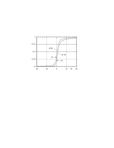
FIGURE 6.: The functions $R^{\prime}/R$ and $R^{\prime\prime}/R$.

a. Alternative expressions for the coefficients $C_{i}$.

The coefficients $C_{i}$ can also be written in terms of the Kummer function $M(a,c\,;x)$. First, on using the integral representation (A.5) for $M(a,c\,;x)$, the integral occurring in the expression (2.31) can be written as

$$\int_{0}^{1}\!\!{\rm d}{z}\,z^{2i}(1-z^{2})^{k}e^{\sigma z^{2}}=\frac{\Gamma(i+{\textstyle\frac{1}{2}})\Gamma(k+1)}{2\Gamma(i+k+\frac{3}{2})}M(i+{\textstyle\frac{1}{2}},i+k+{\textstyle\frac{3}{2}};\sigma)\;,$$ (2.37)

where $\Gamma(z)$ is the gamma (factorial) function [Eq. (A.2)]. If we introduce this expression into the expansion (2.31), we find the numerical coefficient

$$\frac{1}{(2i)!2^{2k}(k!)^{2}}\frac{\Gamma(i+{\textstyle\frac{1}{2}})\Gamma(k+1)}{2\Gamma(i+k+\frac{3}{2})}=\frac{1}{[2(i+k)+1]!}{i+k\choose k}\;,$$

where the basic property of the gamma function, $\Gamma(z+1)=z\Gamma(z)$, has been used. Then, on gathering the terms with the same power of $\xi$ in the resulting ${\cal Z}$ by dint of Eq. (2.34), we get

$${\cal Z}=2\sum_{i=0}^{\infty}\frac{\xi^{2i}}{(2i+1)!}\left\{\sum_{k=0}^{i}d_{i-k,k}(\alpha)M(i-k+{\textstyle\frac{1}{2}},i+{\textstyle\frac{3}{2}};\sigma)\right\}\;,$$

where the angular coefficients $d_{i,k}(\alpha)$ are given by

$$d_{i,k}(\alpha)={i+k\choose k}\cos^{2i}\!\alpha\sin^{2k}\!\alpha\;.$$ (2.38)

Consequently, on comparing with Eq. (2.35), we can finally express the coefficients $C_{i}$ as

$$C_{i}(\sigma,\alpha)=\frac{i!}{(2i+1)!}\sum_{k=0}^{i}d_{i-k,k}(\alpha)\frac{M(i-k+{\textstyle\frac{1}{2}},i+{\textstyle\frac{3}{2}};\sigma)}{M({\textstyle\frac{1}{2}},{\textstyle\frac{3}{2}};\sigma)}\;,$$ (2.39)

where we have used (see Appendix A)

$$R(\sigma)=M({\textstyle\frac{1}{2}},{\textstyle\frac{3}{2}};\sigma)\;.$$ (2.40)

Let us finally write in full the first few coefficients for future reference. If we introduce the first few angular coefficients $d_{i,k}(\alpha)$

$$\begin{array}[]{rclrclrcl}d_{0,0}&=&1\;,&d_{1,0}&=&\cos^{2}\!\alpha\;,&d_{0,1}&=&\sin^{2}\!\alpha\;,\\ d_{2,0}&=&\cos^{4}\!\alpha\;,&d_{1,1}&=&2\cos^{2}\!\alpha\sin^{2}\!\alpha\;,&d_{0,2}&=&\sin^{4}\!\alpha\;,\end{array}$$

into Eq. (2.39), we get:

$$C_{1}=\frac{1}{3!}\left[\frac{M({\textstyle\frac{3}{2}},{\textstyle\frac{5}{2}};\sigma)}{M({\textstyle\frac{1}{2}},{\textstyle\frac{3}{2}};\sigma)}\cos^{2}\!\alpha+\frac{M({\textstyle\frac{1}{2}},{\textstyle\frac{5}{2}};\sigma)}{M({\textstyle\frac{1}{2}},{\textstyle\frac{3}{2}};\sigma)}\sin^{2}\!\alpha\right]\;,$$ (2.41)

and

$$C_{2}=\frac{1}{60}\left[\frac{M({\textstyle\frac{5}{2}},{\textstyle\frac{7}{2}};\sigma)}{M({\textstyle\frac{1}{2}},{\textstyle\frac{3}{2}};\sigma)}\cos^{4}\!\alpha+\frac{M({\textstyle\frac{3}{2}},{\textstyle\frac{7}{2}};\sigma)}{M({\textstyle\frac{1}{2}},{\textstyle\frac{3}{2}};\sigma)}2\cos^{2}\!\alpha\sin^{2}\!\alpha+\frac{M({\textstyle\frac{1}{2}},{\textstyle\frac{7}{2};\sigma)}}{M({\textstyle\frac{1}{2}},{\textstyle\frac{3}{2}};\sigma)}\sin^{4}\!\alpha\right]\;.$$

The coefficients $C_{i}$ can also be expressed in terms of the averages of $\vec{m}$ in zero field. To this end, let us begin from the definition of the partition function

$${\cal Z}=\int\!\!{\rm d}{\Omega}\,\exp[\sigma(\vec{e}\cdot\hat{n})^{2}+\xi(\vec{e}\cdot\hat{b})]\;,$$

where $\int\!{\rm d}{\Omega}\,(\cdot)=(1/2\pi)\int_{-1}^{1}\!{\rm d}{(\cos\vartheta)}\,\int_{0}^{2\pi}\!{\rm d}{\varphi}\,(\cdot)$ and the expression (2.4) for $-\beta{\cal H}$ have been used. Next, on expanding $\exp[\xi(\vec{e}\cdot\hat{b})]$ in powers of $\xi$, we obtain

$${\cal Z}=\sum_{i=0}^{\infty}\frac{\xi^{2i}}{(2i)!}\int\!\!{\rm d}{\Omega}\,(\vec{e}\cdot\hat{b})^{2i}\exp[\sigma(\vec{e}\cdot\hat{n})^{2}]$$

where to eliminate the odd powers of $\xi$ we have merely considered that $(\vec{e}\cdot\hat{b})^{2i+1}$ reverses its sign when the transformation $\vec{e}\to-\vec{e}$ is applied, whereas the term $\exp[\sigma(\vec{e}\cdot\hat{n})^{2}]$ is invariant against such transformation, whence $\int\!{\rm d}{\Omega}\,(\vec{e}\cdot\hat{b})^{2i+1}\exp[\sigma(\vec{e}\cdot\hat{n})^{2}]\equiv 0$. Finally, on comparing the above expansion of ${\cal Z}$ with ${\cal Z}=2R\sum_{i=0}^{\infty}(C_{i}/i!)\xi^{2i}$, noting that $R(\sigma)$ can be written as $R(\sigma)=(1/2)\int\!{\rm d}{\Omega}\,\exp[\sigma(\vec{e}\cdot\hat{n})^{2}]$, and introducing the thermal-equilibrium averages in zero field [cf. Eq. (2.10)]

$$\left.\big{\langle}(\vec{e}\cdot\hat{b})^{n}\big{\rangle}_{{\rm e}}\right|_{B=0}=\frac{\int\!{\rm d}{\Omega}\,(\vec{e}\cdot\hat{b})^{n}\exp[\sigma(\vec{e}\cdot\hat{n})^{2}]}{\int\!{\rm d}{\Omega}\,\exp[\sigma(\vec{e}\cdot\hat{n})^{2}]}\;,$$

we arrive at the desired relation

$$\frac{C_{i}(\sigma,\alpha)}{i!}=\frac{1}{(2i)!}\left.\big{\langle}(\vec{e}\cdot\hat{b})^{2i}\big{\rangle}_{{\rm e}}\right|_{B=0}\;.$$ (2.42)

b. Particular cases of the coefficients $C_{i}$.

Let us briefly consider the form that the coefficients appearing in the field expansion of the partition function take in the particular cases considered in Subsec. II.C. To this end, the alternative expression for those coefficients in terms of Kummer functions [Eq. (2.39)] results to be more convenient.

1. On noting that $M(a,c\,;x=0)=1$ [see the definition (A.1)], one gets for $C_{i}$ in the isotropic case

   $$\frac{1}{i!}\left.C_{i}\right|_{\sigma=0}=\frac{1}{(2i+1)!}\sum_{k=0}^{i}{i\choose k}\cos^{2(i-k)}\!\alpha\sin^{2k}\!\alpha=\frac{1}{(2i+1)!}\;,$$

   since the sum is equal to $(\cos^{2}\!\alpha+\sin^{2}\!\alpha)^{i}=1$.

2. In the $\sigma\to\infty$ limit, on employing the asymptotic expansion (A.16) of $M(a,c\,;x)$ for large positive argument, one finds

   $$\left.\frac{M(i-k+{\textstyle\frac{1}{2}},i+{\textstyle\frac{3}{2}};\sigma)}{M({\textstyle\frac{1}{2}},{\textstyle\frac{3}{2}};\sigma)}\right|_{\sigma\gg 1}=\frac{\Gamma(i+\frac{3}{2})}{\Gamma(i-k+{\textstyle\frac{1}{2}})}\frac{2}{\sigma^{k}}\stackrel{{\scriptstyle\sigma\to\infty}}{{\longrightarrow}}(2i+1)\delta_{k,0}\;,$$

   where we have used $\Gamma(i+3/2)=(i+1/2)\Gamma(i+1/2)$. Therefore, the general expression (2.39) reduces in the Ising case to

   $$\frac{1}{i!}\left.C_{i}\right|_{\sigma\to\infty}=\frac{\cos^{2i}\!\alpha}{(2i)!}\;.$$

3. To get the $\sigma\to-\infty$ limit of $C_{i}$, we can now use the asymptotic expansion (c) of $M(a,c\,;x)$ for large negative argument. On doing so, one first finds

   $$\left.\frac{M(i-k+{\textstyle\frac{1}{2}},i+{\textstyle\frac{3}{2}};\sigma)}{M({\textstyle\frac{1}{2}},{\textstyle\frac{3}{2}};\sigma)}\right|_{\sigma\ll-1}=\frac{\Gamma(i+\frac{3}{2})}{{\textstyle\frac{1}{2}}\pi^{1/2}k!}\frac{1}{(-\sigma)^{i-k}}\stackrel{{\scriptstyle\sigma\to-\infty}}{{\longrightarrow}}\frac{2\Gamma(i+\frac{3}{2})}{\pi^{1/2}i!}\delta_{i,k}\;.$$

   Therefore, by using Eq. (A.21) for the gamma function of half-odd-integer argument, the plane-rotator $C_{i}$ reads

   $$\frac{1}{i!}\left.C_{i}\right|_{\sigma\to-\infty}=\left(\frac{\sin\alpha}{2}\right)^{2i}\frac{1}{(i!)^{2}}\;.$$

4. The longitudinal-field case corresponds to set $\alpha=0$ in the expression (2.39) for $C_{i}(\sigma,\alpha)$. On doing this and using $d_{i-k,k}|_{\alpha=0}=\delta_{k,0}$ [see Eq. (2.38)], one gets

   $$\frac{1}{i!}\left.C_{i}\right|_{\alpha=0}=\frac{1}{(2i+1)!}\frac{M(i+{\textstyle\frac{1}{2}},i+{\textstyle\frac{3}{2}};\sigma)}{M({\textstyle\frac{1}{2}},{\textstyle\frac{3}{2}};\sigma)}=\frac{1}{(2i)!}\frac{R^{(i)}(\sigma)}{R(\sigma)}$$

   where the relations (A.3) between the functions $R^{(\ell)}$ and Kummer functions have been taken into account.

All these particular cases of the coefficients $C_{i}$ are summarized in Table III, while the first few ones are displayed in Table IV.

TABLE III.: Expressions for the coefficients $C_{i}/i!$ of the field expansion of the partition function in the isotropic, Ising, plane-rotator, and longitudinal-field cases.

	$\sigma=0$	$\sigma\to\infty$	$\sigma\to-\infty$	$\vec{B}\parallel\hat{n}$
${\displaystyle\frac{C_{i}}{i!}}$	${\displaystyle\frac{1}{(2i+1)!}}$	${\displaystyle\frac{\cos^{2i}\!\alpha}{(2i)!}}$	${\displaystyle\frac{\sin^{2i}\!\alpha}{2^{2i}(i!)^{2}}}$	${\displaystyle\frac{1}{(2i)!}\frac{R^{(i)}}{R}}$

TABLE IV.: The coefficients $C_{1}$, $C_{2}$, and $C_{3}$ in the isotropic, Ising, plane-rotator, and longitudinal-field cases.

	$\sigma=0$	$\sigma\to\infty$	$\sigma\to-\infty$	$\vec{B}\parallel\hat{n}$
$C_{1}$	${\displaystyle\frac{1}{6}}$	${\displaystyle\frac{1}{2}\cos^{2}\!\alpha}$	${\displaystyle\frac{1}{4}\sin^{2}\!\alpha}$	${\displaystyle\frac{1}{2}\frac{R^{\prime}}{R}}$
$C_{2}$	${\displaystyle\frac{1}{60}}$	${\displaystyle\frac{1}{12}\cos^{4}\!\alpha}$	${\displaystyle\frac{1}{32}\sin^{4}\!\alpha}$	${\displaystyle\frac{1}{12}\frac{R^{\prime\prime}}{R}}$
$C_{3}$	${\displaystyle\frac{1}{840}}$	${\displaystyle\frac{1}{120}\cos^{6}\!\alpha}$	${\displaystyle\frac{1}{384}\sin^{6}\!\alpha}$	${\displaystyle\frac{1}{120}\frac{R^{\prime\prime\prime}}{R}}$

2. Expansion of the partition function in powers of the anisotropy parameter

We shall now derive the first few terms in the expansion of ${\cal Z}$ in powers of $\sigma=Kv/k_{{\rm B}}T$. This expansion will be a suitable description of the thermodynamical properties when the anisotropy energy is sufficiently small in comparison with the thermal energy.

In order to perform this expansion, it is more convenient to rotate the spherical coordinate system to set the polar axis pointing along the external field $\vec{B}$ (see Fig. 2; the anisotropy axis $\hat{n}$ is now in the $xz$-plane and $\alpha$ is its polar angle). With this choice of coordinates, the partition function reads

$${\cal Z}=\frac{1}{2\pi}\int_{0}^{\pi}\!\!{\rm d}{\vartheta}\,\sin\vartheta\exp(\xi\cos\vartheta)\int_{0}^{2\pi}\!\!{\rm d}{\varphi}\,\exp[\sigma(\cos\alpha\cos\vartheta+\sin\alpha\sin\vartheta\cos\varphi)^{2}]\;.$$

If we now expand the second exponential, we get an expression of the form

$${\cal Z}=\sum_{i=0}^{\infty}\frac{\sigma^{i}}{i!}{\cal Z}_{i}\;,$$ (2.43)

where

$${\cal Z}_{i}=\frac{1}{2\pi}\int_{0}^{\pi}\!\!{\rm d}{\vartheta}\,\sin\vartheta\exp(\xi\cos\vartheta)\int_{0}^{2\pi}\!\!{\rm d}{\varphi}\,(\cos\alpha\cos\vartheta+\sin\alpha\sin\vartheta\cos\varphi)^{2i}\;.$$ (2.44)

Note that the zeroth order coefficient is naturally the isotropic partition function ${\cal Z}_{0}=(2/\xi)\sinh\xi$ [Eq. (2.17)].

On using the binomial expansion in the second integrand of Eq. (2.44), and employing the following result (Arfken, 1985, p. 318),

$$\frac{1}{2\pi}\int_{0}^{2\pi}\!\!{\rm d}{\varphi}\,\cos^{n}\!\varphi=\left\{\begin{array}[]{cl}0&\mbox{for~{}odd~{}}n\\ {\displaystyle\frac{(2k)!}{2^{2k}(k!)^{2}}}&\mbox{ for }n=2k\end{array}\;,\right.$$ (2.45)

to do the integrals over the azimuthal angle, we see that only even powers of $\cos\alpha$ and $\sin\alpha$ appear in ${\cal Z}_{i}$. On the other hand, $\sin^{2k}\!\vartheta$ can always be expressed as a sum of powers of the form $\cos^{2\ell}\!\vartheta$, with $\ell\leq k$, namely

$$\sin^{2k}\!\vartheta=(1-\cos^{2}\!\vartheta)^{k}=\sum_{\ell=0}^{k}{k\choose\ell}(-1)^{\ell}\cos^{2\ell}\!\vartheta\;.$$

Accordingly, on introducing once more the substitution $z=\cos\vartheta$ and noting that,

$$\int_{-1}^{1}\!\!{\rm d}{z}\,z^{n}\exp(\xi z)=\frac{{\rm d}^{n}{}}{{\rm d}\xi^{n}}\int_{-1}^{1}\!\!{\rm d}{z}\,\exp(\xi z)=\frac{{\rm d}^{n}{}}{{\rm d}\xi^{n}}{\cal Z}_{0}\;,$$ (2.46)

one realizes that all the functions ${\cal Z}_{i}$ can be expressed in terms of the isotropic partition function, ${\cal Z}_{0}$, and its $\xi$-derivatives. For instance, ${\cal Z}_{1}$ reads

$${\cal Z}_{1} = \cos^{2}\!\alpha\int_{-1}^{1}\!\!{\rm d}{z}\,z^{2}\exp(\xi z)+\frac{1}{2}\sin^{2}\!\alpha\int_{-1}^{1}\!\!{\rm d}{z}\,(1-z^{2})\exp(\xi z)$$ (2.47)

$$= {\cal Z}^{\prime\prime}_{0}\cos^{2}\!\alpha+\frac{1}{2}({\cal Z}_{0}-{\cal Z}^{\prime\prime}_{0})\sin^{2}\!\alpha\;,$$

where the prime denotes differentiation with respect to $\xi$. On the other hand, since ${\cal Z}_{0}=(2/\xi)\sinh\xi$, the derivative ${\cal Z}^{\prime}_{0}$ is given by

$${\cal Z}^{\prime}_{0}=L(\xi){\cal Z}_{0}\;,$$ (2.48)

where

$$L(\xi)=\coth\xi-\frac{1}{\xi}\;,$$ (2.49)

is the celebrated Langevin function. On taking a further $\xi$-derivative and using the relation between $L^{\prime}$ and $L$, namely

$$L^{\prime}=1-\frac{2}{\xi}L-L^{2}\;,$$ (2.50)

we get for the combinations of ${\cal Z}_{0}$ and ${\cal Z}^{\prime\prime}_{0}$ occurring in Eq. (2.47)

$${\cal Z}^{\prime\prime}_{0}={\cal Z}_{0}\left(1-\frac{2}{\xi}L\right)\;,\qquad\frac{1}{2}({\cal Z}_{0}-{\cal Z}^{\prime\prime}_{0})={\cal Z}_{0}\frac{1}{\xi}L\;.$$ (2.51)

Therefore, on introducing these results in Eq. (2.47), we finally get

$$\frac{{\cal Z}_{1}}{{\cal Z}_{0}}=\left(1-\frac{2}{\xi}L\right)\cos^{2}\!\alpha+\frac{1}{\xi}L\sin^{2}\!\alpha\;.$$ (2.52)

The calculation of ${\cal Z}_{2}$ proceeds similarly. On taking the definition (2.44) into account and using $z=\cos\vartheta$, one obtains

$${\cal Z}_{2} = \cos^{4}\!\alpha\int_{-1}^{1}\!\!{\rm d}{z}\,z^{4}e^{\xi z}+\frac{6}{2}\cos^{2}\!\alpha\sin^{2}\!\alpha\int_{-1}^{1}\!\!{\rm d}{z}\,z^{2}(1-z^{2})e^{\xi z}$$

$${}+\frac{3}{8}\sin^{4}\!\alpha\int_{-1}^{1}\!\!{\rm d}{z}\,(1-z^{2})^{2}e^{\xi z}\;,$$

where Eq. (2.45) has been used for calculating the integrals over $\varphi$. Consequently, in terms of ${\cal Z}_{0}$ and its derivatives, ${\cal Z}_{2}$ is given by

$${\cal Z}_{2}={\cal Z}^{\prime\prime\prime\prime}_{0}\cos^{4}\!\alpha+3({\cal Z}^{\prime\prime}_{0}-{\cal Z}^{\prime\prime\prime\prime}_{0})\cos^{2}\!\alpha\sin^{2}\!\alpha+\frac{3}{8}({\cal Z}_{0}-2{\cal Z}^{\prime\prime}_{0}+{\cal Z}^{\prime\prime\prime\prime}_{0})\sin^{4}\!\alpha\;.$$ (2.53)

In order to take the 4th-order derivative ${\cal Z}^{\prime\prime\prime\prime}_{0}$, one can repeatedly use Eqs. (2.48) and (2.50). However, it significantly simplifies the calculations to obtain first the derivative $(L/\xi)^{\prime}$, which can be written as

$$\left(\frac{1}{\xi}L\right)^{\prime}=-\frac{1}{\xi}\left[L^{2}-\left(1-\frac{3}{\xi}L\right)\right]\;.$$ (2.54)

Thus, after some manipulation, one gets the expression

$${\cal Z}^{\prime\prime\prime\prime}_{0}={\cal Z}_{0}\left[1-\frac{4}{\xi}L+\frac{8}{\xi^{2}}\left(1-\frac{3}{\xi}L\right)\right]\;,$$

which, along with Eqs. (2.51), gives

$${\cal Z}^{\prime\prime\prime\prime}_{0}-{\cal Z}^{\prime\prime}_{0}=2{\cal Z}_{0}\left[\frac{4}{\xi^{2}}\left(1-\frac{3}{\xi}L\right)-\frac{1}{\xi}L\right]\;,\quad{\cal Z}_{0}-2{\cal Z}^{\prime\prime}_{0}+{\cal Z}^{\prime\prime\prime\prime}_{0}={\cal Z}_{0}\frac{8}{\xi^{2}}\left(1-\frac{3}{\xi}L\right)\;.$$

On introducing all these results into Eq. (2.53), we finally find for ${\cal Z}_{2}$:

$$\frac{{\cal Z}_{2}}{{\cal Z}_{0}} = \left[1-\frac{4}{\xi}L+\frac{8}{\xi^{2}}\left(1-\frac{3}{\xi}L\right)\right]\cos^{4}\!\alpha$$ (2.55)

$${}+6\left[\frac{1}{\xi}L-\frac{4}{\xi^{2}}\left(1-\frac{3}{\xi}L\right)\right]\cos^{2}\!\alpha\sin^{2}\!\alpha+\left[\frac{3}{\xi^{2}}\left(1-\frac{3}{\xi}L\right)\right]\sin^{4}\!\alpha\;.\qquad\quad$$

This formula completes the explicit expansion of the partition function in powers of the anisotropy parameter up to second order.

3. Asymptotic expansion of the partition function for strong anisotropy

In order to complement the above derived weak-anisotropy expansion, we shall now carry out an asymptotic expansion of the partition function for strong anisotropy (easy-axis case only). As will be seen below, the approximate thermal-equilibrium quantities obtained from the combined use of those expansions, well approximate the exact results in the whole temperature range. Therefore we shall be able to get simple analytical expressions for the thermodynamical quantities that reasonably avoid the necessity of their computation by numerical methods.

In order to perform an expansion of the partition function for large $\sigma=Kv/k_{{\rm B}}T$, we shall start from the field expansion (2.35) of ${\cal Z}$ and use the asymptotic results for its coefficients. Then, we shall obtain a number of infinite series of powers of $\xi=mB/k_{{\rm B}}T$, which will be identified as certain elementary functions, obtaining in this way a closed asymptotic expression for ${\cal Z}$.

We start by recalling that the whole coefficient of $\xi^{2i}$ in the general $\xi$-expansion of ${\cal Z}$ reads [see Eqs. (2.35) and (2.39)]

$$\frac{2R(\sigma)C_{i}}{i!}=\frac{2}{(2i+1)!}\sum_{k=0}^{i}d_{i-k,k}(\alpha)M(i-k+{\textstyle\frac{1}{2}},i+{\textstyle\frac{3}{2}};\sigma)\;,$$ (2.56)

where $R(\sigma)=M({\textstyle\frac{1}{2}},{\textstyle\frac{3}{2}};\sigma)$ has been used [Eq. (2.40)], and $d_{i-k,k}(\alpha)$ is explicitly given by [see Eq. (2.38)]

$$d_{i-k,k}(\alpha)={i\choose k}\cos^{2(i-k)}\!\alpha\sin^{2k}\!\alpha\;.$$ (2.57)

On the other hand, the asymptotic expansion (A.16) of the confluent hypergeometric functions yields for $\sigma\gg 1$

$$M(i-k+{\textstyle\frac{1}{2}},i+{\textstyle\frac{3}{2}};\sigma) = \frac{e^{\sigma}}{2\sigma}\frac{2\Gamma(i+{\textstyle\frac{3}{2}})}{\Gamma(i-k+{\textstyle\frac{1}{2}})}\frac{1}{\sigma^{k}}\bigg{[}1+\frac{(2k-2i+1)(k+1)}{2\sigma}$$

$${}+\frac{(2k-2i+3)(2k-2i+1)(k+1)(k+2)}{8\sigma^{2}}+\cdots\bigg{]}\;.$$

Considering that the sum in Eq. (2.56), begins at $k=0$, and that we shall carry out the expansion of ${\cal Z}$ through order $1/\sigma^{2}$, we write

$$\sum_{k=0}^{i}d_{i-k,k}M(i-k+{\textstyle\frac{1}{2}},i+{\textstyle\frac{3}{2}};\sigma)\simeq\cos^{2i}\!\alpha\,M(i+{\textstyle\frac{1}{2}},i+{\textstyle\frac{3}{2}};\sigma)$$

$${}+\frac{1}{2}(2i)\cos^{2(i-1)}\!\alpha\sin^{2}\!\alpha\,M(i-{\textstyle\frac{1}{2}},i+{\textstyle\frac{3}{2}};\sigma)$$

$${}+\frac{1}{8}(2i)(2i-2)\cos^{2(i-2)}\!\alpha\sin^{4}\!\alpha\,M(i-{\textstyle\frac{3}{2}},i+{\textstyle\frac{3}{2}};\sigma)\;,$$

where we have taken Eq. (2.57) into account. Now, on using $\Gamma(z+1)=z\Gamma(z)$, we get for the quotients of gamma functions occurring in the above equation via the Kummer functions

$$\frac{2\Gamma(i+{\textstyle\frac{3}{2}})}{\Gamma(i-k+{\textstyle\frac{1}{2}})}=\left\{\begin{array}[]{cl}\;\;\;(2i+1),&\mbox{ for }k=0\\ {\textstyle\frac{1}{2}}(2i+1)(2i-1),&\mbox{ for }k=1\\ \frac{1}{4}(2i+1)(2i-1)(2i-3),&\mbox{ for }k=2\end{array}\right.\;.$$

On collecting all these intermediate results, we can approximately write the $i$th term in the $\xi$-expansion of ${\cal Z}$ in the form

$$\frac{\sigma}{e^{\sigma}}\frac{2R(\sigma)C_{i}}{i!}\;\xi^{2i} \simeq \frac{\xi_{\|}^{2i}}{(2i)!}\left[1-\frac{(2i-1)}{2\sigma}+\frac{(2i-1)(2i-3)}{4\sigma^{2}}\right]$$

$${}+\frac{\xi_{\|}^{2(i-1)}\xi_{\perp}^{2}}{[2(i-1)]!}\left[\frac{1}{4\sigma}-\frac{(2i-3)}{4\sigma^{2}}\right]+\frac{\xi_{\|}^{2(i-2)}\xi_{\perp}^{4}}{[2(i-2)]!}\frac{1}{32\sigma^{2}}\;,$$

where we have multiplied across by $\sigma/e^{\sigma}$ to avoid writing $e^{\sigma}/\sigma$ in all the right-hand sides of the subsequent equations. In addition, in the above equation we have introduced the longitudinal and transverse components of the dimensionless field: $\xi_{\|}=\xi\cos\alpha$ and $\xi_{\perp}=\xi\sin\alpha$. Note however that Eq. (3.) only holds for the terms with $i\geq 2$. For $i=1$, the sum in $k$ in the expression (2.39) only runs over $k=0$ and $k=1$; therefore, the last term on the right-hand side of Eq. (3.) is absent. Similarly, for $i=0$, only the first term remains. Taking these considerations into account by properly adjusting the summation limits in the following expression, we can already write down the partition function ${\cal Z}=2R\sum_{i=0}^{\infty}(C_{i}/i!)\xi^{2i}$ as

$$\frac{\sigma}{e^{\sigma}}{\cal Z} \simeq \sum_{i=0}^{\infty}\frac{\xi_{\|}^{2i}}{(2i)!}\left[1-\frac{(2i-1)}{2\sigma}+\frac{(2i-1)(2i-3)}{4\sigma^{2}}\right]$$

$${}+\frac{1}{4\sigma}\sum_{i=1}^{\infty}\frac{\xi_{\|}^{2(i-1)}\xi_{\perp}^{2}}{[2(i-1)]!}\left[1-\frac{(2i-3)}{\sigma}\right]+\frac{1}{32\sigma^{2}}\sum_{i=2}^{\infty}\frac{\xi_{\|}^{2(i-2)}\xi_{\perp}^{4}}{[2(i-2)]!}\;.$$

If we now redefine the summation indices in order to force all the above series to start at the value zero of the corresponding new index and gather the terms multiplying the same type of series, we get

$$\frac{\sigma}{e^{\sigma}}{\cal Z} \simeq \left(1+\frac{1}{4\sigma}\xi_{\perp}^{2}+\frac{1}{32\sigma^{2}}\xi_{\perp}^{4}\right)\sum_{i=0}^{\infty}\frac{\xi_{\|}^{2i}}{(2i)!}$$

$${}-\left(\frac{1}{2\sigma}+\frac{1}{4\sigma^{2}}\xi_{\perp}^{2}\right)\sum_{i=0}^{\infty}\frac{\xi_{\|}^{2i}}{(2i)!}(2i-1)+\frac{1}{4\sigma^{2}}\sum_{i=0}^{\infty}\frac{\xi_{\|}^{2i}}{(2i)!}(2i-1)(2i-3)\;.$$

Our last goal is to identify all the power series occurring in Eq. (3.). The series in the first term on the right-hand side is precisely that of the hyperbolic cosine, $\cosh x=\sum_{i=0}^{\infty}x^{2i}/(2i)!$. The other two series can also be identified after some redefinition of the summation indices ($k=i-1$):

$$\sum_{i=0}^{\infty}\frac{x^{2i}}{(2i)!}(2i-1)=\sum_{k=0}^{\infty}\frac{x^{2k+2}}{(2k+1)!}-\cosh x=x\sinh x-\cosh x\;,$$

while

$$\sum_{i=0}^{\infty}\frac{x^{2i}}{(2i)!}(2i-1)(2i-3) = \sum_{k=0}^{\infty}\frac{x^{2(k+1)}}{(2k)!}-3(x\sinh x-\cosh x)$$

$$= (x^{2}+3)\cosh x-3x\sinh x\;.$$

Finally, we insert these results into Eq. (3.), gather the terms with the same power of $1/\sigma$, and extract a factor $\cosh\xi_{\|}$, obtaining

$${\cal Z}\simeq\frac{e^{\sigma}}{\sigma}\cosh\xi_{\|} \bigg{\{} 1+\frac{1}{4\sigma}\left[(2+\xi_{\perp}^{2})-2\xi_{\|}\tanh\xi_{\|}\right]$$

$${}+\frac{1}{4\sigma^{2}}\left[\left(3+\xi_{\|}^{2}+\xi_{\perp}^{2}+\frac{1}{8}\xi_{\perp}^{4}\right)-(3+\xi_{\perp}^{2})\xi_{\|}\tanh\xi_{\|}\right]\bigg{\}}\;.$$

This equation is the desired asymptotic expansion of the partition function. Note that, as could be expected, the leading term in this equation is precisely what we called partition function in the Ising regime [Eq. (2.22)].

II.E Series expansions of the free energy

Once one has obtained an expansion of the partition function in a series of powers of a given quantity, one needs to construct the corresponding expansion of $\ln{\cal Z}$ in order to obtain the relevant thermal-equilibrium quantities (see Table II). Here, we shall derive the expansions of the free energy ${\cal F}=-k_{{\rm B}}T\ln{\cal Z}$ corresponding to those developed above for the partition function.

1. Expansion of the logarithm of a function

The problem of constructing the series expansion of the logarithm of a function with a given series representation appears in a number of physical and mathematical problems (e.g., in the construction of the cumulants of a probability distribution in terms of the known moments of such distribution; see Risken, 1989). Thus, if one has derived an expansion of the partition function of the type

$${\cal Z}(y)={\cal Z}(0)\sum_{i=0}^{\infty}\frac{A_{i}}{i!}y^{i}\;,$$ (2.61)

(note that $A_{0}=1$), the first few terms in the corresponding expansion of $\ln{\cal Z}$ are given by

$$\ln{\cal Z}(y) = \ln{\cal Z}(0)+A_{1}y+\frac{1}{2}\left(A_{2}-A_{1}^{2}\right)y^{2}+\frac{1}{6}\left(A_{3}-3A_{2}A_{1}+2A_{1}^{3}\right)y^{3}$$ (2.62)

$${}+\frac{1}{24}\left(A_{4}-4A_{3}A_{1}-3A_{2}^{2}+12A_{2}A_{1}^{2}-6A_{1}^{4}\right)y^{4}+\cdots\;.$$

This formula, when multiplied by $-k_{{\rm B}}T$, gives the first few terms of the $y$-expansion of the free energy.

2. Averages for anisotropy axes distributed at random

In what follows we shall frequently consider the values of the relevant quantities for an ensemble of magnetic moments whose anisotropy axes are distributed at random. Note that averaging, in the sense of keep fixed some parameters and then sum over the remainder ones (e.g., anisotropy-axis orientations), does not make sense for the partition function since, for independent entities, ${\cal Z}$ is a multiplicative quantity. On the other hand, averaging makes sense for the customary thermodynamical functions (free energy, entropy, energy, etc.) as they are additive quantities.

When averaging the thermodynamical quantities over assemblies of equivalent magnetic moments (i.e., with the same characteristic parameters) whose anisotropy axes are distributed at random, we shall need to calculate integrals of the general form

$$\left\langle f(\varphi_{\hat{n}},\alpha)\right\rangle_{{\rm ran}}=\frac{1}{4\pi}\int_{0}^{2\pi}\!\!{\rm d}{\varphi_{\hat{n}}}\,\int_{0}^{\pi}\!\!{\rm d}{\alpha}\,\sin\alpha f(\varphi_{\hat{n}},\alpha)\;,$$

where $\varphi_{\hat{n}}$ and $\alpha$ are, respectively, the azimuthal and polar angles of the unit vector along the anisotropy axis $\hat{n}$. We shall be mainly interested in the cases where $f(\varphi_{\hat{n}},\alpha)=\cos^{2i}\!\alpha\sin^{2k}\!\alpha$, which does not depend on the azimuthal angle. For these functions, one finds

$$\left\langle\cos^{2i}\!\alpha\sin^{2k}\!\alpha\right\rangle_{{\rm ran}}=\frac{1}{2}\int_{0}^{\pi}\!\!{\rm d}{\alpha}\,\sin\alpha\cos^{2i}\!\alpha\sin^{2k}\!\alpha\stackrel{{\scriptstyle x=\cos\alpha}}{{=}}\int_{0}^{1}\!\!{\rm d}{x}\,x^{2i}(1-x^{2})^{k}\;.$$

Now, on comparing with the relation (2.37) between integrals of $z^{2i}(1-z^{2})^{k}$ weighted by $\exp(\sigma z^{2})$, and Kummer functions, we get the expression

$$\left\langle\cos^{2i}\!\alpha\sin^{2k}\!\alpha\right\rangle_{{\rm ran}}=\frac{\Gamma(i+{\textstyle\frac{1}{2}})k!}{2\Gamma(i+k+{\textstyle\frac{3}{2}})}\;,$$ (2.63)

where we have employed $M(a,c\,;x=0)=1$ [see Eq. (A.1)] and $\Gamma(k+1)=k!$. Alternatively, on using $\Gamma(z+1)=z\Gamma(z)$ to expand the above quotient of gamma functions, we obtain

$$\left\langle\cos^{2i}\!\alpha\sin^{2k}\!\alpha\right\rangle_{{\rm ran}}=\frac{2^{k}\;k!}{\underbrace{(2i+1)[(2i+1)+2]\cdots[(2i+1)+2k]}_{k+1\;{\rm terms}}}\;.$$

To conclude, we explicitly write down the particular cases of the above results that, in what follows, will more frequently be used:

$$\begin{array}[]{rclrclrcl}\langle\cos^{2}\!\alpha\rangle_{{\rm ran}}&=&1/3\;,&\langle\sin^{2}\!\alpha\rangle_{{\rm ran}}&=&2/3\;,&&{}\hfil&\\ \left\langle\cos^{4}\!\alpha\right\rangle_{{\rm ran}}&=&1/5\;,&\left\langle\cos^{2}\!\alpha\sin^{2}\!\alpha\right\rangle_{{\rm ran}}&=&2/15\;,&\left\langle\sin^{4}\!\alpha\right\rangle_{{\rm ran}}&=&8/15\;.\end{array}$$ (2.64)

3. Field expansion of the free energy

On considering the expansion (2.35) of the partition function in powers of $\xi=mB/k_{{\rm B}}T$, one realizes that the function $2R(\sigma)$, $\xi^{2}$, and $C_{i}$ play the rôle, respectively, of ${\cal Z}(0)$, $y$, and $A_{i}$ in the generic $y$-expansion (2.61). Consequently, the corresponding general series (2.62) for $\ln{\cal Z}$ yields in this case

$$\ln{\cal Z}=\ln[2R(\sigma)]+C_{1}(\sigma,\alpha)\xi^{2}+\frac{1}{2}\left[C_{2}(\sigma,\alpha)-C_{1}(\sigma,\alpha)^{2}\right]\xi^{4}+\cdots\;.$$ (2.65)

This result shows the convenience of the introduction of the factor $i!$ in the definition (2.36) of the coefficients $C_{i}$: the general expansion (2.62) can then be directly used by merely replacing the coefficients $A_{i}$ by the $C_{i}$ ones.

Now, on introducing the first few angular terms $b_{i,k}(\alpha)$ [Eq. (2.30)],

$$\begin{array}[]{rclrclrcl}b_{0,0}&=&1\;,&b_{1,0}&=&{\textstyle\frac{1}{2}}\cos^{2}\!\alpha\;,&b_{0,1}&=&\frac{1}{4}\sin^{2}\!\alpha\;,\\ b_{2,0}&=&\frac{1}{24}\cos^{4}\!\alpha\;,&b_{1,1}&=&\frac{1}{8}\cos^{2}\!\alpha\sin^{2}\!\alpha\;,&b_{0,2}&=&\frac{1}{64}\sin^{4}\!\alpha\;,\end{array}$$

into the definition (2.36), one gets for the first coefficients $C_{i}$: $C_{0}=1$,

$$C_{1}=\frac{1}{2}\left(\frac{R^{\prime}}{R}\cos^{2}\!\alpha+\frac{R-R^{\prime}}{2R}\sin^{2}\!\alpha\right)\;,$$ (2.66)

and

$$C_{2}=\frac{1}{4}\left(\frac{1}{3}\frac{R^{\prime\prime}}{R}\cos^{4}\!\alpha+\frac{R^{\prime}-R^{\prime\prime}}{R}\cos^{2}\!\alpha\sin^{2}\!\alpha+\frac{R-2R^{\prime}+R^{\prime\prime}}{8R}\sin^{4}\!\alpha\right)\;,$$

where, instead of superscripts, we have used primes to indicate derivatives of $R(\sigma)$ with respect to its argument. On using these formulae we get for the coefficient of $\xi^{4}$ in the expansion (2.65),

$$\frac{1}{2}\left(C_{2}-C_{1}^{2}\right)=\frac{1}{8} \Bigg{\{} \left[\frac{1}{3}\frac{R^{\prime\prime}}{R}-\bigg{(}\frac{R^{\prime}}{R}\bigg{)}^{2}\right]\cos^{4}\!\alpha$$ (2.67)

$${}+\left[\bigg{(}\frac{R^{\prime}}{R}\bigg{)}^{2}-\frac{R^{\prime\prime}}{R}\right]\cos^{2}\!\alpha\sin^{2}\!\alpha$$

$${}+\frac{1}{8}\left[-1+2\frac{R^{\prime}}{R}-2\bigg{(}\frac{R^{\prime}}{R}\bigg{)}^{2}+\frac{R^{\prime\prime}}{R}\right]\sin^{4}\!\alpha\Bigg{\}}\;.$$

Equations (2.66) and (2.67), along with (2.65), yield the desired $\xi$-expansion of the free energy up to the fourth order.

In Section III we shall introduce the reduced linear and non-linear susceptibilities. These quantities, which incorporate the anisotropy-induced temperature dependence of the susceptibilities, are directly related with $C_{1}$ and $(C_{2}-C_{1}^{2})$, respectively.

Average for anisotropy axes distributed at random.

On introducing the values of the averaged trigonometric coefficients (2.64) into Eq. (2.66), we get $\left\langle C_{1}\right\rangle_{{\rm ran}}=1/6$. Proceeding similarly with the expression (2.67) for $(C_{2}-C_{1}^{2})/2$, one obtains

$$\frac{1}{2}\left\langle C_{2}-C_{1}^{2}\right\rangle_{{\rm ran}}=\frac{1}{120}\left[2\frac{R^{\prime}}{R}-3\bigg{(}\frac{R^{\prime}}{R}\bigg{)}^{2}-1\right]\;.$$ (2.68)

If we introduce these results into the $\xi$-expansion of $\ln{\cal Z}$ [Eq. (2.65)], we finally get for the free energy of an ensemble of equivalent dipoles with anisotropy axes distributed at random:

$$\left\langle{\cal F}\right\rangle_{{\rm ran}}=-k_{{\rm B}}T\left\{\ln[2R(\sigma)]+\frac{1}{6}\xi^{2}+\frac{1}{120}\left[2\frac{R^{\prime}}{R}-3\bigg{(}\frac{R^{\prime}}{R}\bigg{)}^{2}-1\right]\xi^{4}+\cdots\right\}\;.$$ (2.69)

It is to be noted that the first correction, $-k_{{\rm B}}T\xi^{2}/6$, to the unbiased free energy $-k_{{\rm B}}T\ln[2R(\sigma)]$, does not depend on the magnetic anisotropy. This will take its reflection in, for example, the independence of the linear susceptibility on the anisotropy energy for systems with axes distributed at random (see Subsec. III.D).

4. Expansion of the free energy in powers of the anisotropy parameter

The expansion of the free energy in powers of $\sigma=Kv/k_{{\rm B}}T$ can be obtained similarly. Let us first rewrite the expansion (2.43) of the partition function in powers of $\sigma$ as

$${\cal Z}={\cal Z}_{0}\left(1+\frac{{\cal Z}_{1}}{{\cal Z}_{0}}\sigma+\frac{1}{2}\frac{{\cal Z}_{2}}{{\cal Z}_{0}}\sigma^{2}+\cdots\right)\;,$$

where ${\cal Z}_{0}$ is a shorthand for ${\cal Z}_{{\rm Lan}}=(2/\xi)\sinh\xi$. If one compares this expansion with the general one (2.61), one sees that ${\cal Z}_{0}$, $\sigma$, and ${\cal Z}_{i}/{\cal Z}_{0}$ play the rôle, respectively, of ${\cal Z}(0)$, $y$, and $A_{i}$ there. Accordingly, we can immediately write down an equation similar to that obtained for the $\xi$-expansion of $\ln{\cal Z}$

$$\ln{\cal Z}\simeq{\ln{\cal Z}}_{{\rm Lan}}+\frac{{\cal Z}_{1}}{{\cal Z}_{0}}\;\sigma+\frac{1}{2}\left[\frac{{\cal Z}_{2}}{{\cal Z}_{0}}-\left(\frac{{\cal Z}_{1}}{{\cal Z}_{0}}\right)^{2}\right]\sigma^{2}\;.$$ (2.70)

Concerning the coefficients in this expansion, ${\cal Z}_{1}/{\cal Z}_{0}$ was already written in Eq. (2.52), namely

$$\frac{{\cal Z}_{1}}{{\cal Z}_{0}}=\left(1-\frac{2}{\xi}L\right)\cos^{2}\!\alpha+\frac{1}{\xi}L\sin^{2}\!\alpha\;,$$ (2.71)

while, taking Eq. (2.55) into account, one obtains after some algebra

$$\frac{1}{2}\left[\frac{{\cal Z}_{2}}{{\cal Z}_{0}}-\left(\frac{{\cal Z}_{1}}{{\cal Z}_{0}}\right)^{2}\right]=\frac{2}{\xi^{2}} \Bigg{\{} \left[2\left(1-\frac{3}{\xi}L\right)-L^{2}\right]\cos^{4}\!\alpha$$ (2.72)

$${}-\left[6\left(1-\frac{3}{\xi}L\right)-L^{2}-\xi L\right]\cos^{2}\!\alpha\sin^{2}\!\alpha$$

$${}+\frac{1}{4}\left[3\left(1-\frac{3}{\xi}L\right)-L^{2}\right]\sin^{4}\!\alpha\Bigg{\}}\;.$$

Equations (2.71) and (2.72), together with Eq. (2.70), yield the desired expansion of the free energy in powers of the anisotropy parameter up to second order.

Average for anisotropy axes distributed at random.

On introducing now the averages (2.64) of the trigonometric coefficients into the expression for ${\cal Z}_{1}/{\cal Z}_{0}$, one gets $\langle{\cal Z}_{1}/{\cal Z}_{0}\rangle_{{\rm ran}}=1/3$. Analogously, on averaging Eq. (2.72) one arrives at

$$\frac{1}{2}\left\langle\frac{{\cal Z}_{2}}{{\cal Z}_{0}}-\left(\frac{{\cal Z}_{1}}{{\cal Z}_{0}}\right)^{2}\right\rangle_{{\rm ran}}=\frac{2}{15}\left(2-\frac{3}{\xi}L\right)\frac{1}{\xi}L\;.$$

On introducing these results into the expansion (2.70) of $\ln{\cal Z}$, one gets for $\langle{\cal F}\rangle_{{\rm ran}}$ the approximate result

$$\left\langle{\cal F}\right\rangle_{{\rm ran}}=-k_{{\rm B}}T\left\{\ln\left(\frac{2}{\xi}\sinh\xi\right)+\frac{1}{3}\sigma+\frac{2}{15}\left[\left(2-\frac{3}{\xi}L\right)\frac{1}{\xi}L\right]\sigma^{2}+\cdots\right\}\;.$$ (2.73)

As $k_{{\rm B}}T\sigma=Kv$ [see Eqs. (2.3)] is a constant (neglecting the possible temperature dependence of $K$), we get the important result that, for anisotropy axes distributed at random, the corrections due to the magnetic anisotropy to the isotropic free energy, begin at order $\sigma^{2}$. This will lead to, for example, a dramatic decrease of the anisotropy effects on the magnetization curves for weakly anisotropic systems ($\sigma\,\raisebox{1.50696pt}{$<$}\raisebox{-2.79857pt}{$\sim$}\,2$) with a random distribution of anisotropy axes (see Subsec. III.C).

5. Asymptotic expansion of the free energy for strong anisotropy

Finally, the $1/\sigma$-expansion of the free energy can be obtained similarly. If we compare the asymptotic expansion (3.) for the partition function with the general one (2.61), we see that $(e^{\sigma}/\sigma)\cosh\xi_{\|}$ and $1/\sigma$ play the rôle, respectively, of ${\cal Z}(0)$ and $y$ in that general formula. Therefore, we can immediately write for $\ln{\cal Z}$

$$\ln{\cal Z} \simeq {\ln\left(\frac{e^{\sigma}}{\sigma}\cosh\xi_{\|}\right)}+\frac{1}{\sigma}\times\frac{1}{4}\left[(2+\xi_{\perp}^{2})-2\xi_{\|}\tanh\xi_{\|}\right]$$

$${}+\frac{1}{2\sigma^{2}}\Bigg{\{}\frac{1}{2}\left[\left(3+\xi_{\|}^{2}+\xi_{\perp}^{2}+\frac{1}{8}\xi_{\perp}^{4}\right)-(3+\xi_{\perp}^{2})\xi_{\|}\tanh\xi_{\|}\right]$$

$$\hskip 34.50002pt-\frac{1}{16}\left[(2+\xi_{\perp}^{2})-2\xi_{\|}\tanh\xi_{\|}\right]^{2}\Bigg{\}}\;,$$

where, to get the coefficient of $1/\sigma^{2}$ [i.e., $(A_{2}-A_{1}^{2})/2$ in the general expansion], we have subtracted from the corresponding coefficient in the expansion of ${\cal Z}$ the square of the coefficient of $1/\sigma$ (i.e., $A_{1}$). Then, on explicitly squaring such term, we finally get

$$\ln{\cal Z} \simeq {\ln\left(\frac{e^{\sigma}}{\sigma}\cosh\xi_{\|}\right)}+\frac{1}{4\sigma}\left[(2+\xi_{\perp}^{2})-2\xi_{\|}\tanh\xi_{\|}\right]$$ (2.74)

$${}+\frac{1}{8\sigma^{2}}\left[5+(2\xi_{\|}^{2}+\xi_{\perp}^{2})-(4+\xi_{\perp}^{2})\xi_{\|}\tanh\xi_{\|}-\xi_{\|}^{2}\tanh^{2}\xi_{\|}\right]\;.\qquad$$

Note that this expansion has as leading term the Ising-type free energy (2.22) (this corresponds to a potential with two deep minima), while the next terms are corrections associated with the finite curvature of the potential at the minima.

Note finally that, due to the presence of $\cos\alpha$ (via $\xi_{\|}$) in the arguments of the hyperbolic trigonometric functions, we cannot write down an explicit analytical formula for the average of the above expansion for anisotropy axes distributed at random.

III Equilibrium properties: some important
quantities

III.A Introduction

In this Section we shall use some of the general results of the previous one, in order to calculate a number of thermodynamical quantities for independent classical magnetic moments with axially symmetric magnetic anisotropy. The results obtained would also apply to systems approximately described as assemblies of classical dipole moments with Hamiltonians like (2.2), i.e., Hamiltonians comprising a coupling term to an external field plus an axially symmetric orientational potential.

The organization of this Section is as follows. In Subsec. III.B we shall study the thermal or caloric quantities —energy, entropy, and specific heat— in a number of particular situations. Subsections III.C, III.D, and III.E will be devoted, respectively, to the study of the magnetization, the linear susceptibility, and the non-linear susceptibilities. We shall mainly be interested in the effects of the magnetic anisotropy on these quantities.

III.B Thermal (caloric) quantities

We shall begin with a brief study of the thermal properties of non-interacting classical magnetic moments. We shall merely consider the particular cases of zero anisotropy and finite anisotropy in a zero field or in a constant longitudinal field.

1. General definitions

The thermodynamical energy, ${\cal U}$, is defined as the statistical-mechanical average of the Hamiltonian ${\cal H}$ [cf. Eq. (2.10)]

$${\cal U}=\left\langle{\cal H}\right\rangle_{{\rm e}}=\frac{\int\!{\rm d}{\Omega}\,{\cal H}(\vartheta,\varphi)\exp[-\beta{\cal H}(\vartheta,\varphi)]}{\int\!{\rm d}{\Omega}\,\exp[-\beta{\cal H}(\vartheta,\varphi)]}\;,$$ (3.1)

where $\int\!{\rm d}{\Omega}\,(\cdot)=(1/2\pi)\int_{-1}^{1}\!{\rm d}{(\cos\vartheta)}\,\int_{0}^{2\pi}\!{\rm d}{\varphi}\,(\cdot)$. From the above definition one immediately gets the relation

$${\cal U}=-\frac{\partial{}}{\partial\beta}(\ln{\cal Z})\;,$$ (3.2)

between ${\cal U}$ and the logarithm of the partition function ${\cal Z}=\int\!{\rm d}{\Omega}\,\exp(-\beta{\cal H})$ (or the free energy ${\cal F}=-\beta^{-1}\ln{\cal Z}$).

The entropy, ${\cal S}$, can formally be defined as minus the average of the logarithm of the equilibrium probability distribution $P_{{\rm e}}=\exp(-\beta{\cal H})/{\cal Z}$, i.e.,

$$\frac{{\cal S}}{k_{{\rm B}}}=-\left\langle\ln P_{{\rm e}}\right\rangle_{{\rm e}}=\frac{-\int\!{\rm d}{\Omega}\,\ln P_{{\rm e}}(\vartheta,\varphi)\exp[-\beta{\cal H}(\vartheta,\varphi)]}{\int\!{\rm d}{\Omega}\,\exp[-\beta{\cal H}(\vartheta,\varphi)]}\;.$$ (3.3)

Note however that this quantity, in contrast to other thermodynamical quantities, is not defined as the average of a physical quantity of the system —it is an intrinsic thermal quantity—. On the other hand, by using $-\left\langle\ln P_{{\rm e}}\right\rangle_{{\rm e}}=\beta{\cal U}+\ln{\cal Z}$, which is essentially the celebrated thermodynamical relation ${\cal F}={\cal U}-T{\cal S}$, one gets from Eqs. (3.2) and (3.3) the entropy expressed in terms of the partition function as

$$\frac{{\cal S}}{k_{{\rm B}}}=\ln{\cal Z}-\beta\frac{\partial{}}{\partial\beta}(\ln{\cal Z})\;.$$ (3.4)

The last thermal quantity that we shall consider is the specific heat at constant field, namely

$$c_{B}=\frac{\partial{\cal U}}{\partial T}\bigg{|}_{B}\;.$$ (3.5)

Taking into account the relation (3.2) between ${\cal U}$ and ${\cal Z}$, one obtains from the above definition the well-known results

$$\frac{c_{B}}{k_{{\rm B}}}=-\beta^{2}\frac{\partial{\cal U}}{\partial\beta}=\beta^{2}\frac{\partial{}^{2}}{\partial\beta^{2}}(\ln{\cal Z})\;.$$ (3.6)

Let us finally consider a quantity $A=A(\sigma,\xi)$ that is a function of $\sigma=Kv/k_{{\rm B}}T$ and $\xi=mB/k_{{\rm B}}T$ [the dimensionless anisotropy and field parameters (2.3)]. Then, on using $\beta\partial\sigma/\partial\beta=\sigma$ and $\beta\partial\xi/\partial\beta=\xi$, one gets for the $\beta$-derivatives of $A$

$$\beta\frac{\partial A}{\partial\beta}=\frac{\partial A}{\partial\sigma}\sigma+\frac{\partial A}{\partial\xi}\xi\;,\qquad\beta^{2}\frac{\partial{}^{2}A}{\partial\beta^{2}}=\frac{\partial{}^{2}A}{\partial\sigma^{2}}\sigma^{2}+2\frac{\partial{}^{2}A}{\partial\sigma\partial\xi}\sigma\xi+\frac{\partial{}^{2}A}{\partial\xi^{2}}\xi^{2}\;.$$

Note that, when taking the $\beta$-derivatives, we have implicitly assumed that the only dependence of $\sigma$ and $\xi$ on $T$ enters via $\beta$, that is, we neglect the possible dependence on the temperature of both $K$ and $m$, which otherwise might be relevant in systems of magnetic nanoparticles at sufficiently high temperatures. Next, if $A=\ln{\cal Z}$, on taking the relations (3.2), (3.4), and (3.6) into account, we can express the thermal quantities for a system described by $\sigma$ and $\xi$, as

$${\cal U} = -\left(\frac{\partial{\cal Z}/\partial\sigma}{{\cal Z}}Kv+\frac{\partial{\cal Z}/\partial\xi}{{\cal Z}}mB\right)\;,$$ (3.7)

$$\frac{{\cal S}}{k_{{\rm B}}} = \ln{\cal Z}-\left(\frac{\partial{\cal Z}/\partial\sigma}{{\cal Z}}\sigma+\frac{\partial{\cal Z}/\partial\xi}{{\cal Z}}\xi\right)\;,$$ (3.8)

$$\frac{c_{B}}{k_{{\rm B}}} = \left[\frac{\partial{}^{2}{\cal Z}/\partial\sigma^{2}}{{\cal Z}}-\left(\frac{\partial{\cal Z}/\partial\sigma}{{\cal Z}}\right)^{2}\right]\sigma^{2}$$ (3.9)

$${}+2\Bigg{[}\frac{\partial{}^{2}{\cal Z}/\partial\sigma\partial\xi}{{\cal Z}}-\frac{(\partial{\cal Z}/\partial\sigma)(\partial{\cal Z}/\xi)}{{\cal Z}^{2}}\Bigg{]}\sigma\xi$$

$${}+\left[\frac{\partial{}^{2}{\cal Z}/\partial\xi^{2}}{{\cal Z}}-\left(\frac{\partial{\cal Z}/\partial\xi}{{\cal Z}}\right)^{2}\right]\xi^{2}\;.$$

These formulae allow one to identify the contribution of the anisotropy and Zeeman energies to the thermal quantities. However, one does not need to use them in their general forms since, when both types of energies are present, one can write $\xi=2\sigma h$ and differentiate with respect to $\sigma$ keeping $h=B/B_{K}$, which is assumed to be independent of the temperature, constant.

2. Thermal quantities: particular cases

a. Isotropic case.

When the anisotropy energy is absent, the partition function reads ${\cal Z}_{{\rm Lan}}=(2/\xi)\sinh\xi$ [Eq. (2.17)]. The $\sigma$-derivatives of this partition function are identically zero, while the required $\xi$-derivatives are given by Eqs. (2.48) and (2.51). Therefore, on taking Eq. (3.7) into account, one obtains for the mean energy

$${\cal U}_{{\rm Lan}}=-m\left(\coth\xi-\frac{1}{\xi}\right)B=-mL(\xi)B\;,$$ (3.10)

where $L(\xi)$ is the Langevin function. This is the natural result considering that in this case ${\cal H}=-m_{z}B$ and that the Langevin result for the magnetization is $\langle m_{z}\rangle_{{\rm e}}=mL(\xi)$. Similarly, Eq. (3.8) yields the following expression for the entropy

$$\frac{{\cal S}_{{\rm Lan}}}{k_{{\rm B}}}=\ln\left[(2/\xi)\sinh\xi\right]-\xi L(\xi)\;.$$ (3.11)

Finally, on introducing Eqs. (2.48) and (2.51) into Eq. (3.9), the isotropic specific heat can be written as

$$\frac{c_{B,{\rm Lan}}}{k_{{\rm B}}}=1-\frac{\xi^{2}}{\sinh^{2}\xi}=\xi^{2}L^{\prime}(\xi)\;.$$ (3.12)

At high temperatures, i.e., when $\xi\ll 1$, we can approximate the square of the hyperbolic sine in Eq. (3.12) by $\sinh^{2}\xi\simeq\xi^{2}+\xi^{4}/3$, while at low temperatures ($\xi\gg 1$) we have $\xi^{2}/\sinh^{2}\xi\simeq 0$. Consequently, in these limiting ranges $c_{B}$ approximately reads

$$c_{B,{\rm Lan}}\simeq\left\{\begin{array}[]{ll}k_{{\rm B}}\xi^{2}/3&\mbox{ for }\xi\ll 1\\ k_{{\rm B}}&\mbox{ for }\xi\gg 1\end{array}\right.\;.$$ (3.13)

Thus, the specific heat obeys a customary $T^{-2}$ law in the high-temperature range, whereas it tends to $k_{{\rm B}}$ at low temperatures. This last limit does not obey Nerst’s theorem, which states that $c_{B}\to 0$ as $T\to 0$, and this is due to the classical character of the magnetic moment (the energy levels of $\vec{m}$ are not discrete, which is a proviso for the result mentioned, but they are continuously distributed).

Figure 7 shows the specific heat in the isotropic case. This increases monotonically from $0$ at high temperatures to $k_{{\rm B}}$ at low temperatures, where the curve exhibits a plateau. This region corresponds to the high-field ($\xi\gg 1$) range where the average magnetic moment is close to saturation $[1-L(\xi)]\propto\xi^{-1}$; the thermodynamical energy, which is proportional to $L(\xi)$, then increases linearly with $T$, yielding a constant $c_{B}$.

FIGURE 7.: Temperature dependence of the specific heat, $c_{B}$, of a classical spin in the isotropic and unbiased cases. $c_{B}$ is measured in units of $k_{{\rm B}}$ and the dimensionless temperatures are $1/\xi=k_{{\rm B}}T/mB$ and $|1/\sigma|=k_{{\rm B}}T/|K|v$, respectively.

b. Zero-field case.

In the absence of an external field (unbiased case), the partition function is given by ${\cal Z}_{{\rm unb}}=2R(\sigma)$ [Eq. (2.20)]. Owing to the fact that the $\xi$-derivatives of ${\cal Z}_{{\rm unb}}$ are identically zero, the mean energy in the absence of an external field obtained from Eq. (3.7) reads

$${\cal U}_{{\rm unb}}=-Kv\frac{R^{\prime}}{R}\;.$$ (3.14)

This expression provides another simple physical interpretation for the familiar combination $R^{\prime}/R$ — it is essentially minus the thermodynamical energy in the absence of an external field—.

On the other hand, the zero-field entropy and specific heat, as derived from Eqs. (3.8) and (3.9), read

$$\frac{{\cal S}_{{\rm unb}}}{k_{{\rm B}}}=\ln(2R)-\sigma\frac{R^{\prime}}{R}\;,$$ (3.15)

and

$$\frac{c_{B,{\rm unb}}}{k_{{\rm B}}}=\left[\frac{R^{\prime\prime}}{R}-\left(\frac{R^{\prime}}{R}\right)^{2}\right]\sigma^{2}\;.$$ (3.16)

In the high- ($|\sigma|\ll 1$) and low-temperature ($|\sigma|\gg 1$) ranges, we can use the approximate Eq. (A.32) for $R^{\prime\prime}/R-(R^{\prime}/R)^{2}$, to get the limit behaviors of the zero-field specific heat:

$$c_{B,{\rm unb}}\simeq\left\{\begin{array}[]{ll}k_{{\rm B}}/2&\mbox{ for }\sigma\ll-1\\ (4/45)k_{{\rm B}}\sigma^{2}&\mbox{ for }|\sigma|\ll 1\\ k_{{\rm B}}&\mbox{ for }\sigma\gg 1\end{array}\right.\;.$$ (3.17)

As it should, the specific heat obeys a $T^{-2}$ law at high temperatures. At low temperatures, owing to the classical nature of the spin (cf. Jacobs and Bean, 1963), $c_{B}$ tends to $k_{{\rm B}}$ and $k_{{\rm B}}/2$, for easy-axis and easy-plane anisotropy, respectively. The factor $1/2$ originates from the different geometry of the region of the minima; for easy-axis anisotropy the minima are the poles of the unit sphere, whereas for easy-plane anisotropy, the minima are continuously distributed on the equatorial circle.

Figure 7 also shows the specific heat in the unbiased case. In contrast to the isotropic specific heat, in the easy-axis zero-field case, the specific heat exhibits a maximum. This peak (located at $\sigma\sim 5$) can be interpreted in terms of the crossover from isotropic behavior at high temperatures to the two state (Ising-type) behavior at low temperatures. This is supported by Fig. 4, where it was shown that, whereas at $\sigma\simeq 2$, $P_{{\rm e},{\rm unb}}(m_{z})$ is not far from uniform, for $\sigma\simeq 5$, the probability distribution is quite concentrated close to the poles. These features of the specific heat resemble the Schottky effect, and, in this context, they could be attributed to the “depopulation” of the high-energy “equatorial levels.” On the other hand, the specific heat in the easy-plane unbiased case does not exhibit a peak but it also has a plateau at low temperatures. The absence of maxima in $c_{B}(T)$ is to be attributed to the geometrical structure of the Hamiltonian for easy-plane anisotropy.

c. Longitudinal-field case.

We shall finally consider the caloric quantities when an external field is applied along the anisotropy axis. The corresponding partition function is given by Eq. (2.25), where $\sigma_{\pm}=\sigma(1\pm h)^{2}$ and $h=\xi/2\sigma$. As was previously remarked, in order to calculate the thermal quantities we do not need to make use of Eqs. (3.7), (3.8), and (3.9) in their general forms; in this case we only need to take $\sigma$-derivatives of ${\cal Z}_{\|}$ (denoted by primes) keeping $h=B/B_{K}$ constant.

On calculating ${\cal Z}_{\|}^{\prime}/{\cal Z}_{\|}$, we get

$$\frac{{\cal Z}_{\|}^{\prime}}{{\cal Z}_{\|}}=-h^{2}+\frac{(1+h)^{3}R^{\prime}(\sigma_{+})+(1-h)^{3}R^{\prime}(\sigma_{-})}{(1+h)R(\sigma_{+})+(1-h)R(\sigma_{-})}\;,$$ (3.18)

where we have used $\partial\sigma_{\pm}/\partial\sigma=(1\pm h)^{2}$. Equation (3.18) yields, essentially, minus the mean energy. However, before writing down an equation for ${\cal U}$, we shall manipulate slightly the above expression in order to eliminate $R^{\prime}(\sigma_{\pm})$. To this end, we can use $R^{\prime}=(e^{\sigma}-R)/2\sigma$ [Eq. (A.13)], getting

$$(1\pm h)^{3}R^{\prime}(\sigma_{\pm})=\frac{1\pm h}{2\sigma}\left\{\exp[\sigma(1+h^{2})\pm 2\sigma h]-R(\sigma_{\pm})\right\}\;.$$

Then, on introducing the function

$$J(\sigma,h)=2[\cosh(2\sigma h)+h\sinh(2\sigma h)]\;,$$

one can write the thermodynamical energy in a longitudinal field as

$${\cal U}_{\|}=Kv\left[h^{2}+\frac{1}{2\sigma}\left(1-\frac{e^{\sigma}J}{{\cal Z}_{\|}}\right)\right]\;.$$ (3.19)

The entropy can then be derived by merely using ${\cal F}={\cal U}-T{\cal S}$, to get

$$\frac{{\cal S}_{\|}}{k_{{\rm B}}}=\sigma h^{2}+\ln({\cal Z}_{\|})+\frac{1}{2}\left(1-\frac{e^{\sigma}J}{{\cal Z}_{\|}}\right)\;.$$ (3.20)

Note that, since $(e^{\sigma}J/{\cal Z}_{\|})\big{|}_{h=0}=e^{\sigma}/R$ and $1-e^{\sigma}/R=-2\sigma R^{\prime}/R$, Eqs. (3.19) and (3.20) duly reduce for $h=0$ to Eqs. (3.14) and (3.15), respectively.

Let us finally derive the specific heat in the longitudinal-field case. On taking the $\sigma$ derivative of Eq. (3.18) by using again $\partial\sigma_{\pm}/\partial\sigma=(1\pm h)^{2}$, we find

$$\frac{c_{B,\|}}{k_{{\rm B}}}= \Bigg{\{} \frac{(1+h)^{5}R^{\prime\prime}(\sigma_{+})+(1-h)^{5}R^{\prime\prime}(\sigma_{-})}{(1+h)R(\sigma_{+})+(1-h)R(\sigma_{-})}$$ (3.21)

$${}-\left[\frac{(1+h)^{3}R^{\prime}(\sigma_{+})+(1-h)^{3}R^{\prime}(\sigma_{-})}{(1+h)R(\sigma_{+})+(1-h)R(\sigma_{-})}\right]^{2}\Bigg{\}}\sigma^{2}$$

which generalizes the zero-field expression (3.16). An alternative formula, more suitable for computation, can be obtained by differentiating ${\cal U}$ in Eq. (3.19), namely

$$\frac{c_{B,\|}}{k_{{\rm B}}}=\frac{1}{2}\left\{1+\frac{e^{\sigma}J}{{\cal Z}_{\|}}\left[\sigma(1+h^{2})-\frac{1}{2}\left(1+\frac{e^{\sigma}J}{{\cal Z}_{\|}}\right)+\sigma\frac{J^{\prime}}{J}\right]\right\}\;,$$ (3.22)

where the prime in $J^{\prime}$ stands for $\sigma$-derivative (keeping $h$ constant), i.e.,

$$J^{\prime}(\sigma,h)=4h[\sinh(2\sigma h)+h\cosh(2\sigma h)]\;.$$

In order to get the high-temperature behavior of $c_{B}$, we can expand Eq. (3.21) in powers of $\sigma$ [to first order we evaluate $R^{(\ell)}(\sigma_{\pm})$ at zero with help from Eq. (A.4)], getting

$$\left.\frac{c_{B,\|}}{k_{{\rm B}}}\right|_{|\sigma|\ll 1} \simeq \left\{\frac{1}{5}\frac{(1+h)^{5}+(1-h)^{5}}{(1+h)+(1-h)}-\left[\frac{1}{3}\frac{(1+h)^{3}+(1-h)^{3}}{(1+h)+(1-h)}\right]^{2}\right\}\sigma^{2}\;.$$

The low temperature behavior (case $K<0$) can also be obtained by introducing the asymptotic Eq. (A.20) into Eq. (3.21), whereas for $K>0$ it is more easily obtained by differentiating twice the approximate partition function (2.29) with respect to $\sigma$ (keeping $h$ constant). Thus, one arrives at the following limit behaviors of the specific heat

$$c_{B,\|}\simeq\left\{\begin{array}[]{ll}k_{{\rm B}}/2&\mbox{ for }\sigma\ll-1\\ (4/45)k_{{\rm B}}(1+15h^{2})\sigma^{2}&\mbox{ for }|\sigma|\ll 1\\ k_{{\rm B}}&\mbox{ for }\sigma\gg 1\end{array}\right.\;.$$ (3.23)

Again, the specific heat obeys a $T^{-2}$ law at high temperatures while, due to the classical character of the spin, $c_{B}$ tends to non-zero values at low temperatures.

FIGURE 8.: Temperature dependence of the specific heat, $c_{B}$, in various longitudinal fields $h=B/B_{K}$ for easy-axis anisotropy. $c_{B}$ is measured in units of $k_{{\rm B}}$ and the dimensionless temperature is $1/\sigma=k_{{\rm B}}T/Kv$.

Figure 8 displays the specific heat in the longitudinal-field case. The $c_{B}$ curves exhibit a maximum, the height and location of which depend on the magnitude of the applied field. For $h\leq 1$, these maxima can again be interpreted in terms of the crossover from the isotropic regime at high temperatures to the low-temperature regime in which the magnetic moments are concentrated close to the potential minima. Besides, the height of the maximum steeply increases for $h\leq 0.15$ and then decreases monotonically with increasing $h$. At high fields, the maximum is actually rather smeared and its height is small, approaching a plateau. This occurs because the Zeeman energy dominates the magnetic-anisotropy energy for such high fields, approaching the specific heat the zero-anisotropy $c_{B,{\rm Lan}}$, which, after exhibiting a plateau, decreases monotonically (Fig. 7).

III.C Magnetization

We shall now study the magnetization of classical magnetic moments with axially symmetric magnetic anisotropy. The magnetization along the external field direction, $M_{B}\equiv\big{\langle}\vec{m}\cdot\hat{b}\big{\rangle}_{{\rm e}}$, where $\hat{b}=\vec{B}/B$, can in the general case be derived from the partition function as follows. Consider that $-\beta{\cal H}$ contains among others a Zeeman term $\xi(\vec{e}\cdot\hat{b})$, where $\xi=mB/k_{{\rm B}}T$ and $\vec{e}=\vec{m}/m$. Then, because ${\cal Z}=\int\!{\rm d}{\Omega}\,\exp(-\beta{\cal H})$, one has

$$\big{\langle}\vec{m}\cdot\hat{b}\big{\rangle}_{{\rm e}}\equiv{\cal Z}^{-1}\int\!\!{\rm d}{\Omega}\,m(\vec{e}\cdot\hat{b})e^{-\beta{\cal H}}=m{\cal Z}^{-1}\frac{\partial{}}{\partial\xi}\int\!\!{\rm d}{\Omega}\,e^{-\beta{\cal H}}\;,$$

whence one gets the known statistical-mechanical relation

$$M_{B}=m\frac{\partial{}}{\partial\xi}\ln{\cal Z}\;.$$ (3.24)

The magnetization for an ensemble of non-interacting superparamagnetic particles without magnetic anisotropy can be obtained by means of a simple translation of the classical Langevin theory of paramagnetism, and it is given by $M_{B,{\rm Lan}}=mL(\xi)$ where $L(\xi)$ is the Langevin function [Eq. (2.49)]. The magnetization then depends on the field and temperature via $B/T$. A related salient result is that in a liquid suspension of magnetic particles (usually called magnetic fluid or ferrofluid) with a general single-particle magnetic anisotropy, the magnetization is also given by the Langevin result (Krueger, 1979). This holds essentially because the physical rotation of the particles in the liquid decouples the anisotropy from the magnetization process. In fact, the same result holds for a molecular beam of single-domain magnetic clusters, such as those deflected in Stern-Gerlach experiments (Maiti and Falicov, 1993). However, the rotational degrees of freedom are fastened in solid dispersions, giving rise to effects of the magnetic anisotropy on the equilibrium quantities.

West (1961) studied the magnetization of an ensemble of non-interacting magnetic nanoparticles with uniaxial anisotropy in a longitudinal constant field. He derived an equation for the magnetization (see below) and studied the anisotropy-induced non-$B/T$ superposition of the magnetization curves. Unfortunately, his analytical calculation cannot be easily extended to situations where the field and the anisotropy axis are not collinear, where only more or less complicated expressions have been derived.

Lin (1961) and Chantrell (see, for example, Williams et al., 1993), expressed the magnetization for an arbitrary orientation of the magnetic field as quotients of two infinite series. On the other hand, Mørup (1983) derived an approximate expression for the magnetization valid when $k_{{\rm B}}T$ is much smaller than ${\cal H}$, which holds irrespective of the symmetry the Hamiltonian. However, inasmuch as is assumed that the magnetic moment is effectively confined to one of the potential wells, his formula does not hold for the full equilibrium (superparamagnetic) range.

In what follows, we shall first consider the form of the magnetization in various simple cases. Then, we shall briefly analyze a general expression derived from the field expansion (2.35) of the partition function (this is our contribution to the abovementioned class of “more or less complicated expressions”). Finally, we shall study the expressions for the magnetization derived from the weak- and strong-anisotropy expansions of the free energy obtained in Subsec. II.E.

1. Magnetization: particular cases

We shall now study the expressions that emerge from Eq. (3.24) when one introduces into it the particular cases of the partition function considered in Subsec. II.C.

a. Isotropic case.

For $\sigma=0$ the partition function is given by ${\cal Z}_{{\rm Lan}}=(2/\xi)\sinh\xi$ [Eq. (2.17)], so that the magnetization reads

$$M_{B,{\rm Lan}}=m\left(\coth\xi-\frac{1}{\xi}\right)=mL(\xi)\;,$$ (3.25)

where $L(\xi)$ is the Langevin function (2.49).

b. Ising regime.

For $\sigma\to\infty$, the partition function is ${\cal Z}_{{\rm Ising}}\simeq(e^{\sigma}/\sigma)\cosh\xi_{\|}$ [Eq. (2.22)]. Since $\xi_{\|}=\xi\cos\alpha$, the magnetization derived from Eq. (3.24) reads

$$M_{B,{\rm Ising}}=m\cos\alpha\tanh(\xi_{\|})\;,$$ (3.26)

which naturally vanishes when $\vec{B}$ is perpendicular to the “Ising axis” $\hat{n}$.

c. Plane-rotator regime.

The $\sigma\to-\infty$ partition function is ${\cal Z}_{{\rm rot}}\simeq(-\pi/\sigma)^{1/2}I_{0}(\xi_{\perp})$ [Eq. (2.23)], so that the plane-rotator magnetization is given by

$$M_{B,{\rm rot}}=m\sin\alpha I_{1}(\xi_{\perp})/I_{0}(\xi_{\perp})\;,$$ (3.27)

where we have used $I^{\prime}_{0}(y)=I_{1}(y)$ [see the integral representation (2.14) for $I_{n}(y)$]. In this case, $M_{B}$ is zero when $\vec{B}$ is perpendicular to the easy plane.

Note that, when the magnitude of the magnetic moment is independent of the temperature, $M_{B}$ depends on $B$ and $T$ via $\xi$ ($\propto B/T$) in all three considered cases. This is called the $B/T$ superposition of $M_{B}$; the magnetization vs. field curves corresponding to different temperatures, when plotted against $B/T$, collapse onto a single master curve. However, outside those limit ranges, $T$ does not enter in $M_{B}(B,T)$ via $B/T$ only, but $M_{B}$ depends on $\xi$ as well as on $\sigma$. This will be illustrated now with the magnetization in a longitudinal field.

d. Longitudinal-field case.

When $\vec{B}\parallel\hat{n}$, the partition function is given by Eq. (2.25). In order to derive the associated magnetization, we need to take the derivatives ($h=\xi/2\sigma$)

$$\frac{\partial{}}{\partial\xi}\left[(1\pm h)R(\sigma_{\pm})\right]=\pm\left[\frac{1}{2\sigma}R(\sigma_{\pm})+(1\pm h)^{2}R^{\prime}(\sigma_{\pm})\right]=\pm\frac{e^{\sigma_{\pm}}}{2\sigma}\;,$$

where we have used $\partial\sigma_{\pm}/\partial\xi=\pm(1\pm h)$ and the terms $R^{\prime}(\sigma_{\pm})$ have been eliminated by dint of Eq. (A.13). Then, with help from $\exp(\sigma_{\pm})=\exp[\sigma(1+h^{2})]\exp(\pm\xi)$, we get from Eq. (3.24) the magnetization in a longitudinal field as

$$\frac{M_{B,\|}}{m}=\frac{e^{\sigma(1+h^{2})}}{\sigma}\,\frac{\sinh\xi}{(1+h)R(\sigma_{+})+(1-h)R(\sigma_{-})}-h\;,$$ (3.28)

which, by using Eq. (2.25), can more compactly be written as

$$\frac{M_{B,\|}}{m}=\frac{e^{\sigma}}{\sigma}\,\frac{\sinh\xi}{{\cal Z}_{\|}}-\frac{\xi}{2\sigma}\;.$$ (3.29)

Figure 9 displays the magnetization vs. the longitudinal field, showing that $M_{B,\|}$ does not depend on $B$ and $T$ via $\xi$ only. As $T$ decreases one finds the crossover, induced by the uniaxial magnetic anisotropy, from the high-temperature ($|\sigma|\ll 1$) isotropic regime, to the low-temperature ($\sigma\gg 1$) Ising regime. Note that, even for $\sigma\sim 20$, the typical measurement times for the magnetization ($\sim 1$–$100$ s) would be much longer than the relaxation times of the magnetic moment. Therefore, all the displayed curves could be observed experimentally without leaving the equilibrium (superparamagnetic) range.

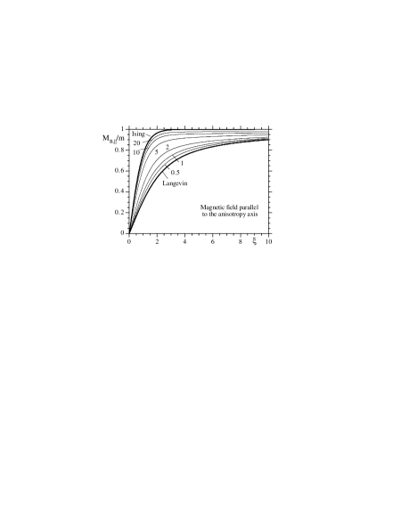
FIGURE 9.: Magnetization vs. longitudinal field $\xi=mB/k_{{\rm B}}T$ [Eq. (3.29)] for various values of the dimensionless anisotropy parameter $\sigma=Kv/k_{{\rm B}}T$, showing the anisotropy-induced non-$B/T$ superposition of the magnetization curves.

Finally, we shall compare the above results with other expressions derived for the magnetization. For $\sigma>0$, Eq. (3.29) reduces to the expression obtained by West (1961). Indeed, if we use the alternative expression (2.27) for ${\cal Z}_{\|}$ in terms of the Dawson integral $D$, we get

$$\frac{M_{B,\|}}{m}=\frac{1}{\sqrt{\sigma}}\,\frac{\sinh\xi}{e^{\xi}D(\sqrt{\sigma_{+}})+e^{-\xi}D(\sqrt{\sigma_{-}})}-\frac{\xi}{2\sigma}\;,$$ (3.30)

which is the result of West almost in its original form. Another formula was derived by Coffey, Cregg and Kalmykov (1993) when calculating relaxation times for magnetic nanoparticles by the effective eigenvalue method, namely

$$\frac{M_{B,\|}}{m}=\frac{\xi}{\sqrt{\sigma}\left[(\xi L(\xi)+1+\xi)D(\sqrt{\sigma}+\frac{\xi}{2\sqrt{\sigma}})+(\xi L(\xi)+1-\xi)D(\sqrt{\sigma}-\frac{\xi}{2\sqrt{\sigma}})\right]}-\frac{\xi}{2\sigma}\;,$$

where $L(\xi)$ is the Langevin function. However, on merely noting that $\sqrt{\sigma}\pm\xi/2\sqrt{\sigma}=\sqrt{\sigma_{\pm}}$, and using

$$\xi L(\xi)+1\pm\xi=\xi\coth\xi\pm\xi=\frac{\xi}{\sinh\xi}(\cosh\xi\pm\sinh\xi)=\frac{\xi}{\sinh\xi}e^{\pm\xi}\;,$$

their formula can be cast into the form (3.30) of West. Likewise the latter, the above alternative expression for $M_{B,\|}$ is written by assuming easy-axis anisotropy implicitly [recall the discussion as regards the validity of the expression (2.27) for ${\cal Z}_{\|}$].

2. General formula for the magnetization

On inserting the field expansion of the partition function (2.35) into the statistical-mechanical relation (3.24), the magnetization emerges in the form

$$M_{B}=m\sum_{i=1}^{\infty}\frac{2C_{i}}{(i-1)!}\xi^{2i-1}\bigg{/}\sum_{i=0}^{\infty}\frac{C_{i}}{i!}\xi^{2i}\;.$$ (3.31)

This formula gives a general expression for $M_{B}$ as a quotient of two series of powers of $\xi$ whose coefficients are expressible in terms of Kummer functions [Eq. (2.39)]. Such a mathematical object is clearly not easy to deal with. Nevertheless, one can check by an explicit identification of the corresponding series, that when the limit cases of the coefficients $C_{i}$ (see Table III) are introduced into Eq. (3.31), one gets the isotropic, Ising, and plane-rotator results for the magnetization. Indeed, for the series in the numerator and the denominator (the magnetic-field dependent factor in the partition function) we obtain

	$\sigma=0$	$\sigma\to\infty$	$\sigma\to-\infty$
$\sum_{i=1}^{\infty}\frac{2C_{i}}{(i-1)!}\xi^{2i-1}$	$\frac{1}{\xi}\left(\cosh\xi-\frac{1}{\xi}\sinh\xi\right)$	$\cos\alpha\sinh(\xi_{\|})$	$\sin\alpha I_{1}(\xi_{\perp})$
$\sum_{i=0}^{\infty}\frac{C_{i}}{i!}\xi^{2i}$	$\frac{1}{\xi}\sinh\xi$	$\cosh(\xi_{\|})$	$I_{0}(\xi_{\perp})$

Therefore, Eq. (3.31) contains, as particular cases, the limit formulae for the magnetization discussed above.

3. Series expansions of the magnetization

a. Expansion of the magnetization in powers of the anisotropy parameter.

Here we shall derive the magnetization from the weak-anisotropy expansion of the free energy obtained in Subsec. II.E. In this way, we shall arrive at an approximate analytical expression for $M_{B}$ that comprises the first corrections to the Langevin magnetization due to non-zero magnetic anisotropy.

To this end, we must differentiate the expansion of ${\cal F}$ in powers of $\sigma=Kv/k_{{\rm B}}T$ [Eq. (2.70)] with respect to the field. Prior to taking the $\xi$-derivatives of the first two coefficients of that expansion, we shall rewrite them in alternative forms. Equation (2.71) for ${\cal Z}_{1}/{\cal Z}_{0}$ can be written as

$$\frac{{\cal Z}_{1}}{{\cal Z}_{0}}=\cos^{2}\!\alpha-(3\cos^{2}\!\alpha-1)\frac{1}{\xi}L\;,$$

while Eq. (2.72) for the coefficient in $\sigma^{2}$ can be cast into the form

$$\frac{1}{2}\left[\frac{{\cal Z}_{2}}{{\cal Z}_{0}}-\left(\frac{{\cal Z}_{1}}{{\cal Z}_{0}}\right)^{2}\right] = (35\cos^{4}\!\alpha-30\cos^{2}\!\alpha+3)\frac{1}{2\xi^{2}}\left(1-\frac{3}{\xi}L\right)$$

$${}-(9\cos^{4}\!\alpha-6\cos^{2}\!\alpha+1)\frac{1}{2\xi^{2}}L^{2}-(\cos^{4}\!\alpha-\cos^{2}\!\alpha)\frac{2}{\xi}L\;.$$

Now, on taking the derivatives of the above coefficients with help form Eq. (2.54) for $(L/\xi)^{\prime}$, we get

$$\left(\frac{{\cal Z}_{1}}{{\cal Z}_{0}}\right)^{\prime} = (3\cos^{2}\!\alpha-1)\frac{1}{\xi}\left[L^{2}-\left(1-\frac{3}{\xi}L\right)\right]\;,$$ (3.32)

$$\frac{1}{2}\left[\frac{{\cal Z}_{2}}{{\cal Z}_{0}}-\left(\frac{{\cal Z}_{1}}{{\cal Z}_{0}}\right)^{2}\right]^{\prime} = (35\cos^{4}\!\alpha-30\cos^{2}\!\alpha+3)\frac{1}{2\xi^{3}}\left[3L^{2}-5\left(1-\frac{3}{\xi}L\right)\right]$$ (3.33)

$${}+(9\cos^{4}\!\alpha-6\cos^{2}\!\alpha+1)\frac{1}{\xi^{2}}L\left[L^{2}-\left(1-\frac{3}{\xi}L\right)\right]$$

$${}+(\cos^{4}\!\alpha-\cos^{2}\!\alpha)\frac{2}{\xi}\left[L^{2}-\left(1-\frac{3}{\xi}L\right)\right]\;.$$

These expressions, when introduced into

$$\frac{M_{B}}{m}\simeq L(\xi)+\left(\frac{{\cal Z}_{1}}{{\cal Z}_{0}}\right)^{\prime}\sigma+\frac{1}{2}\left[\frac{{\cal Z}_{2}}{{\cal Z}_{0}}-\left(\frac{{\cal Z}_{1}}{{\cal Z}_{0}}\right)^{2}\right]^{\prime}\sigma^{2}\;,$$ (3.34)

yield the first terms of the desired weak-anisotropy expansion of the magnetization.

Some relevant particular cases are those where the field points along the anisotropy axis, perpendicular to it, and when the anisotropy axes are distributed at random. In the first two cases we find

$$\frac{M_{B,\|}}{m} \simeq L(\xi)+\frac{2}{\xi}\left[L^{2}-\left(1-\frac{3}{\xi}L\right)\right]\sigma$$ (3.35)

$${}+\frac{4}{\xi^{3}}\left\{\left[3L^{2}-5\left(1-\frac{3}{\xi}L\right)\right]+\xi L\left[L^{2}-\left(1-\frac{3}{\xi}L\right)\right]\right\}\sigma^{2}\;,\qquad\quad$$

$$\frac{M_{B,\perp}}{m} \simeq L(\xi)-\frac{1}{\xi}\left[L^{2}-\left(1-\frac{3}{\xi}L\right)\right]\sigma$$ (3.36)

$${}+\frac{1}{\xi^{3}}\left\{\frac{3}{2}\left[3L^{2}-5\left(1-\frac{3}{\xi}L\right)\right]+\xi L\left[L^{2}-\left(1-\frac{3}{\xi}L\right)\right]\right\}\sigma^{2}\;,\qquad\quad$$

while $\langle M_{B}\rangle_{{\rm ran}}$ is obtained by introducing the averages (2.64) into Eqs. (3.32) and (3.33), getting

$$\frac{\left\langle M_{B}\right\rangle_{{\rm ran}}}{m}\simeq L(\xi)-\frac{4}{15}\left(1-\frac{3}{\xi}L\right)\frac{1}{\xi}\left[L^{2}-\left(1-\frac{3}{\xi}L\right)\right]\sigma^{2}\;.$$ (3.37)

Naturally, one can also obtain this result by taking the $\xi$-derivative of the $\sigma$-expansion of $\langle{\cal F}\rangle_{{\rm ran}}$ [Eq. (2.73)]. As was anticipated there, for anisotropy axes distributed at random, the corrections to the Langevin magnetization due to the magnetic anisotropy begin at second order.

In order to estimate the range of validity of the weak-anisotropy expansion of the magnetization, this has been compared with the exact analytical formula (3.29) for the longitudinal magnetization. It is shown in Fig. 10 that the approximate (3.35) works reasonably well up to $\sigma\sim 2$. Considering that the expansion has been performed by assuming $\sigma$ as the small parameter, the range of validity obtained is quite wide.

FIGURE 10.: Magnetization vs. longitudinal field $\xi=mB/k_{{\rm B}}T$ [Eq. (3.29); solid lines], along with the weak-anisotropy formula (3.35) (left panel, dashes) and the asymptotic formula (b.) (right panel, dashes), for various values of the dimensionless anisotropy parameter $\sigma=Kv/k_{{\rm B}}T$.

The effect of the orientation of the field with respect to the anisotropy axis is shown in Fig. 11. In contrast to the longitudinal-field case, where the anisotropy energy favors the alignment of the magnetic moment in the field direction, in the transverse case the anisotropy hinders the magnetization process, and the magnetization curve goes below the Langevin curve. In addition, for an ensemble of spins with anisotropy axes distributed at random, this phenomenon slightly dominates the favored alignment of the longitudinal-field case, so that the corresponding magnetization is slightly lower the Langevin magnetization.

FIGURE 11.: Upper panel: Magnetization vs. longitudinal field [Eq. (3.35)] and transverse field [Eq. (3.36)], and for anisotropy axes distributed at random [Eq. (3.37)]. Lower panel: Anisotropy induced contribution to the magnetization.

The anisotropy-induced contribution to the magnetization, $M_{B}(\xi)-mL(\xi)$, has been isolated in the lower panel of Fig. 11. This representation neatly shows that the random orientation of the anisotropy axes significantly reduces the anisotropy-induced contribution to the magnetization process. In the range of low fields, moreover, that significant reduction becomes an exact cancellation. This is due to the fact that the linear susceptibility is independent on the anisotropy energy when the anisotropy axes are distributed at random. This result, which was advanced when considering such an average of the field expansion of the free energy [Eq. (2.69)], is not restricted to the weak-anisotropy range (see Subsec. III.D).

We finally remark that for easy-plane anisotropy ($\sigma<0$), the results described are only slightly modified. Here, the longitudinal- and transverse-field cases, interchange in some sense their rôles. For $\vec{B}\parallel\hat{n}$ and $\sigma<0$, the magnetic anisotropy hinders the magnetization process, whereas this is naturally favored in the transverse field case. However, for anisotropy axes distributed at random, the net magnetization curve again goes slightly below the Langevin curve.

b. Asymptotic expansion of the magnetization for strong anisotropy.

We shall now derive the magnetization from the asymptotic expansion of the free energy for large $\sigma=Kv/k_{{\rm B}}T$. In this way, we shall obtain an analytical formula that contains the first corrections to the Ising-type magnetization due to non-infinite magnetic anisotropy.

We proceed by differentiating the $1/\sigma$-expansion of $\ln{\cal Z}$ [Eq. (2.74)] with respect to the field. The $\xi$-derivative of the coefficient of $1/\sigma$, reads

$$\left[(2+\xi_{\perp}^{2})-2\xi_{\|}\tanh\xi_{\|}\right]^{\prime}=-2\bigg{[}-\sin\alpha\xi_{\perp}+\cos\alpha\tanh\xi_{\|}+\frac{\cos\alpha\xi_{\|}}{\cosh^{2}\xi_{\|}}\bigg{]}\;,$$

where ${\rm d}\xi_{\|}/{\rm d}\xi=\cos\alpha$ and ${\rm d}\xi_{\perp}/{\rm d}\xi=\sin\alpha$ have been used. The $\xi$-derivative of the coefficient of $1/\sigma^{2}$ is taken similarly, yielding

$$\left[5+(2\xi_{\|}^{2}+\xi_{\perp}^{2})-(4+\xi_{\perp}^{2})\xi_{\|}\tanh\xi_{\|}-\xi_{\|}^{2}\tanh^{2}\xi_{\|}\right]^{\prime}$$

$$= -\cos\alpha\tanh\xi_{\|}\bigg{\{}4+3\xi_{\perp}^{2}-2\xi_{\|}\bigg{[}\tanh\xi_{\|}-\frac{\xi_{\|}}{\cosh^{2}\xi_{\|}}\bigg{]}\bigg{\}}$$

$${}+2\sin\alpha\xi_{\perp}-\cos\alpha\xi_{\perp}^{2}\frac{\xi_{\|}}{\cosh^{2}\xi_{\|}}\;.$$

On collecting these results and using $M_{B}=m(\partial\ln{\cal Z}/\partial\xi)$, the approximate magnetization can finally be written as

$$\frac{M_{B}}{m} \simeq \cos\alpha\tanh\xi_{\|}\Bigg{\{}1-\frac{1}{2\sigma}\left[1+\frac{2\xi_{\|}}{\sinh(2\xi_{\|})}\right]-\frac{1}{8\sigma^{2}}\left[4-\xi_{\|}\frac{\sinh(2\xi_{\|})-2\xi_{\|}}{\cosh^{2}\xi_{\|}}\right]\Bigg{\}}$$ (3.38)

$${}+\sin\alpha\xi_{\perp}\left(\frac{1}{2\sigma}+\frac{1}{4\sigma^{2}}\right)-\cos\alpha\xi_{\perp}^{2}\frac{3\sinh(2\xi_{\|})+2\xi_{\|}}{\cosh^{2}\xi_{\|}}\frac{1}{16\sigma^{2}}\;.$$

This formula extends the asymptotic result of Garanin (1996, Eq. (3.13)) in the longitudinal-field case ($\xi_{\|}=\xi$, $\xi_{\perp}=0$) to an arbitrary orientation of the field.

Let us explicitly write down the above approximate expression when the field points along the anisotropy axis and perpendicular to it, namely

$$\frac{M_{B,\|}}{m} \simeq \tanh\xi\left\{1-\frac{1}{2\sigma}\left[1+\frac{2\xi}{\sinh(2\xi)}\right]-\frac{1}{8\sigma^{2}}\left[4-\xi\frac{\sinh(2\xi)-2\xi}{\cosh^{2}\xi}\right]\right\}\;,$$

$$\frac{M_{B,\perp}}{m} \simeq \xi\left(\frac{1}{2\sigma}+\frac{1}{4\sigma^{2}}\right)\;.$$ (3.40)

Note that in the transverse-field case the leading (Ising) result is identically zero and one gets a linear increase of the magnetization with $\xi$. On the other hand, the occurrence of $\alpha$ in the arguments of the hyperbolic functions in Eq. (3.38), precludes the obtainment of a simple formula for $M_{B}$ when the anisotropy axes are distributed at random.

As we did when studying the magnetization for weak anisotropy, we may estimate the range of validity of the asymptotic expansion of $M_{B}$, by comparing it with the exact analytical formula for $M_{B,\|}$. Figure 10 also displays such a comparison showing that, for the field range considered, the approximation derived works reasonably well down to quite small values of $\sigma$. There is however an important difference with the weak-anisotropy formula for $M_{B}$, the accuracy of which was not significantly sensitive to the magnitude of the field. Here, all the approximate curves depart from the exact results at a certain value of the field, which decreases as the anisotropy does. The breaking down of the asymptotic expansion at high fields is apparent in the transverse-field case (3.40), which yields a linear dependence of $M_{B}$ on $\xi$, whereas at high fields the magnetization must saturate.

These limitations occur because of the $\sigma\gg 1$ expansions have as leading terms Ising-type results (i.e., they correspond to a potential with two deep minima), and the next-order terms are corrections associated with the finite curvature of the potential at the bottom of the wells. However, at sufficiently high fields the two-minima structure of the potential disappears (for example, for $B=B_{K}$ in a longitudinal field), and the expansion breaks down. In fact, already for $B\sim B_{K}/2$, which corresponds to $\xi\sim\sigma$ [see Eq. (2.6)], the upper potential well is quite shallow (see Fig. 1) and the inverse of the potential curvature at the minimum is large, so the expansion must already fail. This is consistent with the asymptotic results shown in Fig. 10: the approximate $M_{B}$ departs from the exact one at $\xi\sim 3$ for $\sigma=3$, at $\xi\sim 4$ for $\sigma=5$, at $\xi\sim 8$ for $\sigma=10$, and so on.

We finally mention that, as Fig. 10 suggests, the use of the weak-anisotropy formula, swapped at some point between $\sigma=2$ and $\sigma=5$ by the asymptotic expression, yields a reasonable approximation of the exact magnetization, except for the discrepancies discussed of the asymptotic $\xi\,\raisebox{1.50696pt}{$>$}\raisebox{-2.79857pt}{$\sim$}\,\sigma$ results. In this connection, as the $\sigma=3$ curve suggests, one can replace the asymptotic expansion for $\xi\,\raisebox{1.50696pt}{$>$}\raisebox{-2.79857pt}{$\sim$}\,\sigma$ by the weak-anisotropy formula in order to improve the overall approximation.

c. Field expansion of the magnetization.

Let us finally discuss the low-field expansion of the magnetization ($H=B/\mu_{0}$),

$$M_{B}=\chi_{1}H+\chi_{3}H^{3}+\chi_{5}H^{5}+\cdots\;,$$ (3.41)

which defines the linear, $\chi_{1}$ (or simply $\chi$), and non-linear, $\chi_{2n+1}$, $n=1,2,3,\ldots$, susceptibilities.

In order to derive general expressions for the susceptibilities, we can take the $\xi$-derivative of the low-$\xi$ expansion of $\ln{\cal Z}$ [Eq. (2.65)], getting

$$M_{B}=m \Big{[} 2C_{1}\xi+2(C_{2}-C_{1}^{2})\xi^{3}+(C_{3}-3C_{2}C_{1}+2C_{1}^{3})\xi^{5}$$ (3.42)

$${}+{\textstyle\frac{1}{3}}(C_{4}-4C_{3}C_{1}-3C_{2}^{2}+12C_{2}C_{1}^{2}-6C_{1}^{4})\xi^{7}+\cdots\Big{]}\;,$$

where the coefficients $C_{i}$ are given by Eqs. (2.36) or (2.39). One also arrives at Eq. (3.42) by expanding in powers of $\xi$ the inverse of the denominator of the general formula (3.31), and multiplying this expansion by the first terms of the series in the numerator.

TABLE V.: Combinations of the coefficients $C_{i}$ occurring in the first terms of the expansion (3.42) of the magnetization in powers of the magnetic field, in the isotropic, Ising, plane-rotator, and longitudinal-field cases.

	$\sigma=0$	$\sigma\to\infty$	$\sigma\to-\infty$	$\vec{B}\parallel\hat{n}$
${\scriptstyle 2C_{1}}$	$\frac{1}{3}$	$\cos^{2}\!\alpha$	${\textstyle\frac{1}{2}}\sin^{2}\!\alpha$	$\frac{R^{\prime}}{R}$
${\scriptstyle 2(C_{2}-C_{1}^{2})}$	$-\frac{1}{45}$	$-\frac{1}{3}\cos^{4}\!\alpha$	$-\frac{1}{16}\sin^{4}\!\alpha$	$\frac{1}{2}\left[\frac{1}{3}\frac{R^{\prime\prime}}{R}-\big{(}\frac{R^{\prime}}{R}\big{)}^{2}\right]$
${\scriptstyle C_{3}-3C_{2}C_{1}+2C_{1}^{3}}$	$\frac{2}{945}$	$\frac{2}{15}\cos^{6}\!\alpha$	$\frac{1}{96}\sin^{6}\!\alpha$	$\frac{1}{4}\left[\frac{1}{30}\frac{R^{\prime\prime\prime}}{R}-\frac{1}{2}\frac{R^{\prime\prime}}{R}\frac{R^{\prime}}{R}+\big{(}\frac{R^{\prime}}{R}\big{)}^{3}\right]$

The expansion (3.42) embodies $\chi$, $\chi_{3}$, $\chi_{5}$, and $\chi_{7}$; in general, $\chi_{2n+1}$ can be obtained by inserting the appropriate $C_{i}$ into the expression for the $n$th-order cumulant. The coefficients of the first three terms at $\sigma\to 0,\pm\infty$, and for $\vec{B}\parallel\hat{n}$, are given in Table V (they can be obtained from the expressions of Table IV). On inserting those coefficients into the above expansion of $M_{B}$, one gets the approximate formulae

$$M_{B,{\rm Lan}} = m\left[\frac{1}{3}\xi-\frac{1}{45}\xi^{3}+\frac{2}{945}\xi^{5}+\cdots\right]\;,$$ (3.43)

$$M_{B,{\rm Ising}} = m\cos\alpha\left[\xi_{\|}-\frac{1}{3}\xi_{\|}^{3}+\frac{2}{15}\xi_{\|}^{5}+\cdots\right]\;,$$ (3.44)

$$M_{B,{\rm rot}} = m\sin\alpha\left[{\textstyle\frac{1}{2}}\xi_{\perp}-\frac{1}{16}\xi_{\perp}^{3}+\frac{1}{96}\xi_{\perp}^{5}+\cdots\right]\;,$$ (3.45)

$$M_{B,\|} = m\Bigg{\{}\frac{R^{\prime}}{R}\xi+\frac{1}{2}\left[\frac{1}{3}\frac{R^{\prime\prime}}{R}-\bigg{(}\frac{R^{\prime}}{R}\bigg{)}^{2}\right]\xi^{3}$$ (3.46)

$$\hskip 17.50002pt{}+\frac{1}{4}\left[\frac{1}{30}\frac{R^{\prime\prime\prime}}{R}-\frac{1}{2}\frac{R^{\prime\prime}}{R}\frac{R^{\prime}}{R}+\bigg{(}\frac{R^{\prime}}{R}\bigg{)}^{3}\right]\xi^{5}+\cdots\Bigg{\}}\;.\qquad$$

Note that, in the first three cases $\chi_{2n+1}$ depends on $T$ with a $T^{-(2n+1)}$ law. This is the translation to linear and non-linear susceptibilities of the $B/T$ superposition of the corresponding magnetization curves. Outside these limit ranges, however, the temperature dependence of $C_{i}(\sigma,\alpha)$ through $\sigma$, provokes that $\chi_{2n+1}(T)$ no longer satisfies such a simple $T^{-(2n+1)}$ law. This is already illustrated by the above expansion of $M_{B,\|}$, in which it can be recognized the extra dependence of the susceptibilities on $T$, provided by the functions $R^{(\ell)}(\sigma)/R(\sigma)$ via $\sigma$.

These points will be further investigated in the following two subsections devoted to the linear and non-linear susceptibilities, respectively.

III.D Linear susceptibility

We shall now study the linear susceptibility of classical spins with axially symmetric magnetic anisotropy. The linear susceptibility, $\chi$, can be defined as the coefficient of the linear term in the expansion of the magnetization in powers of the external field. On comparing the $H$-expansion of $M_{B}$ (3.41) with the $\xi$-expansion (3.42), and using $\xi=\mu_{0}mH/k_{{\rm B}}T$, one gets the following expression for $\chi$

$$\chi=\frac{\mu_{0}m^{2}}{k_{{\rm B}}T}2C_{1}(\sigma,\alpha)\;,$$ (3.47)

which involves the first coefficient in the expansion of the partition function in powers of $\xi$. Recall that $\alpha$ is the angle between the anisotropy axis $\hat{n}$ and the field, while $\sigma=Kv/k_{{\rm B}}T$.

1. Linear susceptibility: particular cases

Let us first consider the expressions that emerge from Eq. (3.47) when one inserts the particular cases of $2C_{1}$ into it (Table V).

a. Isotropic case.

For $\sigma\to 0$, $2C_{1}=1/3$, whence one gets the Curie law for the susceptibility

$$\chi_{{\rm Lan}}=\frac{\mu_{0}m^{2}}{3k_{{\rm B}}T}\;.$$ (3.48)

For classical spins, this result naturally follows from the absence of anisotropy.

b. Ising regime.

For $\sigma\to\infty$, $2C_{1}=\cos^{2}\!\alpha$, so that

$$\chi_{{\rm Ising}}=\frac{\mu_{0}m^{2}}{k_{{\rm B}}T}\cos^{2}\!\alpha\;,$$ (3.49)

which is analogous to the susceptibility of an Ising spin. Thus, when the field points along a direction perpendicular to the “Ising axis” ($\cos\alpha=0$), $\chi$ vanishes.

c. Plane-rotator regime.

For $\sigma\to-\infty$, $2C_{1}=\sin^{2}\!\alpha/2$, so that the plane-rotator linear susceptibility is given by

$$\chi_{{\rm rot}}=\frac{\mu_{0}m^{2}}{2k_{{\rm B}}T}\sin^{2}\!\alpha\;.$$ (3.50)

In this case the response is identically zero when the field points perpendicular to the easy plane.

d. Longitudinal-field case.

On introducing $2C_{1}|_{\alpha=0}=R^{\prime}/R$ in Eq. (3.47) one gets the longitudinal susceptibility

$$\chi_{\|}=\frac{\mu_{0}m^{2}}{k_{{\rm B}}T}\frac{R^{\prime}}{R}\;,$$ (3.51)

where the factor $R^{\prime}/R$ induces an extra dependence on $T$ via $\sigma$, “interpolating” between the isotropic ($R^{\prime}/R|_{\sigma=0}=1/3$) and Ising ($R^{\prime}/R|_{\sigma\to\infty}=1$) results.

2. Formulae for the linear susceptibility

When the general expression (2.66) for $C_{1}$ is introduced into Eq. (3.47), the linear susceptibility emerges in the form

$$\chi=\frac{\mu_{0}m^{2}}{k_{{\rm B}}T}\left(\frac{R^{\prime}}{R}\cos^{2}\!\alpha+\frac{R-R^{\prime}}{2R}\sin^{2}\!\alpha\right)\;.$$ (3.52)

It is convenient to introduce the longitudinal and transverse components of $\chi$ (which are related with the diagonal elements of the susceptibility tensor; see below)

$$\chi_{\|}=\frac{\mu_{0}m^{2}}{k_{{\rm B}}T}\frac{R^{\prime}}{R}\;,\qquad\chi_{\perp}=\frac{\mu_{0}m^{2}}{k_{{\rm B}}T}\frac{R-R^{\prime}}{2R}\;,$$ (3.53)

so that $\chi$ can be written as

$$\chi=\chi_{\|}\cos^{2}\!\alpha+\chi_{\perp}\sin^{2}\!\alpha\;.$$ (3.54)

The quantities $\chi_{\|}$ and $\chi_{\perp}$ characterize, respectively, the equilibrium response to a longitudinal (parallel to $\hat{n}$) and transverse (perpendicular to $\hat{n}$) probing field. Due to the linearity of the response, when the probing field points along an arbitrary direction, the projection of the response along the probing-field direction in given by the weighted sum (3.54) of the longitudinal and transverse responses.

Other derivations of the equilibrium linear susceptibility of a dipole moment in the simplest axially symmetric anisotropy potential were carried out by Lin (1961), Raĭkher and Shliomis (1975) (see also Shliomis and Stepanov, 1993), Shcherbakova (1978), and Chantrell et al. (1985).

a. Average of the linear susceptibility for anisotropy axes distributed at random.

For an ensemble of equivalent magnetic moments (i.e., with the same characteristic parameters) whose anisotropy axes are distributed at random, one finds

$$\left\langle\chi\right\rangle_{{\rm ran}}=\frac{\mu_{0}m^{2}}{k_{{\rm B}}T}\left(\frac{R^{\prime}}{R}\frac{1}{3}+\frac{R-R^{\prime}}{2R}\frac{2}{3}\right)=\frac{\mu_{0}m^{2}}{3k_{{\rm B}}T}\;,$$ (3.55)

which is merely the Curie law for the linear susceptibility. This equation entails that, irrespective of the magnitude of the magnetic anisotropy as compared with the thermal energy, the linear susceptibility of the randomly oriented ensemble is equal to the susceptibility of isotropic magnetic moments. This also holds in the extreme anisotropy cases: for an ensemble of Ising spins, with Ising axes distributed at random, $\langle\chi_{{\rm Ising}}\rangle_{{\rm ran}}=\mu_{0}m^{2}/3k_{{\rm B}}T$; likewise, for an ensemble of plane rotators, with axes of rotation distributed at random, $\langle\chi_{{\rm rot}}\rangle_{{\rm ran}}$ is given by the Curie law (3.55).

We shall see below that Eq. (3.55) is in fact rather general; it holds whenever the Hamiltonian of the spin (in the absence of the probing field) has inversion symmetry ($\vec{m}\leftrightarrow-\vec{m}$).

b. Reduced linear susceptibility.

An informative quantity is the reduced linear susceptibility defined as $\chi^{{\rm red}}=\chi(k_{{\rm B}}T/\mu_{0}m^{2})=2C_{1}$, whence

$$\chi^{{\rm red}}(\sigma,\alpha)=\frac{R^{\prime}}{R}\cos^{2}\!\alpha+\frac{R-R^{\prime}}{2R}\sin^{2}\!\alpha\;.$$ (3.56)

This quantity has the property that isolates the temperature-dependence of $\chi$ induced by the magnetic anisotropy. Besides, it embodies the angular dependence of $\chi$. Figure 12 shows $\chi^{{\rm red}}$ as a function of the angle between the anisotropy axis and the probing field (cf. Lin, 1961). As expected, the larger the $|\sigma|$, the more anisotropic the $\chi^{{\rm red}}$ curves, becoming rather different from circles already for $|\sigma|\simeq 5$.

FIGURE 12.: Polar plots showing the angular dependence of the reduced linear susceptibility $\chi^{{\rm red}}$ [Eq. (3.56)] for various values of the dimensionless anisotropy parameter $\sigma=Kv/k_{{\rm B}}T$. (a) Easy-axis anisotropy. (b) Easy-plane anisotropy.

Figure 13 shows $\chi^{{\rm red}}$ for the longitudinal and transverse components of the linear susceptibility (in this representation $\langle\chi^{{\rm red}}\rangle_{{\rm ran}}$ would take the constant value $1/3$). Both curves coincide for $\sigma=0$, where the orientation of the field plays no rôle, taking the Langevin value $1/3$. It can also be seen that the maximum variation of $\chi^{{\rm red}}$ with $\sigma$, occurs when the probing field is parallel to the anisotropy axis. Note also that, qualitatively, the longitudinal- and the transverse-field cases interchange their rôles when the sign of the anisotropy is reversed. This statement, which is supported by Fig. 12, is associated with the qualitatively “equivalent” magnetization behavior in the easy-axis and easy-plane anisotropy cases when the probing field points in the “easy-magnetization region” or in the “hard-magnetization region,” regions that interchange themselves when the sign of the anisotropy is changed.

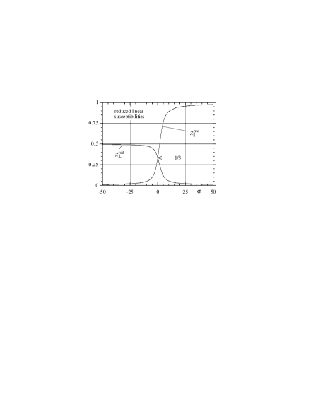
FIGURE 13.: Reduced linear susceptibility (3.56) in the longitudinal, $\chi_{\|}^{{\rm red}}$, and transverse, $\chi_{\perp}^{{\rm red}}$, field cases vs. the dimensionless anisotropy parameter $\sigma=Kv/k_{{\rm B}}T$ (cf. Fig. 6).

3. Generalizations

a. Probing-field derivative of the magnetization.

The definition of the linear susceptibility as the coefficient of the linear term in the expansion of the magnetization in powers of the external field, of course agrees with that in terms of the field derivative of the magnetization at zero field, i.e., $\chi=\mu_{0}[\partial\big{\langle}\vec{m}\cdot\hat{b}\big{\rangle}_{{\rm e}}/\partial B]\big{|}_{B=0}$. This definition suggests the immediate generalization

$$\chi=\mu_{0}\left.\frac{\partial\big{\langle}\vec{m}\cdot\hat{b}\big{\rangle}}{\partial(\Delta B)}\right|_{\Delta B=0}\;,$$ (3.57)

where $\Delta\vec{B}=\Delta B\,\hat{b}$ is an external probing field ($\hat{b}$ stands now for the unit vector in the direction of the probing field). The absence of the subscript “${\rm e}$” in the thermal-equilibrium averages is used to indicate that they are taken with respect to the total energy (system plus perturbation). The unperturbed system can already be subjected to a constant (bias) field, $\vec{B}$, not necessarily collinear with $\Delta\vec{B}$.

Indeed, the calculation of the linear susceptibility can be carried out by starting from a total Hamiltonian ${\cal H}_{\rm T}={\cal H}-\vec{m}\cdot\Delta\vec{B}$, where the knowledge of the actual form of ${\cal H}$ is not required. Let us calculate first

$$\frac{\partial\big{\langle}(\vec{m}\cdot\hat{b})^{n}\big{\rangle}}{\partial(\Delta B)}=\frac{\partial\;\;}{\partial(\Delta B)}\frac{\int\!{\rm d}{\Omega}\,(\vec{m}\cdot\hat{b})^{n}e^{-\beta{\cal H}_{\rm T}}}{\int\!{\rm d}{\Omega}\,e^{-\beta{\cal H}_{\rm T}}}$$

$$= \beta\,\frac{{\cal Z}\int\!{\rm d}{\Omega}\,(\vec{m}\cdot\hat{b})^{n+1}e^{-\beta{\cal H}_{\rm T}}-\int\!{\rm d}{\Omega}\,(\vec{m}\cdot\hat{b})^{n}e^{-\beta{\cal H}_{\rm T}}\int\!{\rm d}{\Omega}\,(\vec{m}\cdot\hat{b})e^{-\beta{\cal H}_{\rm T}}}{{\cal Z}^{2}}\;,$$

where as usual $\int\!{\rm d}{\Omega}\,(\cdot)=(1/2\pi)\int_{-1}^{1}\!{\rm d}{(\cos\vartheta)}\,\int_{0}^{2\pi}\!{\rm d}{\varphi}\,(\cdot)$. From the above result we get the general relation

$$\frac{\partial\big{\langle}(\vec{m}\cdot\hat{b})^{n}\big{\rangle}}{\partial(\Delta B)}=\beta\left[\big{\langle}(\vec{m}\cdot\hat{b})^{n+1}\big{\rangle}-\big{\langle}(\vec{m}\cdot\hat{b})^{n}\big{\rangle}\big{\langle}\vec{m}\cdot\hat{b}\big{\rangle}\right]\;,$$ (3.58)

the $n=1$ particular case of which merely reads

$$\frac{\partial\big{\langle}\vec{m}\cdot\hat{b}\big{\rangle}}{\partial(\Delta B)}=\beta\left[\big{\langle}(\vec{m}\cdot\hat{b})^{2}\big{\rangle}-\big{\langle}\vec{m}\cdot\hat{b}\big{\rangle}^{2}\right]\;,$$ (3.59)

and holds irrespective of the magnitude of $\Delta\vec{B}$. When this equation is evaluated at $\Delta B=0$ and inserted in Eq. (3.57), one gets the celebrated expression for the linear susceptibility in terms of the statistics of the thermal-equilibrium fluctuations of the magnetic moment in the absence of the probing field, namely

$$\chi=\frac{\mu_{0}}{k_{{\rm B}}T}\left[\big{\langle}(\vec{m}\cdot\hat{b})^{2}\big{\rangle}_{{\rm e}}-\big{\langle}\vec{m}\cdot\hat{b}\big{\rangle}_{{\rm e}}^{2}\right]\;,$$ (3.60)

where $\langle\,\rangle_{{\rm e}}$ denotes the equilibrium average in the absence of the perturbation.

The relation (3.60) is valid for any form of the Hamiltonian. When ${\cal H}$ is given by ${\cal H}=-(Kv/m^{2})(\vec{m}\cdot\hat{n})^{2}$ [cf. Eq. (2.2)], the above averages in the absence of the probing field are in fact zero-field averages, which are directly related with the coefficients $C_{i}$ by Eq. (2.42). Thus, by inserting

$$\big{\langle}\vec{m}\cdot\hat{b}\big{\rangle}_{{\rm e}}\big{|}_{B=0}=0\;,\qquad\big{\langle}(\vec{m}\cdot\hat{b})^{2}\big{\rangle}_{{\rm e}}\big{|}_{B=0}=m^{2}2C_{1}\;,$$

into Eq. (3.60), one recovers the expression (3.47) for $\chi$.

b. Tensor structure.

The linear susceptibility is in fact a tensor defined by

$$\chi_{ij}=\mu_{0}\left.\frac{\partial\left\langle m_{i}\right\rangle}{\partial(\Delta B_{j})}\right|_{\Delta B=0}\;.$$ (3.61)

Note that the diagonal elements are given by Eq. (3.57) when $\hat{b}$ points along $\hat{x}$, $\hat{y}$, and $\hat{z}$. By a derivation analogous to that leading to Eq. (3.60), one arrives at the result

$$\chi_{ij}=\frac{\mu_{0}}{k_{{\rm B}}T}\left[\left\langle m_{i}m_{j}\right\rangle_{{\rm e}}-\left\langle m_{i}\right\rangle_{{\rm e}}\left\langle m_{j}\right\rangle_{{\rm e}}\right]\;.$$ (3.62)

Owing to the fact that $\chi_{ij}$ is a symmetrical second-rank tensor, it can be diagonalized by a suitable change of coordinates. Let us assume that this diagonalization has already been carried out. Then, if a probing field $\Delta\vec{B}=\Delta B\,\hat{b}$ is applied, the projection of the average magnetic moment onto $\hat{b}$ is given in the linear response range by (we use $\mu_{0}\langle m_{i}\rangle\simeq\mu_{0}\langle m_{i}\rangle|_{\Delta B=0}+\sum_{j}\chi_{ij}\Delta B_{j}+\cdots$)

$$\mu_{0}\Delta\big{\langle}\vec{m}\big{\rangle}\cdot\hat{b}\simeq\left(\chi_{xx}\cos^{2}\!\alpha+\chi_{yy}\cos^{2}\!\beta+\chi_{zz}\cos^{2}\!\gamma\right)\Delta B\;,$$ (3.63)

where $(\alpha,\beta,\gamma)$ are the direction cosines of $\hat{b}$ (in the coordinate system that diagonalizes $\chi_{ij}$). The quantity into the brackets defines an effective linear susceptibility $\chi$, which is in fact what we have been calling linear susceptibility throughout.

c. The average of the linear susceptibility for anisotropy axes distributed at random revisited.

On the basis of the above expressions, we can derive the result mentioned for the linear susceptibility of an ensemble of equivalent dipole moments whose Hamiltonian has inversion symmetry and their intrinsic axes are distributed at random.

For an ensemble of independent dipole moments, the contribution of each dipole to $\chi$ is analogous to that occurring in Eq. (3.63), with (in principle) different direction cosines and diagonal elements $\chi_{ii}$ for each dipole. However, if these elements are equal we can write the total effective susceptibility as

$$\chi=\chi_{xx}\left\langle\cos^{2}\!\alpha\right\rangle+\chi_{yy}\left\langle\cos^{2}\!\beta\right\rangle+\chi_{zz}\left\langle\cos^{2}\!\gamma\right\rangle\;,$$ (3.64)

where $\langle\,\rangle$ denotes average over the ensemble of dipoles. Note that for the assumption about the equality of the tensor elements to hold, the dipole moments must be equivalent (in the sense of having the same characteristic parameters) and the orientation of the intrinsic axes (which diagonalize the linear susceptibility tensor for each $\vec{m}$) with respect to the main reference frame, must be irrelevant in determining the $\chi_{ii}$; this excludes, for instance, the occurrence of an external (bias) field. Then, if those intrinsic axes are distributed at random, the effective linear susceptibility (3.64) reads

$$\left\langle\chi\right\rangle_{{\rm ran}}=\frac{1}{3}\left(\chi_{xx}+\chi_{yy}+\chi_{zz}\right)=\frac{\mu_{0}}{3k_{{\rm B}}T}\left\{m^{2}-\left[\left\langle m_{x}\right\rangle_{{\rm e}}^{2}+\left\langle m_{y}\right\rangle_{{\rm e}}^{2}+\left\langle m_{z}\right\rangle_{{\rm e}}^{2}\right]\right\}\;,$$

where Eq. (3.62) has been used to express the $\chi_{ii}$. Finally, if the Hamiltonian of each dipole has inversion symmetry ($\langle m_{i}^{2n+1}\rangle_{{\rm e}}=0$), one has $\langle m_{i}\rangle_{{\rm e}}=0$, $i=x,y,z$, so that the above formula reduces to

$$\left\langle\chi\right\rangle_{{\rm ran}}=\frac{\mu_{0}m^{2}}{3k_{{\rm B}}T}\;,$$ (3.65)

(note that presence of a bias field could as well be excluded on the basis of the inversion-symmetry condition). Equation (3.65) is the announced result: for an ensemble of equivalent dipole moments whose Hamiltonian has inversion symmetry, the effective linear susceptibility is given by the Curie law when their intrinsic axes are distributed at random.

d. General formula for any axially symmetric Hamiltonian.

We shall now calculate the linear susceptibility of a magnetic moment with an arbitrary axially symmetric Hamiltonian. The corresponding equilibrium probability distribution of $z=m_{z}/m$ is given by [cf. Eq. (2.26)]

$$P_{{\rm e},\|}(z)={\cal Z}_{\|}^{-1}\exp[-\beta{\cal H}(z)]\;,\qquad{\cal Z}_{\|}=\int_{-1}^{1}\!\!{\rm d}{z}\,\exp[-\beta{\cal H}(z)]\;,$$ (3.66)

where we have assumed that the symmetry axis points along $\hat{z}$. In such a reference frame, the susceptibility tensor is diagonal and the diagonal elements are given by

$$\chi_{ii}=\frac{\mu_{0}}{k_{{\rm B}}T}\left[\left\langle m_{i}^{2}\right\rangle_{{\rm e}}-\left\langle m_{i}\right\rangle_{{\rm e}}^{2}\right]\;,\quad i=x,y,\mbox{~{}and~{}}z\;.$$ (3.67)

Besides, due to the axial symmetry of the Hamiltonian, the susceptibility tensor has only two independent elements $\chi_{\|}=\chi_{zz}$ and $\chi_{\perp}=\chi_{xx}=\chi_{yy}$.

Let us introduce the averages of the Legendre polynomials $p_{n}(z)$,

$$\begin{array}[]{rclrcl}p_{1}(z)&=&z\;,&p_{2}(z)&=&{\textstyle\frac{1}{2}}(3z^{2}-1)\;,\\ p_{3}(z)&=&{\textstyle\frac{1}{2}}(5z^{3}-3z)\;,&p_{4}(z)&=&\frac{1}{8}(35z^{4}-30z^{2}+3)\;,\ldots\end{array}$$ (3.68)

with respect to the equilibrium probability distribution $P_{{\rm e},\|}(z)$, namely

$$S_{n}\stackrel{{\scriptstyle{\rm def}}}{{=}}\left\langle p_{n}(z)\right\rangle_{{\rm e}}=\int_{-1}^{1}\!\!{\rm d}{z}\,p_{n}(z)P_{{\rm e},\|}(z)\;.$$ (3.69)

In terms of these quantities, we can write $\chi_{\|}$ and $\chi_{\perp}$ as

$$\chi_{\|}=\frac{\mu_{0}m^{2}}{k_{{\rm B}}T}\left(\frac{1+2S_{2}}{3}-S_{1}^{2}\right)\;,\qquad\chi_{\perp}=\frac{\mu_{0}m^{2}}{k_{{\rm B}}T}\frac{1-S_{2}}{3}\;,$$ (3.70)

for the writing of which we have employed

$$\begin{array}[]{rclrcl}\left\langle m_{z}\right\rangle_{{\rm e}}&=&mS_{1}\;,&\left\langle m_{z}^{2}\right\rangle_{{\rm e}}&=&m^{2}(1+2S_{2})/3\;,\\ \left\langle m_{x,y}\right\rangle_{{\rm e}}&=&0\;,&\left\langle m_{x,y}^{2}\right\rangle_{{\rm e}}&=&\left(m^{2}-\left\langle m_{z}^{2}\right\rangle_{{\rm e}}\right)/2\;.\end{array}$$

The above expressions for $\chi$ are valid, for example, for any axially symmetric anisotropy potential in a longitudinal bias field. For the simplest uniaxial anisotropy in a longitudinal bias field

$$-\beta{\cal H}=\sigma z^{2}+\xi z\;,$$ (3.71)

one can derive the following explicit expressions for $S_{1}$ and $S_{2}$

$$S_{1} = \frac{e^{\sigma}}{\sigma{\cal Z}_{\|}}\sinh\xi-h\;,$$ (3.72)

$$S_{2} = \frac{3}{2}\left[\frac{e^{\sigma}}{\sigma{\cal Z}_{\|}}(\cosh\xi-h\sinh\xi)+h^{2}-\frac{1}{2\sigma}\right]-\frac{1}{2}\;,$$ (3.73)

where $h=B/B_{K}=\xi/2\sigma$ and ${\cal Z}_{\|}$ is given by Eq. (2.25).

In the $K=0$ case, the linear susceptibility is more easily obtained directly from the definition (3.69) of the $S_{n}$ with help from Eqs. (2.46)–(2.51). On doing so, one obtains

$$\chi_{\|}=\frac{\mu_{0}m^{2}}{k_{{\rm B}}T}L^{\prime}\;,\qquad\chi_{\perp}=\frac{\mu_{0}m^{2}}{k_{{\rm B}}T}\frac{1}{\xi}L\;,$$ (3.74)

where $L(\xi)$ is the Langevin function. Note that, since $L(\xi)=\xi/3+\cdots$ for low fields [Eq. (3.43)], both components of the above formula merge on the Curie law $\chi=\mu_{0}m^{2}/3k_{{\rm B}}T$ as the bias field goes to zero.

For $B=0$, the linear susceptibility is sometimes found written in a number of alternative forms. Note first that in this case one has $S_{1}=0$. Therefore, on introducing the notation $\tilde{S}_{2}=S_{2}(\sigma,\xi)|_{\xi=0}$, one gets from Eq. (3.70) the following formulae

$$\chi_{\|}=\frac{\mu_{0}m^{2}}{k_{{\rm B}}T}\frac{1+2\tilde{S}_{2}}{3}\;,\qquad\chi_{\perp}=\frac{\mu_{0}m^{2}}{k_{{\rm B}}T}\frac{1-\tilde{S}_{2}}{3}\;.$$ (3.75)

(The quantity $\tilde{S}_{2}$ is sometimes written as $S$ or merely $S_{2}$.) In order to directly check Eqs. (3.75) against Eqs. (3.53) one only needs to use

$$\frac{R^{\prime}}{R}=\frac{\int_{-1}^{1}\!{\rm d}{z}\,z^{2}\exp(\sigma z^{2})}{\int_{-1}^{1}\!{\rm d}{z}\,\exp(\sigma z^{2})}=\left.\left\langle z^{2}\right\rangle_{{\rm e}}\right|_{B=0}=\frac{1}{3}\left.(1+2S_{2})\right|_{B=0}=\frac{1}{3}(1+2\tilde{S}_{2})\;.$$ (3.76)

Alternative expressions for $\chi$ at $B=0$ can also be written in terms of Kummer functions. Thus, on introducing $C_{1}$ from Eq. (2.41) into Eq. (3.47), one directly gets (cf. Coffey, Crothers, Kalmykov and Waldron, 1995b)

$$\chi_{\|}=\frac{\mu_{0}m^{2}}{3k_{{\rm B}}T}\frac{M({\textstyle\frac{3}{2}},{\textstyle\frac{5}{2}};\sigma)}{M({\textstyle\frac{1}{2}},{\textstyle\frac{3}{2}};\sigma)}\;,\qquad\chi_{\perp}=\frac{\mu_{0}m^{2}}{3k_{{\rm B}}T}\frac{M({\textstyle\frac{1}{2}},{\textstyle\frac{5}{2}};\sigma)}{M({\textstyle\frac{1}{2}},{\textstyle\frac{3}{2}};\sigma)}\;.$$ (3.77)

4. Approximate formulae for the linear susceptibility

We shall now derive approximate formulae for $\chi$ with the aim of by-pass, when possible, the use of expressions involving non-elementary functions. The formulae obtained, based on weak- and strong-anisotropy expansions, reasonably compare with the exact results in whole temperature range.

We find it convenient to rewrite first the exact expression (3.52) for $\chi$ as follows

$$\chi=\frac{\mu_{0}m^{2}}{k_{{\rm B}}T}\frac{1}{3}\left[1+\frac{1}{2}\left(3\frac{R^{\prime}}{R}-1\right)(3\cos^{2}\!\alpha-1)\right]\;,$$ (3.78)

where the factor multiplying $(3\cos^{2}\!\alpha-1)$ is precisely $\tilde{S}_{2}$ [see Eq. (3.76)]. In order to derive approximate formulae for $\chi$ in the unbiased case we shall use the approximate results for $R^{\prime}/R$ derived in Appendix A. We can also get most of the following results (up to second order) if we start from the expansions of $M_{B}$ in powers of $\sigma$ [Eq. (3.34)] and the asymptotic expansion (3.38).

a. Weak-anisotropy range.

In order to obtain an approximate formula for $\chi$ valid in the $|\sigma|\ll 1$ range, we insert the approximate $R^{\prime}/R$ from Eq. (a) into Eq. (3.78), getting

$$\left.\chi\right|_{|\sigma|\ll 1}\simeq\frac{\mu_{0}m^{2}}{3k_{{\rm B}}T}\left[1+\left(\frac{2}{15}\sigma+\frac{4}{315}\sigma^{2}-\frac{8}{4725}\sigma^{3}\right)(3\cos^{2}\!\alpha-1)\right]\;.$$ (3.79)

This equation yields a good approximation of the exact $\chi$ for $|\sigma|\leq 2$. Note that, as it should, when the anisotropy axes are distributed at random, the corrections to the leading (isotropic) result vanish at all orders.

b. Strong-anisotropy ranges.

Similarly, to obtain approximate formulae for $\chi$ valid in the $|\sigma|\gg 1$ ranges, we shall use the corresponding approximate expressions for $R^{\prime}/R$ derived in Appendix A.

For $\sigma\ll-1$, we insert $R^{\prime}/R$ from Eq. (A.28) into Eq. (3.78), getting

$$\left.\chi\right|_{\sigma\ll-1}\simeq\frac{\mu_{0}m^{2}}{k_{{\rm B}}T}\left[\frac{1}{2}\sin^{2}\!\alpha-\frac{1}{4\sigma}(3\cos^{2}\!\alpha-1)\right]\;.$$ (3.80)

An approximate formula for the extreme easy-axis case can be derived in a similar way. On substituting the $\sigma\gg 1$ result (b) for $R^{\prime}/R$ in Eq. (3.78), we obtain

$$\left.\chi\right|_{\sigma\gg 1}\simeq\frac{\mu_{0}m^{2}}{k_{{\rm B}}T}\left[\cos^{2}\!\alpha-\left(\frac{1}{2\sigma}+\frac{1}{4\sigma^{2}}+\frac{5}{8\sigma^{3}}\right)(3\cos^{2}\!\alpha-1)\right]\;.$$ (3.81)

Again, when the anisotropy axes are distributed at random, all the corrections to the leading plane-rotator and Ising results vanish identically. These approximate formulae compare well with the corresponding exact results for $|\sigma|\geq 5$, so that, on complementing Eqs. (3.79), (3.80), and (3.81) one can cover the entire $\sigma$-range reasonably. This merely follows from the patching (shown in Fig. 34 of Appendix A) of the exact $R^{\prime}/R$ provided by the approximate formulae with which the above approximate results for $\chi$ have been constructed.

For future reference, we finally write down the longitudinal and transverse components of $\chi$ for strong anisotropy to order $1/|\sigma|$, namely

$$\chi_{\|}\simeq\frac{\mu_{0}m^{2}}{k_{{\rm B}}T}-\frac{\mu_{0}m^{2}}{Kv}\;,\qquad\chi_{\perp}\simeq\frac{\mu_{0}m^{2}}{2Kv}\;,\qquad(K>0)\;,$$ (3.82)

and

$$\chi_{\|}\simeq\frac{\mu_{0}m^{2}}{2|K|v}\;,\qquad\chi_{\perp}\simeq\frac{\mu_{0}m^{2}}{2k_{{\rm B}}T}-\frac{\mu_{0}m^{2}}{4|K|v}\;,\qquad(K<0)\;.$$ (3.83)

Note the qualitative interchange of the rôles of $\chi_{\|}$ and $\chi_{\perp}$ with the transformation $K\to-K$.

c. Formulae in the presence of a longitudinal bias field.

We can also obtain high-barrier approximations of the exact equilibrium susceptibilities in the presence of a longitudinal bias field. Those equations, which will be valid for $h\ll 1$, can be obtained by starting from the approximate expression (2.28) for the partition function. Thus, on applying the relations [readily obtainable from Eqs. (3.66) and (3.69)]

$$S_{1}=\frac{1}{{\cal Z}_{\|}}\frac{\partial{\cal Z}_{\|}}{\partial\xi}\;,\qquad\frac{1}{3}(1+2S_{2})=\frac{1}{{\cal Z}_{\|}}\frac{\partial{\cal Z}_{\|}}{\partial\sigma}\;,$$ (3.84)

to the approximate ${\cal Z}_{\|}$ mentioned, one gets from Eqs. (3.70)

$$\chi_{\|} \simeq \frac{\mu_{0}m^{2}}{k_{{\rm B}}T}\frac{1}{(\cosh\xi-h\sinh\xi)^{2}}$$ (3.85)

$${}\times\bigg{\{}(1-h^{2})-\frac{1}{\sigma}+\frac{1}{8\sigma^{2}}\bigg{[}1-\frac{1+6h^{2}+h^{4}}{(1-h^{2})^{2}}\cosh(2\xi)$$

$$\hskip 120.00018pt{}+\frac{4h(1+h^{2})}{(1-h^{2})^{2}}\sinh(2\xi)\bigg{]}\bigg{\}}\;,$$

$$\chi_{\perp} \simeq \frac{\mu_{0}m^{2}}{k_{{\rm B}}T}\frac{1}{2\sigma}\frac{(1+h^{2})\cosh\xi-2h\sinh\xi}{(1-h^{2})(\cosh\xi-h\sinh\xi)}\;.$$ (3.86)

For $B=0$, these formulae duly reduce to Eqs. (3.82). Finally, on taking formally the $K\to\infty$ limit in these formulae (i.e., $\sigma\to\infty$ and $h=\xi/2\sigma\to 0$), one gets the “Ising-type” equilibrium susceptibilities in a longitudinal bias field [cf. Eq. (3.49)]

$$\chi_{\|}\simeq\frac{\mu_{0}m^{2}}{k_{{\rm B}}T}\frac{1}{\cosh^{2}\xi}\;,\qquad\chi_{\perp}\simeq 0\;.$$ (3.87)

Equations (3.85), (3.86), and (3.87) will be used in Section V.

5. Temperature dependence of the linear susceptibility

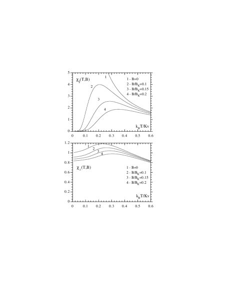
FIGURE 14.: Longitudinal and transverse components of the linear susceptibility vs. $T$ in the unbiased case and in the presence of longitudinal bias fields [Eqs. (3.70)]. The anisotropy is assumed to be of easy-axis type ($K>0$) and the susceptibilities are measured in units of $\mu_{0}m/B_{K}=\mu_{0}m^{2}/2Kv$ [the transverse equilibrium susceptibility at $T=0$ in the unbiased case; see Eq. (3.82)].

Figure 14 displays the linear susceptibility in a longitudinal bias field. Concerning the longitudinal component, this decreases with increasing $B$ for a given $T$, since $\chi_{\|}(T,B)$ is the slope of the longitudinal magnetization curve at $B$ (see Fig. 9). As regards the temperature dependence of $\chi_{\|}$, because $\chi_{\|}(T,B=0)$ is the initial slope of $M_{B,\|}$, it always increases as the thermal agitation is reduced. In contrast, $\chi_{\|}(T,B\neq 0)$ has a maximum as a function of the temperature and tends to zero at low temperatures. This is also a result of $\chi_{\|}(T,B\neq 0)$ being the slope of $M_{B,\|}$ at $B\neq 0$. Indeed, at high temperatures ($\xi\ll 1$), $\chi_{\|}$ also increases with decreasing thermal agitation. However, at low temperatures ($\xi\gg 1$), the slope of $M_{B,\|}$ vs. $B$ decreases as $T$ is lowered—“high-field” magnetization approaching a straight line due to the saturation of $\langle\vec{m}\rangle_{{\rm e}}$ (cf. Fig. 9). Therefore, in the intermediate temperature range $\chi_{\|}(T,B\neq 0)$ exhibits a maximum at the temperature where the “shoulder” of the magnetization curve passes through $B$. Note finally that, for this maximum to exist the anisotropy is secondary, whereas a non-zero bias field is essential. Indeed, the longitudinal component of Eq. (3.74) for an isotropic spin also exhibits a maximum in $\chi_{\|}$ vs. $T$ if $B\neq 0$.

Concerning the transverse susceptibility, it exhibits a maximum as a function of $T$ even for $B=0$, so it cannot be attributed to the presence of the bias field. This maximum is to be interpreted in terms of the anisotropy-induced crossover from the free-rotator (isotropic) regime at high $T$ to the discrete-orientation regime as $T$ is lowered. Indeed, at low temperatures the transverse probing field competes with the anisotropy energy in aligning the magnetic moments, which are concentrated close to the potential minima. Then, the increase of the thermal agitation permits $\vec{m}$ to (statistically) separate from the poles and the (transverse) response increases. However, if the temperature is further increased $\vec{m}$ becomes progressively unfastened from the anisotropy and the transverse field competes mainly with the thermal agitation in aligning $\vec{m}$; the response then exhibits a maximum and decreases as $T$ is increased. In this transverse probing-field case, is the anisotropy, not the bias field, the essential element for the appearance of the maximum in the response. Indeed, the transverse component of Eq. (3.74), i.e., $\chi_{\perp}=(\mu_{0}m^{2}/k_{{\rm B}}T)L/\xi$, starting from the non-zero value $\mu_{0}m/B$ at $T=0$, decreases monotonically with $T$ in the whole temperature range [as $\chi_{\perp}\simeq(\mu_{0}m/B)(1-k_{{\rm B}}T/mB)$ for $\xi\gg 1$ the decreasing is linear at low $T$].

III.E Non-linear susceptibilities

We shall now consider the non-linear susceptibilities of classical spins with axially symmetric magnetic anisotropy. Part of the motivation to study the non-linear susceptibilities is the suitability of these quantities in the study of collective phenomena in glassy systems, together with the glassy-like features exhibited by interacting magnetic nanoparticles (see, for example, Jonsson et al., 1995). Most of the following results were obtained by García-Palacios and Lázaro (1997), while the extension of the theory to the dynamical case was done by Raĭkher and Stepanov (1997).

The non-linear susceptibilities are defined as the coefficients of the non-linear terms in the expansion of the magnetization in powers of the external field. To our knowledge, these quantities had never been derived from the available expressions for the magnetization that take the magnetic anisotropy into account. In fact, these formulae are either not expressly suitable to extract the non-linear susceptibilities, because they are not expressed as series of powers of the field (see Chantrell’s formula in Williams et al., 1993), or would yield the non-linear susceptibilities as series of powers of the anisotropy parameter (Lin, 1961).

Here, some of the parallel properties of the non-linear susceptibilities of non-interacting classical spins will be illustrated with the first one of the series, $\chi_{3}$. The basic expression for this quantity can be obtained by comparing the $H$-expansion of $M_{B}$ (3.41) with its $\xi$-expansion (3.42), to get

$$\chi_{3}=\frac{\mu_{0}^{3}m^{4}}{(k_{{\rm B}}T)^{3}}2(C_{2}-C_{1}^{2})\;,$$ (3.88)

which involves the first two coefficients of the field-expansion (2.35) of the partition function.

1. Non-linear susceptibilities: particular cases

Let us first write down the expressions that emerge from Eq. (3.88) when one considers various particular cases of the combination $2(C_{2}-C_{1}^{2})$ (see Table V).

a. Isotropic case.

For $\sigma\to 0$, one has $2(C_{2}-C_{1}^{2})=-1/45$, so that the Langevin $\chi_{3}$ reads

$$\chi_{3,{\rm Lan}}=-\frac{\mu_{0}^{3}m^{4}}{45(k_{{\rm B}}T)^{3}}\;.$$ (3.89)

b. Ising regime.

For $\sigma\to\infty$, the combination of the $C_{i}$ required reads $2(C_{2}-C_{1}^{2})=-\cos^{4}\!\alpha/3$; accordingly, the Ising $\chi_{3}$ is given by

$$\chi_{3,{\rm Ising}}=-\frac{\mu_{0}^{3}m^{4}\cos^{4}\!\alpha}{3(k_{{\rm B}}T)^{3}}\;,$$ (3.90)

which vanishes when the field points along a direction perpendicular to the anisotropy axis.

c. Plane-rotator regime.

For $\sigma\to-\infty$, we have $2(C_{2}-C_{1}^{2})=-\sin^{4}\!\alpha/16$, whence

$$\chi_{3,{\rm rot}}=-\frac{\mu_{0}^{3}m^{4}\sin^{4}\!\alpha}{16(k_{{\rm B}}T)^{3}}\;.$$ (3.91)

Here, the non-linear susceptibility vanishes when the field points along the direction perpendicular to the plane of the rotator.

d. Longitudinal-field case.

Finally, when the field is parallel to the anisotropy axis, one has $2(C_{2}-C_{1}^{2})=[R^{\prime\prime}/3R-(R^{\prime}/R)^{2}]/2$, so that the corresponding non-linear susceptibility reads

$$\chi_{3,\|}=\frac{\mu_{0}^{3}m^{4}}{(k_{{\rm B}}T)^{3}}\frac{1}{2}\left[\frac{1}{3}\frac{R^{\prime\prime}}{R}-\left(\frac{R^{\prime}}{R}\right)^{2}\right]\;.$$ (3.92)

As occurs with the linear susceptibility, the magnetic anisotropy induces an additional dependence of $\chi_{3}$ on $T$ via the functions $R^{(\ell)}/R$, with the consequent departure from the $T^{-3}$ dependences of the above limit cases.

2. Formulae for the non-linear susceptibility

On introducing the complete expression for $2(C_{2}-C_{1}^{2})$ obtained from Eq. (2.67) into Eq. (3.88), we get the following general formula for $\chi_{3}$

$$\chi_{3}=\frac{\mu_{0}^{3}m^{4}}{(k_{{\rm B}}T)^{3}} \Bigg{\{} \frac{1}{2}\bigg{[}\frac{1}{3}\frac{R^{\prime\prime}}{R}-\bigg{(}\frac{R^{\prime}}{R}\bigg{)}^{2}\bigg{]}\cos^{4}\!\alpha$$ (3.93)

$${}+\frac{1}{2}\bigg{[}\bigg{(}\frac{R^{\prime}}{R}\bigg{)}^{2}-\frac{R^{\prime\prime}}{R}\bigg{]}\cos^{2}\!\alpha\sin^{2}\!\alpha$$

$${}+\frac{1}{16}\bigg{[}-1+2\frac{R^{\prime}}{R}-2\bigg{(}\frac{R^{\prime}}{R}\bigg{)}^{2}+\frac{R^{\prime\prime}}{R}\bigg{]}\sin^{4}\!\alpha\Bigg{\}}\;.\qquad$$

This expression can alternatively be written in terms of the averages of the Legendre polynomials (3.69) evaluated at zero field (Raĭkher and Stepanov, 1997)

$$\chi_{3}=\frac{\mu_{0}^{3}m^{4}}{(k_{{\rm B}}T)^{3}}\frac{1}{315} \bigg{[} (12\tilde{S}_{4}-70\tilde{S}_{2}^{2}-40\tilde{S}_{2}-7)\cos^{4}\!\alpha$$ (3.94)

$${}-2(18\tilde{S}_{4}-35\tilde{S}_{2}^{2}+10\tilde{S}_{2}+7)\cos^{2}\!\alpha\sin^{2}\!\alpha$$

$${}+\frac{1}{2}(9\tilde{S}_{4}-35\tilde{S}_{2}^{2}+40\tilde{S}_{2}-14)\sin^{4}\!\alpha\bigg{]}\;,$$

where $\tilde{S}_{n}=S_{n}(\sigma,\xi)|_{\xi=0}$. These formulae simplify notably when averaged over an ensemble of equivalent dipole moments with a random distribution of anisotropy axes.

a. Average of the non-linear susceptibility for anisotropy axes distributed at random.

When the expressions (2.64) for the averages of the angular terms are introduced into Eq. (3.93), one gets the following formula for $\langle\chi_{3}\rangle_{{\rm ran}}$ [cf. Eq. (2.68)]

$$\left\langle\chi_{3}\right\rangle_{{\rm ran}}=\frac{\mu_{0}^{3}m^{4}}{(k_{{\rm B}}T)^{3}}\frac{1}{30}\bigg{[}2\frac{R^{\prime}}{R}-3\bigg{(}\frac{R^{\prime}}{R}\bigg{)}^{2}-1\bigg{]}\;,$$ (3.95)

or, by using the relation $R^{\prime}/R=(1+2\tilde{S}_{2})/3$, the more compact form

$$\left\langle\chi_{3}\right\rangle_{{\rm ran}}=-\frac{\mu_{0}^{3}m^{4}}{(k_{{\rm B}}T)^{3}}\frac{1+2\tilde{S}_{2}^{2}}{45}\;.$$ (3.96)

Note that, unlike $\left\langle\chi\right\rangle_{{\rm ran}}$, which is given by the Curie law, $\chi_{3}$ depends on the anisotropy energy even for anisotropy axes distributed at random. Indeed, we had already seen in Fig. 11 that, while for low fields one has $\langle M_{B}\rangle_{{\rm ran}}\simeq mL(\xi)$, as the field is increased $\langle M_{B}\rangle_{{\rm ran}}$ bends downwards more rapidly than the Langevin magnetization. Thus, not only $\langle\chi_{3}\rangle_{{\rm ran}}\neq\chi_{3,{\rm Lan}}$, but $|\langle\chi_{3}\rangle_{{\rm ran}}|>|\chi_{3,{\rm Lan}}|$ (up to factors of $3$ and $1.5$ at low $T$ for $K>0$ and $K<0$, respectively).

b. Reduced non-linear susceptibility.

In analogy with the reduced linear susceptibility (3.56), we can define a reduced non-linear susceptibility isolating the anisotropy-induced temperature dependence of $\chi_{3}$ as follows

$$\chi_{3}^{{\rm red}}(\sigma,\alpha)=\chi_{3}(\sigma,\alpha)\frac{(k_{{\rm B}}T)^{3}}{\mu_{0}^{3}m^{4}}=2(C_{2}-C_{1}^{2})\;.$$ (3.97)

Figure 15 displays $-\chi_{3}^{{\rm red}}$ as a function of the angle between the anisotropy axis and the external field. It is shown that the $\chi_{3}^{{\rm red}}$ curves become increasingly anisotropic as $|\sigma|$ increases, being quite different from circles already for $|\sigma|\simeq 1$. (The circles for the isotropic $-\chi_{3}^{{\rm red}}|_{\sigma=0}$ correspond to the same radius ($1/45$), but they have different sizes in the plots since the maximum value of $-\chi_{3}^{{\rm red}}$ is $1/3$ for $K>0$ and $1/16$ for $K<0$.)

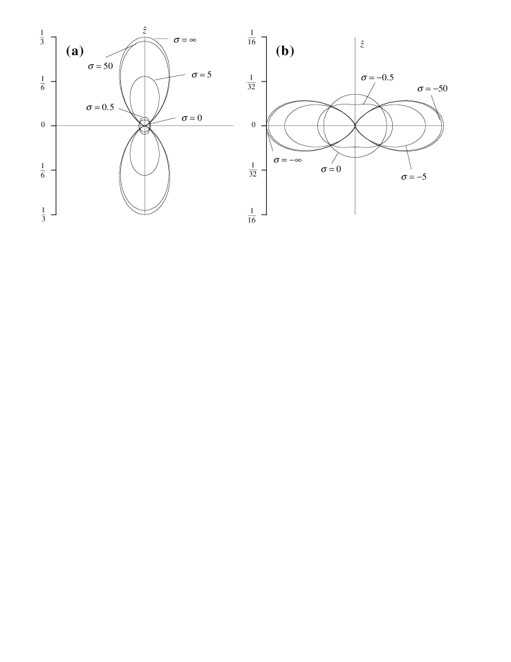
FIGURE 15.: Polar plots showing the angular dependence of the reduced non-linear susceptibility $-\chi_{3}^{{\rm red}}$ [Eq. (3.97)] for various values of the dimensionless anisotropy parameter $\sigma=Kv/k_{{\rm B}}T$. (a) Easy-axis anisotropy. (b) Easy-plane anisotropy.

The upper panel of Fig. 16 shows $\chi_{3}^{{\rm red}}$ vs. $\sigma$ in the longitudinal and transverse field cases, as well as for anisotropy axes distributed at random.

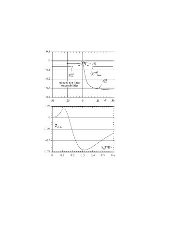
FIGURE 16.: Upper panel: Reduced non-linear susceptibility (3.97) in the longitudinal, $\chi_{3,\|}^{{\rm red}}$, and transverse, $\chi_{3,\perp}^{{\rm red}}$, field cases, and for anisotropy axes distributed at random, $\langle\chi_{3}^{{\rm red}}\rangle_{{\rm ran}}$, vs. the dimensionless anisotropy parameter $\sigma=Kv/k_{{\rm B}}T$. Lower panel: Temperature dependence of the transverse component of the non-linear susceptibility [from Eq. (3.93)]. $\chi_{3,\perp}$ is measured in units of $m(\mu_{0}/B_{K})^{3}$

The three curves coincide at $\sigma=0$, where the orientation of the magnetic field plays no rôle, taking the Langevin value $-1/45$. It is noticeable the large variation of $\chi_{3}^{{\rm red}}$ with respect to $\sigma$ for anisotropy axes parallel to the field. Note also that, although dramatically reduced, the anisotropy-induced temperature dependence of $\chi_{3}$ is kept for anisotropy axes distributed at random. On the other hand, we can again remark that, qualitatively, the longitudinal and the transverse field cases interchange their rôles when the sign of the anisotropy is reversed (see also Fig. 15). For instance, for easy-plane anisotropy $\chi_{3,\|}$ rapidly vanishes as $|\sigma|$ departs from zero. The analogous result for easy-axis anisotropy occurs in the presence of a transverse field; then $\chi_{3,\perp}$ rapidly decreases as $\sigma$ departs from zero. However, in this case $\chi_{3}$ does not exactly vanish, but it goes to a finite non-zero value for large $\sigma$ (which is not resolved with the scale used in Fig. 16). This will be discussed below.

c. The sign of the non-linear susceptibility.

As the non-linear susceptibility is a measure of the departure of the magnetization from the linear regime, and this departure usually consists of a bending downwards, one is tempted to conclude that $\chi_{3}$ is a negative quantity. Indeed, the above formula for anisotropy axes distributed at random [Eq. (3.96)] clearly shows that this is indeed the case for $\langle\chi_{3}\rangle_{{\rm ran}}$ (in accordance with the downward bending of the corresponding magnetization in Fig. 11). However, this result is not general as will be illustrated now with $\chi_{3,\perp}$. Let us compute the low temperature ($\sigma\gg 1$) expression for $\chi_{3,\perp}$ by using the asymptotic methods of Appendix A:

$$\chi_{3,\perp}=\frac{1}{16}\frac{\mu_{0}^{3}m^{4}}{(k_{{\rm B}}T)^{3}}\bigg{[}-1+2\frac{R^{\prime}}{R}-2\bigg{(}\frac{R^{\prime}}{R}\bigg{)}^{2}+\frac{R^{\prime\prime}}{R}\bigg{]}\simeq\frac{1}{16}\frac{\mu_{0}^{3}m^{4}}{(k_{{\rm B}}T)^{3}}\frac{1}{\sigma^{4}}\;,$$

so that

$$\chi_{3,\perp}\simeq\frac{1}{2}m\Big{(}\frac{\mu_{0}}{B_{K}}\Big{)}^{3}\,\frac{k_{{\rm B}}T}{Kv}\;.$$ (3.98)

Therefore, we see that, not only is $\chi_{3,\perp}$ positive at low temperatures, but it indeed increases linearly with $T$. At higher temperatures the above expansion must break down and the corresponding corrections bring $\chi_{3,\perp}$ to the negative values that it must take at sufficiently high temperatures ($\chi_{3,\perp}|_{\sigma\ll 1}\simeq\chi_{3,{\rm Lan}}=-[\mu_{0}^{3}m^{4}/45(k_{{\rm B}}T)^{3}]$). Thus, from the knowledge of the limit temperature dependences ($\chi_{3,\perp}\propto T$ and $-1/T^{3}$) one concludes that $\chi_{3,\perp}$ must have two peaks and cross the temperature axis at a certain intermediate temperature. This is precisely what it can be seen in the lower panel of Fig. 16, showing that $\chi_{3}\leq 0$ is not a general result. As $T$ decreases, $\chi_{3,\perp}$ has a negative minimum, increases, crosses zero, exhibits a secondary positive maximum, and eventually tends to zero at low temperatures. These are the typical features exhibited by the dynamical non-linear susceptibility $\chi_{3}(\omega,T)$ (Raĭkher and Stepanov, 1997), but their occurrence in the equilibrium susceptibility is somewhat unexpected. This is another good example of the effects of the magnetic anisotropy on the properties of superparamagnetic systems.

3. Generalizations

One can also derive the non-linear susceptibility by means of the relation between the thermal-equilibrium fluctuations of $\vec{m}$, in the absence of a probing field, and the actual magnetic response of the system, by-passing the explicit expansion of the magnetization in a series of powers of the field.

On inspecting the definition (3.41), one realizes that $\chi_{3}$ can be obtained by differentiating the magnetization as $\chi_{3}=\frac{1}{6}\mu_{0}^{3}\partial^{3}\big{\langle}\vec{m}\cdot\hat{b}\big{\rangle}_{{\rm e}}/\partial B^{3}|_{B=0}$. This is directly generalized to

$$\chi_{3}=\frac{1}{6}\mu_{0}^{3}\left.\frac{\partial^{3}\big{\langle}\vec{m}\cdot\hat{b}\big{\rangle}}{\partial(\Delta B)^{3}}\right|_{\Delta B=0}\;,$$ (3.99)

where $\Delta\vec{B}=\Delta B\,\hat{b}$ is an external probing field and the averages are now taken with respect to the total energy of the system in the presence of $\Delta\vec{B}$.

On calculating the above third-order derivative by making repeated use of the Eq. (3.58), one arrives at the general result [cf. Eq. (3.60)]

$$\chi_{3}=\frac{\mu_{0}^{3}}{(k_{{\rm B}}T)^{3}}\frac{1}{6} \Big{[} \big{\langle}(\vec{m}\cdot\hat{b})^{4}\big{\rangle}_{{\rm e}}-4\big{\langle}(\vec{m}\cdot\hat{b})^{3}\big{\rangle}_{{\rm e}}\big{\langle}\vec{m}\cdot\hat{b}\big{\rangle}_{{\rm e}}-3\big{\langle}(\vec{m}\cdot\hat{b})^{2}\big{\rangle}_{{\rm e}}^{2}$$

$${}+12\big{\langle}(\vec{m}\cdot\hat{b})^{2}\big{\rangle}_{{\rm e}}\big{\langle}\vec{m}\cdot\hat{b}\big{\rangle}_{{\rm e}}^{2}-6\big{\langle}\vec{m}\cdot\hat{b}\big{\rangle}_{{\rm e}}^{4}\Big{]}\;,$$

where the averages are finally taken in the absence of the probing field. Note however that if a bias field is applied, there is also a non-zero term in $(\Delta B)^{2}$, which defines the corresponding susceptibility $\chi_{2}$ (see, for example, Raĭkher et al., 1997). Nevertheless, on assuming that no constant field is applied and noting that, consequently, the above averages at zero probing field are then zero-field averages, we can use $\langle(\vec{m}\cdot\hat{b})^{2n+1}\rangle_{{\rm e}}|_{B=0}=0$, to get

$$\chi_{3}=\frac{\mu_{0}^{3}}{(k_{{\rm B}}T)^{3}}\frac{1}{6}\left.\left[\big{\langle}(\vec{m}\cdot\hat{b})^{4}\big{\rangle}_{{\rm e}}-3\big{\langle}(\vec{m}\cdot\hat{b})^{2}\big{\rangle}_{{\rm e}}^{2}\right]\right|_{B=0}\;.$$ (3.100)

This relation between the non-linear susceptibility and the thermal-equilibrium fluctuations of the magnetic moment in zero field, is valid for any form of the magnetic-anisotropy energy provided that this has inversion symmetry $\langle(\vec{m}\cdot\hat{b})^{2n+1}\rangle_{{\rm e}}=0$.

Finally, on returning to the simplest uniaxial-anisotropy case and recalling that the zero-field averages of $(\vec{m}\cdot\hat{b})^{2i}$ are directly related with the coefficients $C_{i}$ by Eq. (2.42), specifically

$$\big{\langle}(\vec{m}\cdot\hat{b})^{2}\big{\rangle}_{{\rm e}}\big{|}_{B=0}=m^{2}2C_{1}\;,\qquad\big{\langle}(\vec{m}\cdot\hat{b})^{4}\big{\rangle}_{{\rm e}}\big{|}_{B=0}=m^{4}12C_{2}\;,$$

one gets

$$\frac{1}{6}\left.\left[\big{\langle}(\vec{m}\cdot\hat{b})^{4}\big{\rangle}_{{\rm e}}-3\big{\langle}(\vec{m}\cdot\hat{b})^{2}\big{\rangle}_{{\rm e}}^{2}\right]\right|_{B=0}=m^{4}2\left(C_{2}-C_{1}^{2}\right)\;,$$

so that the expression (3.88) for $\chi_{3}$ is reobtained.

4. Approximate formulae for the non-linear susceptibility

We shall now derive approximate expressions for $\chi_{3}$, with the aim of establish simple approximate expressions valid in wide temperature ranges. Again, in order to obtain the approximate formulae we shall use the corresponding expressions for $R^{\prime}/R$ and $R^{\prime\prime}/R$ derived in Appendix A. (We could also proceed from the weak- and strong-anisotropy formulae for $M_{B}$.) The approximate expressions for the combinations of the functions $R^{(\ell)}/R$ entering in the general formula (3.93) are given by Eqs. (a), (b), and (b).

a. Weak-anisotropy range.

To obtain an approximate formula for $\chi_{3}$ valid for weak anisotropy, we insert Eqs. (a) into Eq. (3.93), gather the terms with the same power of $\sigma$, and express the trigonometric factors in terms of $\cos^{2}\!\alpha$ and $\cos^{4}\!\alpha$ only, obtaining

$$\left.\chi_{3}\right|_{|\sigma|\ll 1}\simeq-\frac{\mu_{0}^{3}m^{4}}{45(k_{{\rm B}}T)^{3}} \bigg{[} 1+\frac{8}{21}(3\cos^{2}\!\alpha-1)\sigma$$

$${}+\frac{8}{105}(4\cos^{4}\!\alpha-\cos^{2}\!\alpha)\sigma^{2}$$

$${}+\frac{32}{10395}(21\cos^{4}\!\alpha-18\cos^{2}\!\alpha+4)\sigma^{3}\bigg{]}\;.$$

This equation is a good approximation of the exact $\chi_{3}$ for $|\sigma|\leq 2$. Note that, in contrast to $\chi$, only the first correction to the leading (isotropic) result vanishes when the anisotropy axes are distributed at random [recall Eq. (3.37)].

b. Strong-anisotropy ranges.

Let us first consider the $\sigma\ll-1$ range. If we insert Eqs. (b) into Eq. (3.93) and gather the terms with the same power of $1/\sigma$, we obtain

$$\left.\chi_{3}\right|_{\sigma\ll-1}\simeq-\frac{\mu_{0}^{3}m^{4}\sin^{4}\!\alpha}{16(k_{{\rm B}}T)^{3}}\left[1+\frac{1}{\sigma}+(16\cot^{2}\alpha-1)\frac{1}{4\sigma^{2}}\right]\;.$$ (3.102)

This the desired approximate formula for $\chi_{3}$ valid in extreme easy-plane range. An approximate expression for $\sigma\gg 1$ can be obtained in a similar way. On inserting Eqs. (b) into Eq. (3.93) and gathering the terms with the same power of $1/\sigma$, we arrive at

$$\left.\chi_{3}\right|_{\sigma\gg 1}\simeq-\frac{\mu_{0}^{3}m^{4}\cos^{4}\!\alpha}{3(k_{{\rm B}}T)^{3}}\left[1-\frac{2}{\sigma}+(3\tan^{2}\alpha-1)\frac{1}{2\sigma^{2}}+(3\tan^{2}\alpha-4)\frac{1}{2\sigma^{3}}\right]\;.$$ (3.103)

These strong-anisotropy equations match the corresponding exact results for $|\sigma|\geq 5$. In fact, with the combined use of Eqs. (a.), (3.102), and (3.103), one can almost cover the exact $\chi_{3}$ in the whole temperature range. Again this arises directly from the reasonable patching shown in Appendix A of the exact $R^{\prime}/R$ and $R^{\prime\prime}/R$ curves yielded by the approximate formulae employed.

5. Temperature dependence of the non-linear susceptibility

a. Theoretical results.

We shall now study in more detail the temperature dependence of $\chi_{3}$. Facing the subsequent particularization of the results to a number of systems of magnetic nanoparticles, we shall consider the occurrence of a distribution of particle volumes. We shall however take the anisotropy constant $K$ and the spontaneous magnetization $M_{s}=m/v$ as fixed, i.e., neither distribution in particle shape, nor size effects on $M_{s}$ or $K$ will be considered. Then, if the anisotropy axes of the particles with the same volume are distributed at random, one can write

$$\chi_{3}=\int_{0}^{\infty}\!\!{\rm d}{v}\,v^{-1}\left\langle\chi_{3}\right\rangle_{{\rm ran}}f(v)\;,$$

where the factor $v^{-1}$ occurs since $f(v){\rm d}v$ is taken as the fraction of the total volume occupied by particles with volumes in the interval $(v,v+{\rm d}v)$.

In order to isolate the effect of the magnetic anisotropy on $\chi_{3}(T)$, we shall assume that $M_{s}$ is independent of $T$. This condition, which is obeyed at temperatures well below the ordering temperature of the magnetic material constituting the particles, yields also temperature independent anisotropy constants [this is apparent when the anisotropy is due to the magnetostatic self-energy, see Eq. (2.5)]. The computed quantity will be the dimensionless $\tilde{\chi}_{3}=\chi_{3}[K^{3}/(\mu_{0}^{3}M_{s}^{4})]$ and we shall employ a logarithmic-normal distribution for $f(v)$, namely

$$f(v)=\frac{1}{\sqrt{2\pi}\,\rho_{v}v}\exp\bigg{\{}-\frac{\left[\ln(v/v_{{\rm m}})\right]^{2}}{2\rho_{v}^{2}}\bigg{\}}\;,$$

where $v_{{\rm m}}$ is the median of the distribution and $\rho_{v}$ is the standard deviation of $\ln(v)$.

Figure 17 displays $\chi_{3}$ and the corresponding Ising and isotropic results vs. the temperature.

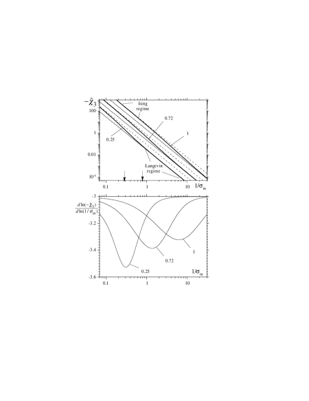
FIGURE 17.: Upper panel: Log-log plot of $-\tilde{\chi}_{3}$ vs. $1/\sigma_{{\rm m}}$ ($=k_{{\rm B}}T/Kv_{{\rm m}}$) for a system with randomly distributed anisotropy axes. The straight lines correspond to the isotropic (thin solid) and Ising (dashed) non-linear susceptibilities. The numbers mark the width $\rho_{v}$ of the volume distribution. The mean slope of the $\rho_{v}=0.72$ curve between the arrows is compared with the experiment of Bitoh et al. (1993) in the text. Lower panel: Logarithmic slopes.

As the influence of the anisotropy decreases with increasing $T$, $\chi_{3}$ undergoes a smooth crossover from the low-temperature Ising regime to the high-temperature isotropic regime. For $\sigma_{{\rm m}}\gg 1$ ($\sigma_{{\rm m}}=Kv_{{\rm m}}/k_{{\rm B}}T$) and $|\sigma_{{\rm m}}|\ll 1$, the logarithmic slope ${\rm d}\ln(-\chi_{3})/{\rm d}\ln(1/\sigma_{{\rm m}})$ tends to $-3$, indicating the limit $T^{-3}$ dependences. However, logarithmic slopes lesser than $-3$ emerge in the transitional regime, where the departure of $\chi_{3}(T)$ from an inverse-temperature-cubed law is sizable. As the width of the volume distribution increases, the crossover region widens and shifts to higher temperatures. This is due to the fact that the function $v^{3}f(v)$, which determines the particles making the most substantial contribution to $\chi_{3}$, broadens and moves to larger volumes, the $\chi_{3}$ of which is of Ising type over a wider interval of the displayed temperature range.

The rate of change of $\chi_{3}(T)$, moreover, increases as the anisotropy axes are aligned towards $\vec{B}$ (see Fig. 18).

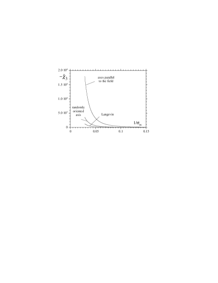
FIGURE 18.: Effect of the alignment of the anisotropy axes towards $\vec{B}$ on the temperature dependence of the non-linear susceptibility. The width of the volume distribution is $\rho_{v}=0.25$.

To illustrate, for a volume distribution with $\rho_{v}=0.25$, the maximum logarithmic slope changes from $-3.53$ for anisotropy axes distributed at random (see the lower panel of Fig. 17) to $-3.98$ for axes collinear with the field. On the other hand, although less dramatic, the discussed effects also occur for easy-plane anisotropy ($K<0$), being then magnified as $\vec{B}$ points towards the easy plane. Considering these significant deviations of $\chi_{3}(T)$ from a $T^{-3}$ dependence, arguments discarding superparamagnetism based on this type of departure, such as those employed by Schiffer et al. (1995), should be carefully scrutinized.

On the other hand, when observed over limited temperature windows (e.g., those imposed by the unavoidably finite measurement time), an increase of the equilibrium $\chi_{3}(T)$ steeper than $T^{-3}$ could resemble the high-temperature range of a quantity with a low-temperature divergence. This might misleadingly suggest the presence of appreciable inter-particle interactions in the ensemble and, consequently, one could try a fit of the non-linear susceptibility to, for example $\chi_{3}(T)\propto(T-T_{c})^{-3}$, obtaining false “critical” temperatures. If we do so with the $\chi_{3}(T)$ theoretically computed for the most diluted sample of Jonsson et al. (1995) over $100$ K $\leq T\leq 180$ K, we get the sizable value $T_{c}\simeq 17.3$ K (regression of the fit $0.99992$). Note that, for $\omega/2\pi\sim 1$–$10^{3}$ Hz, effects associated with the finite measurement time appear at $T\,\raisebox{1.50696pt}{$<$}\raisebox{-2.79857pt}{$\sim$}\,40$–$100$ K, below of which one cannot measure the equilibrium $\chi_{3}$.

b. Comparison with experimental data.

Bitoh et al. (1993; 1995) measured the non-linear dynamical susceptibility, $\chi_{3}(\omega,T)$, for cobalt particles precipitated in a Cu₉₇Co₃ alloy. From the equilibrium (high-temperature) part of the $\chi_{3}$ vs. $T$ curve they obtained a mean logarithmic slope $-3.17$, whose departure from $-3$ was not considered.

Their sample appears suitable to check the studied deviation of $\chi_{3}$ from a $T^{-3}$ law, since:

1. The high Curie temperature of the particles ($\simeq 1400$ K) yields $M_{s}$ feebly dependent on $T$ in the range of the experiment ($\leq 280$ K).

2. The equilibrium linear susceptibility can be fitted to a Curie law with a mean logarithmic slope $\langle{\rm d}\ln\chi/{\rm d}\ln T\rangle=-1.01$, compatible with the absence of dipole-dipole interaction effects and anisotropy axes distributed at random.

On the other hand, one can still argue that, due to finite size effects, the temperature dependence of the spontaneous magnetization of the Co particles could be larger than that of the bulk material, so that the measured temperature dependence of $\chi_{3}$ could be attributed to such phenomenon. However, the ascription of the extra $T^{-0.17}$ factor in $\chi_{3}(T)$ to $M_{s}(T)^{4}$, entails the occurrence of its square root in the Curie law [$\chi\propto M_{s}(T)^{2}$], yielding a total exponent $-(1+0.17/2)=-1.085$ for $\chi$, which is not consistent with the measured one ($-1.01$).

Unfortunately, the high amplitude of the oscillating field employed in their experiment ($v_{{\rm m}}M_{s}\Delta B/k_{{\rm B}}\simeq 17$ K) might have induced non-linear “saturation” effects on the measured susceptibilities at low temperatures, moving the volume distribution $f(v)$ that they derived from the $\chi(\omega,T)$ data, from the actual one. Even so, we have specialized the above calculation of $\chi_{3}(T)$ to the so-derived logarithmic-normal $f(v)$. The temperature range of their experiment, in the dimensionless units $k_{{\rm B}}T/Kv_{{\rm m}}$, is delimited in Fig. 17 by the arrows. Our calculation yields a mean logarithmic slope $-3.25$ that is within $2.5$% of the experimentally determined value $-3.17$. One must anyway conclude that the sizable departure of the theoretical exponent from $-3$, makes mandatory the inclusion of anisotropy effects on the temperature dependence of $\chi_{3}$ to achieve a complete understanding of this kind of experiments.

c. Proposed experiments.

In addition to search for deviations of $\chi_{3}(T)$ from a $T^{-3}$ law, the dependence of $\chi_{3}$ on the angle between the anisotropy axis and the applied field could be measured in systems with oriented anisotropy axes. (Molecular magnetic clusters and textured frozen magnetic fluids are examples of systems with parallel axes where such experiments could be performed.) In a polar plot (see Fig. 15), $\chi_{3}(\alpha)$ will undergo an increasing deformation from a circle at high temperatures (isotropic $\chi_{3}$) towards the characteristic two-looped shape of the Ising regime ($\chi_{3}|_{{\rm Ising}}\propto\cos^{4}\!\alpha$) as $T$ decreases.

Other possible experiment could be to measure $\chi_{3}(T)$ in a magnetic fluid through the freezing point of the solvent, $T_{{\rm f}}$. Recall that, due to the physical rotation of the particles in the fluid state, the magnetization is given by the Langevin law for each particle, irrespective of the anisotropy energy (Krueger, 1979). On the other hand, at temperatures below the freezing point, the anisotropy axes become immobilized; the magnetic anisotropy then takes reflection in the equilibrium quantities and $\chi_{3}(T)$ would undergo a discontinuous change at $T_{{\rm f}}$. In contrast, if at $T_{{\rm f}}$ the anisotropy axes become immobilized in a random pattern, the linear equilibrium susceptibility would be continuous there (recall that $\left\langle\chi\right\rangle_{{\rm ran}}$ does not depend on the anisotropy energy in a solid dispersion).

The relative size of the discontinuity in the non-linear susceptibility $\Delta\chi_{3}/\chi_{3}$ at the freezing temperature is determined by the value of $T_{{\rm f}}$ in magnetic-anisotropy units, so that the size of the jump also depends on the anisotropy constants and the actual volume distribution. We have computed $\Delta\chi_{3}/\chi_{3}$ with the parameters of two magnetic fluids in the literature. First, for most diluted sample of Luo et al. (1991), $\Delta\chi_{3}/\chi_{3}$ would be small, because the freezing point of the carrier liquid is close to the isotropic regime. On the other hand, for the most diluted sample of Jonsson et al. (1995), $\Delta\chi_{3}/\chi_{3}$ would be about $90$%. Once more, if the anisotropy axes are frozen collinear with $\vec{B}$, this effect will be even more dramatic.

IV Dynamical properties: heuristic approach

IV.A Introduction

In this Section we shall briefly consider a heuristic approach to the dynamics of classical magnetic moments in anisotropy potentials. We shall focus on the linear dynamical response, i.e., the response of the system to a small-amplitude, oscillating or constant, magnetic field. The responses to both types of stimulus are related in a simple way, so that we shall merely employ the language of the linear dynamical response in the frequency domain—the linear dynamical susceptibility $\chi(\omega)$. This quantity, in addition to supplying valuable information about the intrinsic dynamics of the spins, is of relevance for general studies on magnetic nanoparticle systems. For instance, under certain conditions $\chi(\omega)$ can be used to approximately determine the distribution of energy barriers (essentially particle volumes), occurring in assemblies of non-interacting magnetic nanoparticles (Shliomis and Stepanov, 1994). Besides, a rough estimate of the pre-exponential factor of the longitudinal relaxation time in the Arrhenius regime can also be derived from the $\chi(\omega)$ data.

The organization of this Section is as follows. In Subsec. IV.B various heuristic expressions that have been proposed to describe the linear dynamical response are discussed (they will be compared with exact numerical results in Section V). In Subsec. IV.C, the most general of those expressions will be analyzed in detail, illustrating how it can be used to get the energy-barrier distribution of magnetic nanoparticle ensembles. Finally, in Subsec. IV.D some of the previous results will be illustrated with experiments performed on a frozen magnetic fluid of maghemite ($\gamma$–Fe₂O₃) nanoparticles. Part of the results of this Section were presented by Svedlindh, Jonsson and García-Palacios (1997).

IV.B Heuristic treatment of the linear dynamical response

Let us commence by considering the expression (3.54) for the linear equilibrium susceptibility in terms of its longitudinal and transverse contributions, namely

$$\chi=\chi_{\|}\cos^{2}\!\alpha+\chi_{\perp}\sin^{2}\!\alpha\;,$$ (4.1)

where $\alpha$ is the angle between the anisotropy axis and the probing field. The term $\chi_{\|}\cos^{2}\!\alpha$ is proportional to the projection along the probing field direction of the response of the magnetic moment to the longitudinal component (with respect to the anisotropy axis) of the field. Likewise, $\chi_{\perp}\sin^{2}\!\alpha$ is proportional to the projection onto the probing field of the response of the spin to the transverse component of the field. As we know from Subsec. III.D, averaging this equation with $\chi_{\|}$ and $\chi_{\perp}$ from Eq. (3.53), one gets $\langle\chi\rangle_{{\rm ran}}=\mu_{0}m^{2}/3k_{{\rm B}}T$. Consequently, in a non-interacting magnetic nanoparticle ensemble with anisotropy axes distributed at random, the linear equilibrium susceptibility in the absence of an external bias field is independent of the magnetic anisotropy ($\chi$ is then identical with that derived in a naïve superparamagnetic model where the anisotropy is neglected). The main effect of the anisotropy is to introduce energy barriers that the spins need to overcome before equilibrium is reached, implying that the ensemble could, depending on the measurement time, display magnetic relaxation.

The relaxational mechanism consists of an orientational redistribution of the magnetic moments according to the conditions set by the magnetic anisotropy, temperature, and external field. The relaxation can be envisaged as a two-stage process: first, the dipoles redistribute inside the potential wells, with a characteristic time $\tau_{\perp}$ related with the inverse of the precession frequency of the magnetic moments in the anisotropy field ($\sim 10^{-10}$–$10^{-12}$ s); then, the equilibration between the potential wells, which is a thermally activated process, proceeds. This second mechanism can result in exceedingly slow magnetic relaxation since its characteristic time $\tau_{\|}$, which essentially follows an Arrhenius law [see Eq. (2.1)], ranges from picoseconds to geological time scales depending on the magnetic anisotropy, temperature, and external field.

A rigorous theoretical derivation of the linear dynamical susceptibility of classical magnetic moments in anisotropy potentials, as well as other dynamical quantities, is hindered by a number of mathematical difficulties (see Section V). Thus, in order to describe the linear dynamical response of non-interacting magnetic nanoparticles, various simple expressions have been proposed in the literature. We shall mainly consider the expression suggested, on the basis of the two-stage relaxation process mentioned, by Shliomis and Stepanov (1993) to describe $\chi(\omega)$ at frequencies below the ferromagnetic-resonance frequency range. Besides, we shall show that this model contains as particular cases some models previously proposed.

Shliomis and Stepanov model

In a study of magnetic fluids these authors suggested that $\chi(\omega)$ could be described as a sum of two independent Debye-type relaxation mechanisms: one for the response to the longitudinal component of the probing field and the other for the response to the transverse component (see also Raĭkher and Stepanov, 1997). The expression proposed can be generalized in order to describe the effect of a longitudinal bias field by merely writing

$$\chi_{{\rm ShS}}=\frac{\chi_{\|}(T,B)}{1+i\omega\tau_{\|}}\cos^{2}\!\alpha+\frac{\chi_{\perp}(T,B)}{1+i\omega\tau_{\perp}}\sin^{2}\!\alpha\;,$$ (4.2)

where $\chi_{\|}$ and $\chi_{\perp}$ are the exact equilibrium susceptibilities (3.70).

Various expressions can be used for the characteristic times appearing in the above formula (see Subsec. V.C). However, for the purposes of this Section it is sufficient to consider that in the high-barrier range $\tau_{\|}$ can be written in the Arrhenius form $\tau_{\|}=\tau_{0}\exp(\Delta U/k_{{\rm B}}T)$, where $\tau_{0}$ is assumed to be a constant $\sim 10^{-10}$–$10^{-12}$ s (that is, we disregard the dependences of the pre-exponential factor on the temperature, external field, and the parameters of the particles in comparison with the dependences of the exponential term). Concerning the transverse relaxation time, for not very high frequencies (say, $\omega\,\raisebox{1.50696pt}{$<$}\raisebox{-2.79857pt}{$\sim$}\,10^{6}$ Hz), the condition $\omega\tau_{\perp}\ll 1$ holds (Subsec. V.C). One can then approximate $1/(1+i\omega\tau_{\perp})$ by unity in Eq. (4.2), to get the low-frequency equation

$$\left.\chi_{\rm ShS}\right|_{\omega\tau_{\perp}\ll 1}\simeq\frac{\chi_{\|}}{1+i\omega\tau_{\|}}\cos^{2}\!\alpha+\chi_{\perp}\sin^{2}\!\alpha\;.$$ (4.3)

The approximation used is equivalent to assume from the outset that the response to the transverse components of the probing field is instantaneous. In fact, very short measurement times, such as those obtained in neutron scattering or ferromagnetic resonance experiments, are required to probe the intra-potential-well dynamics (see Table I).

From now on Eq. (4.2) with the exact equilibrium susceptibilities, will be referred to as the Shliomis and Stepanov equation. Further, the formula obtained when in the low-frequency Eq. (4.3) one uses the high-barrier approximations (3.85) and (3.86) of the equilibrium susceptibilities, will be called the Gittleman, Abeles, and Bozowski (1974) equation, since it properly generalizes their formula to $B\neq 0$ and an arbitrary anisotropy-axis orientation. Indeed, on introducing Eqs. (3.85) and (3.86) evaluated at $B=0$ [that is, Eqs. (3.82)] into Eq. (4.3), one first gets

$$\chi_{{\rm GAB}}\simeq\bigg{[}\frac{\mu_{0}m^{2}}{k_{{\rm B}}T}\cos^{2}\!\alpha+\frac{\mu_{0}m^{2}}{Kv}\big{(}{\textstyle\frac{3}{2}}\sin^{2}\!\alpha-1\big{)}+i\omega\tau_{\|}\frac{\mu_{0}m^{2}}{2Kv}\sin^{2}\!\alpha\bigg{]}\frac{1}{1+i\omega\tau_{\|}}\;,$$ (4.4)

which, when averaged over an ensemble with randomly distributed anisotropy axes (the second term in the square brackets then vanishes), reduces to the equation proposed in by the authors mentioned. Finally, the expression obtained when one introduces the Ising-type Eqs. (3.87) into Eq. (4.2) [or Eq. (4.3)], namely

$$\chi_{{\rm Ising}}=\frac{\mu_{0}m^{2}}{k_{{\rm B}}T}\frac{1}{\cosh^{2}\xi}\frac{\cos^{2}\!\alpha}{1+i\omega\tau_{\|}}\;,$$ (4.5)

is called the discrete-orientation or Ising dynamical susceptibility.

IV.C Analysis of the low-frequency Shliomis and Stepanov model

We shall now analyze the low-frequency Eq. (4.3) for an ensemble of non-interacting magnetic nanoparticles where there exists a distribution in particle parameters.

If the distribution occurs mainly in one of the parameters, say, the volumes of the particles, and one assumes that the contribution of each particle to the linear susceptibility is given by an expression like the low-frequency (4.3), one can write the linear susceptibility of the ensemble as

$$\chi(\omega,T)=\frac{\mu_{0}M_{s}^{2}}{k_{{\rm B}}T}\frac{1}{K}\int_{0}^{\infty}\!\!{\rm d}{E}\,f(E)E\left[\frac{R^{\prime}}{R}\frac{\langle\cos^{2}\!\alpha\rangle}{1+i\omega\tau_{\|}}+\frac{R-R^{\prime}}{2R}\langle\sin^{2}\!\alpha\rangle\right]\;.$$ (4.6)

In this equation the functions $R^{(\ell)}$ are evaluated at $\sigma=E/k_{{\rm B}}T$, $E=Kv$ (with $K$ assumed equal for all particles) and $f(E){\rm d}E$ is the fraction of the total “magnetic” volume occupied by those particles with energy barriers in the interval $(E,E+{\rm d}E)$. Note that the square of the magnetic moment has been written in terms of the spontaneous magnetization $M_{s}$ as $m^{2}=M_{s}^{2}v^{2}$ and, since we are using the “occupied volume” representation of the distribution, one $v$ is already incorporated into $f(E)$.

In the above formula, the orientational averages are taken with respect to the particles in $(E,E+{\rm d}E)$ and could, in principle, depend on $E$. We shall not study this situation but merely consider that $\langle\cos^{2}\!\alpha\rangle$ and $\langle\sin^{2}\!\alpha\rangle$ are the same for each energy interval. One could also consider the cases where, due to finite size effects, $M_{s}$ and $K$ depend on $v$. Although this could be incorporated in the following considerations, we shall not take those dependences into account explicitly.

1. The out-of-phase linear dynamical susceptibility and the energy-barrier distribution

The out-of-phase component (imaginary part) of Eq. (4.6) reads

$$\chi^{\prime\prime}(\omega)=\frac{\mu_{0}M_{s}^{2}\langle\cos^{2}\!\alpha\rangle}{k_{{\rm B}}T}\frac{1}{K}\int_{0}^{\infty}\!\!{\rm d}{E}\,f(E)E\,\frac{R^{\prime}}{R}\frac{\omega\tau_{\|}}{1+(\omega\tau_{\|})^{2}}\;,$$ (4.7)

to which the response to the transverse components of the probing field (with respect to the different anisotropy axes) does not contribute due to the low-frequency assumption ($\omega\,\raisebox{1.50696pt}{$<$}\raisebox{-2.79857pt}{$\sim$}\,10^{6}$ Hz).

The term $\omega\tau_{\|}/[1+(\omega\tau_{\|})^{2}]$ in the integrand of Eq. (4.7), has a maximum at the energy barrier, $E_{{\rm b}}$, for which $\omega\tau_{\|}=1$ (see Fig. 19).

FIGURE 19.: Real and imaginary parts of the Debye factor $1/(1+i\omega\tau_{\|})$ vs. the energy-barrier height $E/k_{{\rm B}}T$. The relaxation time is given by the Arrhenius law $\tau_{\|}=\tau_{0}\exp(E/k_{{\rm B}}T)$.

On assuming a simple Arrhenius form for the relaxation time, $\tau_{\|}=\tau_{0}\exp(E/k_{{\rm B}}T)$, one finds $E_{{\rm b}}=-k_{{\rm B}}T\ln(\omega\tau_{0})$, which explicitly depends on the temperature and the frequency. Besides, due to the exponential dependence assumed for $\tau_{\|}$, it follows from the definition of $E_{{\rm b}}$ that: (i) $\tau_{\|}(E)\ll\tau_{\|}(E_{{\rm b}})=1/\omega$, if $E<E_{{\rm b}}$, whereas (ii) $\tau_{\|}(E)\gg\tau_{\|}(E_{{\rm b}})=1/\omega$, if $E>E_{{\rm b}}$. In virtue of these properties, and considering that $1/\omega$ is the measurement time in a dynamical experiment, $E_{{\rm b}}$ is called the blocking barrier (recall the considerations in Section I). Similarly, one can define the corresponding dimensionless blocking barrier $\sigma_{{\rm b}}=E_{{\rm b}}/k_{{\rm B}}T$, whence

$$E_{{\rm b}}=-k_{{\rm B}}T\ln(\omega\tau_{0})\;,\qquad\sigma_{{\rm b}}=-\ln(\omega\tau_{0})\;.$$ (4.8)

For these two quantities one has, by definition, $\omega\tau_{\|}=1$.

We shall not consider the finite height and width of the function $\omega\tau_{\|}/[1+(\omega\tau_{\|})^{2}]$, but we shall take this function as a (unnormalized) Dirac delta centered at $\sigma_{{\rm b}}$. This replacement works when the remainder terms in the integrand of the formula for $\chi^{\prime\prime}(\omega)$ (e.g., the energy-barrier distribution) change slowly enough in the interval about $\sigma_{{\rm b}}$ where $\omega\tau_{\|}/[1+(\omega\tau_{\|})^{2}]$ differs appreciably from zero. Concerning the term $R^{\prime}/R$, when $\sigma_{{\rm b}}\,\raisebox{1.50696pt}{$>$}\raisebox{-2.79857pt}{$\sim$}\,15$–$25$, its changes are not very large, because

$$\frac{{\rm d}{}}{{\rm d}\sigma}\bigg{(}\frac{R^{\prime}}{R}\bigg{)}=\frac{R^{\prime\prime}}{R}-\bigg{(}\frac{R^{\prime}}{R}\bigg{)}^{2}\stackrel{{\scriptstyle{\rm Eq.\ (\ref{comb:F:leadingterm})}}}{{\simeq}}\frac{1}{\sigma^{2}}\sim\frac{1}{400}\;,\quad\mbox{for}\quad\sigma\sim 20\;.$$

Values of $\sigma_{{\rm b}}\,\raisebox{1.50696pt}{$>$}\raisebox{-2.79857pt}{$\sim$}\,15$–$25$ are typical for probing fields with $\omega\,\raisebox{1.50696pt}{$<$}\raisebox{-2.79857pt}{$\sim$}\,10^{3}$ Hz.

Under the conditions mentioned, $\omega\tau_{\|}/[1+(\omega\tau_{\|})^{2}]$ plays the rôle of a function proportional to a Dirac delta. In order to calculate the proportionality factor, one integrates that function over the entire energy range by means of the substitution ${\rm d}\tau_{\|}=(\tau_{\|}/k_{{\rm B}}T){\rm d}E$

$$\int_{0}^{\infty}\!\!{\rm d}{E}\,\frac{\omega\tau_{\|}}{1+(\omega\tau_{\|})^{2}}=k_{{\rm B}}T\int_{\tau_{0}}^{\infty}\!\!{\rm d}{\tau_{\|}}\,\frac{\omega}{1+(\omega\tau_{\|})^{2}}\simeq\frac{\pi}{2}k_{{\rm B}}T\;,$$

where, on considering the low-frequency assumption ($\omega\,\raisebox{1.50696pt}{$<$}\raisebox{-2.79857pt}{$\sim$}\,10^{6}$ Hz) and taking the tiny value of $\tau_{0}$ ($\sim 10^{-10}$–$10^{-12}$ s) into account, we have used the approximation $\arctan(\omega\tau_{0})\,\raisebox{1.50696pt}{$<$}\raisebox{-2.79857pt}{$\sim$}\,\arctan(10^{-4}$–$10^{-6})\simeq 0$. Therefore, when integrating functions slowly varying about $E_{{\rm b}}=-k_{{\rm B}}T\ln(\omega\tau_{0})$, one can make use of the approximation

$$\frac{\omega\tau_{\|}}{1+(\omega\tau_{\|})^{2}}\simeq\frac{\pi}{2}k_{{\rm B}}T\,\delta(E-E_{{\rm b}})\;.$$ (4.9)

Thus, on calculating the integral in Eq. (4.7) by means of Eq. (4.9), one obtains (cf. Eq. (41) by Shliomis and Stepanov, 1994)

$$\chi^{\prime\prime}(\omega,T)=\frac{\pi}{2}\frac{\mu_{0}M_{s}^{2}}{K}\langle\cos^{2}\!\alpha\rangle\frac{R^{\prime}(\sigma_{{\rm b}})}{R(\sigma_{{\rm b}})}f(E_{{\rm b}})E_{{\rm b}}\;,$$ (4.10)

which directly relates the energy-barrier distribution and the out-of-phase linear dynamical susceptibility. Note that, even if we consider the weak temperature dependence of $\tau_{0}$, this is further weakened when occurring inside the logarithm $\ln(\omega\tau_{0})$, so that $\sigma_{{\rm b}}=-\ln(\omega\tau_{0})$ and thus the factor $R^{\prime}(\sigma_{{\rm b}})/R(\sigma_{{\rm b}})$, are almost independent of $T$. Then, because $R^{\prime}(\sigma_{{\rm b}})/R(\sigma_{{\rm b}})$ is also weakly dependent on $\omega$, Eq. (4.10) shows that, approximately, all the dependence of $\chi^{\prime\prime}$ on $T$ and $\omega$ enters via the combination $E_{{\rm b}}=-k_{{\rm B}}T\ln(\omega\tau_{0})$. Therefore, if we plot $\chi^{\prime\prime}$ vs. $-k_{{\rm B}}T\ln(\omega\tau_{0})$, all the $\chi^{\prime\prime}(T)$ curves corresponding to different frequencies collapse onto a single “master” curve [proportional to $f(E)E$ and with maximum at $E_{{\rm M}}$]. Conversely, by fitting the frequency-dependent temperature of the maximum of $\chi^{\prime\prime}(T)$, denoted by $T_{{\rm M}}(\omega)$, to the “Arrhenius law” $E_{{\rm M}}=-k_{{\rm B}}T_{{\rm M}}(\omega)\ln(\omega\tau_{0})$, one can get $E_{{\rm M}}$ and $\tau_{0}$.

Note however that the parameter $E_{{\rm M}}$, which is sometimes called “average energy barrier”, is merely the maximum of the function $f(E)E$. Therefore, it is not necessarily related with a characteristic parameter of the energy-barrier distribution (incidentally, for the gamma and logarithmic-normal distributions $E_{{\rm M}}$ is equal to the mean and the median of the distribution, respectively).

2. The in-phase linear dynamical susceptibility

The in-phase component (real part) of Eq. (4.6) is given by

$$\chi^{\prime}=\frac{\mu_{0}M_{s}^{2}}{k_{{\rm B}}T}\frac{1}{K}\int_{0}^{\infty}\!\!{\rm d}{E}\,f(E)E\left[\frac{R^{\prime}}{R}\frac{\langle\cos^{2}\!\alpha\rangle}{1+(\omega\tau_{\|})^{2}}+\frac{R-R^{\prime}}{2R}\langle\sin^{2}\!\alpha\rangle\right]\;,$$ (4.11)

where, because of the low-frequency assumption ($\omega\,\raisebox{1.50696pt}{$<$}\raisebox{-2.79857pt}{$\sim$}\,10^{6}$ Hz), the response to the transverse components of the probing field contribute to $\chi^{\prime}(\omega)$ with its thermal-equilibrium value.

The term $1/[1+(\omega\tau_{\|})^{2}]$ as a function of $\sigma=E/k_{{\rm B}}T$ has the form of a smooth step about $\sigma_{{\rm b}}$, whose width is of the order of the width of the peak of $\omega\tau_{\|}/[1+(\omega\tau_{\|})^{2}]$ (see Fig. 19). However, when that term is under the integral sign and multiplied by functions that vary slowly around $\sigma_{{\rm b}}$, we can approximate $1/[1+(\omega\tau_{\|})^{2}]$ by a step function, namely

$$\frac{1}{1+(\omega\tau_{\|})^{2}}\simeq\left\{\begin{array}[]{ll}1&\mbox{~{}for~{}}E<E_{{\rm b}}\\ 0&\mbox{~{}for~{}}E>E_{{\rm b}}\end{array}\right.\;.$$ (4.12)

Thus, on introducing Eq. (4.12) into Eq. (4.11) and rearranging the integration limits, one gets the approximate result

$$\chi^{\prime}(\omega) = \frac{\mu_{0}M_{s}^{2}}{k_{{\rm B}}T}\frac{1}{K}\int_{0}^{E_{{\rm b}}}\!\!{\rm d}{E}\,f(E)E\left[\frac{R^{\prime}}{R}\langle\cos^{2}\!\alpha\rangle+\frac{R-R^{\prime}}{2R}\langle\sin^{2}\!\alpha\rangle\right]$$ (4.13)

$${}+\frac{\mu_{0}M_{s}^{2}}{k_{{\rm B}}T}\frac{1}{K}\int_{E_{{\rm b}}}^{\infty}\!\!{\rm d}{E}\,f(E)E\,\frac{R-R^{\prime}}{2R}\langle\sin^{2}\!\alpha\rangle\;,$$

which can be interpreted as follows. Note first that only the particles with $E<E_{{\rm b}}$, i.e., those obeying $\tau_{\|}(E)\ll\tau_{\|}(E_{{\rm b}})=1/\omega$, contribute to the first term. However, $1/\omega$ is the measurement time in a dynamical experiment, so that those particles are the superparamagnetic particles ($\tau_{\|}\ll 1/\omega$), and the first term is indeed their contribution to the linear equilibrium susceptibility. On the other hand, the particles with $E>E_{{\rm b}}$, which are those contributing to the second term, satisfy $\tau_{\|}(E)\gg\tau_{\|}(E_{{\rm b}})=1/\omega$, so that the over-barrier rotation process is not effective for them. These are the blocked particles, and contribute to $\chi^{\prime}(\omega)$ via the fast rotations of their magnetic moments inside the potential wells towards the transverse components of the field. In fact, the second term in Eq. (4.13) is $\langle\sin^{2}\!\alpha\rangle$ times the equilibrium transverse susceptibility of the blocked particles.

We finally note that, since $E_{{\rm b}}=-k_{{\rm B}}T\ln(\omega\tau_{0})$, the second term in Eq. (4.13) is small in comparison with the first one at sufficiently high temperatures, so that $\chi^{\prime}$ is then approximately equal to the equilibrium susceptibility. In addition, for anisotropy axes distributed at random we can write

$$\left.\left\langle\chi^{\prime}\right\rangle_{{\rm ran}}\right|_{{\rm high~{}}T}=\frac{\mu_{0}M_{s}^{2}}{3k_{{\rm B}}T}\frac{1}{K}\int_{0}^{\infty}\!\!{\rm d}{E}\,f(E)E\equiv\frac{C}{T}\;,$$ (4.14)

where $C$ is the Curie constant.

3. The $\pi/2$-law

We shall now explicitly derive, starting from the low-frequency Shliomis and Stepanov equation (4.6), a celebrated relation between $\partial\chi^{\prime}/\partial\ln\omega$ and $\chi^{\prime\prime}$ known as the $\pi/2$-law.

First, on rearranging the integration limits in Eq. (4.13), we can write $\chi^{\prime}(\omega)$ as

$$\chi^{\prime}(\omega) = \frac{\mu_{0}M_{s}^{2}\langle\cos^{2}\!\alpha\rangle}{k_{{\rm B}}T}\frac{1}{K}\int_{0}^{E_{{\rm b}}}\!\!{\rm d}{E}\,f(E)E\frac{R^{\prime}}{R}$$ (4.15)

$${}+\frac{\mu_{0}M_{s}^{2}\langle\sin^{2}\!\alpha\rangle}{k_{{\rm B}}T}\frac{1}{K}\int_{0}^{\infty}\!\!{\rm d}{E}\,f(E)E\,\frac{R-R^{\prime}}{2R}\;,$$

where the last term, which is $\langle\sin^{2}\!\alpha\rangle$ times the transverse equilibrium susceptibility of the whole ensemble, does not depend on $\omega$. Then, on using $\partial E_{{\rm b}}/\partial\ln\omega=-k_{{\rm B}}T$ and the Leibniz formula

$$\frac{{\rm d}{}}{{\rm d}x}\int_{g(x)}^{h(x)}\!\!{\rm d}{t}\,F(x,t)=\left\{F[x,h(x)]h^{\prime}(x)-F[x,g(x)]g^{\prime}(x)\right\}+\int_{g(x)}^{h(x)}\!\!{\rm d}{t}\,\frac{\partial{}}{\partial x}F(x,t)\;.$$ (4.16)

one gets

$$\frac{\partial\chi^{\prime}}{\partial\ln\omega}=-\frac{\mu_{0}M_{s}^{2}}{K}\langle\cos^{2}\!\alpha\rangle\frac{R^{\prime}(\sigma_{{\rm b}})}{R(\sigma_{{\rm b}})}f(E_{{\rm b}})E_{{\rm b}}\;.$$ (4.17)

Finally, on comparing this equation with Eq. (4.10), we get the desired relation between $\partial\chi^{\prime}/\partial\ln\omega$ and $\chi^{\prime\prime}$, namely

$$\chi^{\prime\prime}=-\frac{\pi}{2}\frac{\partial\chi^{\prime}}{\partial\ln\omega}\;.$$ (4.18)

For systems with a sufficiently wide distribution of relaxation times, the $\pi/2$-law is in fact a quite general result and independent of the dynamical model used, since it can then be derived from the Kramers–Kronig relations. These relations are merely based on general principles as the linearity of the response, and causality (i.e., the response at time $t$ only depends on the values of the stimulus at times $t^{\prime}<t$). For the sake of completeness, we shall repeat here one such derivation of the $\pi/2$-law by Böttcher and Bordewijk (1978, p. 58).

On writing one of the Kramers–Kronig relations in the form

$$\chi^{\prime}(\omega)=\chi_{S}+\frac{2}{\pi}\int_{0}^{\infty}\!\!{\rm d}{\tilde{\omega}}\,\frac{\tilde{\omega}\chi^{\prime\prime}(\tilde{\omega})}{\tilde{\omega}^{2}-\omega^{2}}=\chi_{S}+\frac{2}{\pi}\int_{-\infty}^{\infty}\!\!{\rm d}{(\ln\tilde{\omega})}\,\frac{\tilde{\omega}^{2}\chi^{\prime\prime}(\tilde{\omega})}{\tilde{\omega}^{2}-\omega^{2}}\;,$$

where $\chi_{S}$ is the adiabatic ($\omega\to\infty$) susceptibility ($\chi_{\perp}$ in our case), and approximating in the last integral the factor $\tilde{\omega}^{2}/(\tilde{\omega}^{2}-\omega^{2})$ by a unit step function (with step at $\omega$), one obtains

$$\chi^{\prime}(\omega)\simeq\chi_{S}+\frac{2}{\pi}\int_{\ln\omega}^{\infty}\!\!{\rm d}{(\ln\tilde{\omega})}\,\chi^{\prime\prime}(\tilde{\omega})\;.$$

Then, on differentiating this equation with respect to $\ln\omega$ by means of the Leibniz formula (4.16) one finally gets the $\pi/2$-law.

The assumption of broad relaxation-time spectrum enters implicitly when approximating the factor $\tilde{\omega}^{2}/(\tilde{\omega}^{2}-\omega^{2})$ by a step function: the broad spectrum entails flat curves for $\chi^{\prime\prime}(\omega)$, so that the replacement mentioned does not introduce a significant error. This approximation is equivalent to the assumptions made above concerning the change of the functions appearing in the integrand of the equations for $\chi(\omega)$, in the range where the Debye factor has its maximum variation.

4. $\partial(T\chi^{\prime})/\partial T$ and its relation with $\chi^{\prime\prime}$ and the energy-barrier distribution

Wohlfarth (1979), when studying spin glasses in the context of the superparamagnetic cluster model, proposed a method to obtain the energy-barrier distribution from the derivative $\partial(T\chi^{\prime})/\partial T$. He considered a distribution of “blocking temperatures,” which in our notation are $T_{{\rm b}}=E_{{\rm b}}/k_{{\rm B}}$ (“blocking energies” in temperature units), and disregarded the contribution of the blocked clusters, and wrote

$$\chi(T)\simeq\frac{C}{T}\int_{0}^{T}\!\!{\rm d}{T_{{\rm b}}}\,f(T_{{\rm b}})\;.$$ (4.19)

Here $C$ is the Curie constant, and the susceptibility is the non-equilibrium susceptibility obtained in a dc experiment with a typical measurement time $\sim 100$ s. Then, by means of the inversion procedure [see Eq. (4.16)]

$$f(T)=\frac{1}{C}\frac{\partial(T\chi)}{\partial T}\;,$$ (4.20)

he expressed the distribution of blocking temperatures in terms of the linear susceptibility.

Note that Eq. (4.19) can be considered as the particular case of Eq. (4.13) where the anisotropy axes are distributed at random (the term in the square brackets in the first integral then equals $1/3$) and the second integral (the $\chi_{\perp}$ of the blocked clusters) is neglected (Ising-type case). Besides, in order to establish this correspondence we must assume that his $f(T_{{\rm b}})$ incorporates the extra energy factor, i.e., that $f(T_{{\rm b}})\propto Ef(E)$.

Lundgren, Svedlindh and Beckman (1981) derived a relation between $\chi^{\prime\prime}$ and $\partial(T\chi^{\prime})/\partial T$ for the following model

$$\chi(\omega)=\int_{\ln\tau_{{\rm min}}}^{\ln\tau_{{\rm max}}}\!\!{\rm d}{(\ln\tau)}\,g(\tau)\chi(\tau)\frac{1}{1+i\omega\tau}\;,$$ (4.21)

where $\chi(\tau)$ is the equilibrium susceptibility and $g(\tau)$ the distribution of relaxation times. They assumed $\chi(\tau)\propto 1/T$ and an Arrhenius dependence for $\tau$, getting

$$\chi^{\prime\prime}=-\frac{\pi}{2}\frac{1}{\ln(\omega\tau_{0})}\frac{\partial(T\chi^{\prime})}{\partial T}\;.$$ (4.22)

Because in the model (4.21), $\chi^{\prime\prime}$ is also directly related with the distribution of relaxation times, the above relation yields an inversion procedure analogous to that of Wohlfarth.

We shall now calculate $\partial(T\chi^{\prime})/\partial T$ for the low-frequency (4.6). In this way, we shall take into account the effect of the finite width and depth of the anisotropy potential wells.

Let us begin by taking the $T$-derivative of $T\chi^{\prime}$, with $\chi^{\prime}$ given by Eq. (4.13) [or Eq. (4.15)]. Since the integrals in those equations also depend on $T$ via the integration limits, the required $T$-derivative can be taken by dint of the Leibniz formula (4.16). On doing so, we get after the rearrangement of the integration limits,

$$\frac{\partial(T\chi^{\prime})}{\partial T} = -\ln(\omega\tau_{0})\frac{\mu_{0}M_{s}^{2}}{K}\langle\cos^{2}\!\alpha\rangle\frac{R^{\prime}(\sigma_{{\rm b}})}{R(\sigma_{{\rm b}})}f(E_{{\rm b}})E_{{\rm b}}$$

$${}+\frac{\mu_{0}M_{s}^{2}}{2K}\langle\sin^{2}\!\alpha\rangle\int_{E_{{\rm b}}}^{\infty}\!\!{\rm d}{E}\,f(E)\bigg{[}\frac{R^{\prime\prime}}{R}-\bigg{(}\frac{R^{\prime}}{R}\bigg{)}^{2}\bigg{]}\sigma^{2}$$

$${}+\frac{\mu_{0}M_{s}^{2}}{2K}\left[3\langle\cos^{2}\!\alpha\rangle-1\right]\int_{0}^{E_{{\rm b}}}\!\!{\rm d}{E}\,f(E)\bigg{[}\frac{R^{\prime\prime}}{R}-\bigg{(}\frac{R^{\prime}}{R}\bigg{)}^{2}\bigg{]}\sigma^{2}\;,$$

where we have assumed that neither $M_{s}$ nor $K$ depend on $T$, and used $\partial E_{{\rm b}}/\partial T=-k_{{\rm B}}\ln(\omega\tau_{0})$ as well as $(E/k_{{\rm B}})\partial\sigma/\partial T=-\sigma^{2}$.

Note that the first line on the right-hand side of Eq. (4.) is directly related with the energy-barrier distribution. If the remainder terms were absent, this equation would give the inversion procedure of Wohlfarth (4.20). However, since the last two lines contain information about $f(E)$ in integral form, we see that the quantity $\partial(T\chi^{\prime})/\partial T$ does not directly scan the energy-barrier distribution. Note in this connection that, unlike $\chi^{\prime\prime}$ (or $\partial\chi^{\prime}/\partial\ln\omega$) the quantity $[1/\ln(\omega\tau_{0})]\partial(T\chi^{\prime})/\partial T$ does not properly scale when represented against $-k_{{\rm B}}T\ln(\omega\tau_{0})$ due to the presence of the mentioned integral terms.

Next, on taking Eq. (4.10) into account we get the following relation between $\chi^{\prime\prime}$ and $\partial(T\chi^{\prime})/\partial T$

$$\chi^{\prime\prime}=-\frac{\pi}{2}\frac{1}{\ln(\omega\tau_{0})} \Bigg{\{} \frac{\partial(T\chi^{\prime})}{\partial T}-\frac{\mu_{0}M_{s}^{2}}{2K}\langle\sin^{2}\!\alpha\rangle\int_{E_{{\rm b}}}^{\infty}\!\!{\rm d}{E}\,f(E)\bigg{[}\frac{R^{\prime\prime}}{R}-\bigg{(}\frac{R^{\prime}}{R}\bigg{)}^{2}\bigg{]}\sigma^{2}$$

$${}-\frac{\mu_{0}M_{s}^{2}}{2K}\left[3\langle\cos^{2}\!\alpha\rangle-1\right]\int_{0}^{E_{{\rm b}}}\!\!{\rm d}{E}\,f(E)\bigg{[}\frac{R^{\prime\prime}}{R}-\bigg{(}\frac{R^{\prime}}{R}\bigg{)}^{2}\bigg{]}\sigma^{2}\Bigg{\}}\;,$$

which is the counterpart of Eq. (4.22) in the low-frequency Shliomis and Stepanov model. Furthermore, since the angular factor in the last term on the right-hand side vanishes for anisotropy axes distributed at random, the above relation simplifies in that case to

$$\left\langle\chi^{\prime\prime}\right\rangle_{{\rm ran}}=-\frac{\pi}{2}\frac{1}{\ln(\omega\tau_{0})}\Bigg{\{}\frac{\partial(T\left\langle\chi^{\prime}\right\rangle_{{\rm ran}})}{\partial T}-\frac{\mu_{0}M_{s}^{2}}{3K}\int_{E_{{\rm b}}}^{\infty}\!\!{\rm d}{E}\,f(E)\bigg{[}\frac{R^{\prime\prime}}{R}-\bigg{(}\frac{R^{\prime}}{R}\bigg{)}^{2}\bigg{]}\sigma^{2}\Bigg{\}}\;,$$ (4.24)

Finally, since $\sigma>\sigma_{{\rm b}}\sim 20$–$25$, if $E>E_{{\rm b}}$, one can replace $R^{\prime\prime}/R-(R^{\prime}/R)^{2}$ in the above integral by its high-barrier approximation (A.32), to get

$$\left\langle\chi^{\prime\prime}\right\rangle_{{\rm ran}}=-\frac{\pi}{2}\frac{1}{\ln(\omega\tau_{0})}\bigg{\{}\frac{\partial{}}{\partial T}(T\left\langle\chi^{\prime}\right\rangle_{{\rm ran}})-\frac{\mu_{0}M_{s}^{2}}{3K}\int_{E_{{\rm b}}}^{\infty}\!\!{\rm d}{E}\,f(E)\bigg{\}}\;.$$ (4.25)

This is an interesting result: in spite of the differences between $\chi^{\prime\prime}$ and $\partial(T\chi^{\prime})/\partial T$ being reduced upon averaging for anisotropy axes distributed at random, some of them remain. These differences, and accordingly those of $\partial(T\chi^{\prime})/\partial T$ with respect to the energy-barrier distribution, are again due to the presence of the second term on the right-hand side, which contains information about $f(E)$ in integral form. In addition, the lower the temperature, the larger the differences mentioned, because the lower integration limit in Eq. (4.25) decreases with $T$ (recall that $E_{{\rm b}}\propto k_{{\rm B}}T$).

Note finally that, by using the high-barrier formula $\chi_{\perp}\simeq\mu_{0}m^{2}/2Kv$ per particle [Eqs. (3.82)], the integral in Eq. (4.25) can alternatively be written in terms of the approximate transverse susceptibility of the blocked particles (at the temperature and frequency considered), namely

$$\left\langle\chi^{\prime\prime}\right\rangle_{{\rm ran}}=-\frac{\pi}{2}\frac{1}{\ln(\omega\tau_{0})}\left\{\frac{\partial{}}{\partial T}(T\left\langle\chi^{\prime}\right\rangle_{{\rm ran}})-\frac{2}{3}\chi_{\perp,{\rm blo}}\right\}\;.$$ (4.26)

Therefore, we find the $T$- and $\omega$-dependent criterion $(2/3)\chi_{\perp,{\rm blo}}\ll\partial(T\chi^{\prime})/\partial T$, for the quantity $\partial(T\chi^{\prime})/\partial T$ scanning the energy-barrier distribution as properly as $\chi^{\prime\prime}$ (for anisotropy axes distributed at random only). Recall that no restriction of this type exists for the obtainment of the energy-barrier distribution from $\chi^{\prime\prime}$ (or $\partial\chi^{\prime}/\partial\ln\omega$). Note also that, not only $\chi_{\perp,{\rm blo}}$ is the transverse susceptibility of the blocked particles but, when multiplied by $\langle\sin^{2}\!\alpha\rangle_{{\rm ran}}=2/3$, is their total contribution to the susceptibility, because the over-barrier relaxation mechanism is indeed “blocked” for those particles.

IV.D Comparison with experiment

To conclude, we shall briefly illustrate some of the results of the previous subsection with experiments performed on a frozen magnetic fluid containing nanometric maghemite ($\gamma$–Fe₂O₃) particles.

FIGURE 20.: Temperature dependence of the in-phase (upper panels) and out-of-phase (lower panels) components of the dynamical susceptibility of a frozen magnetic fluid of maghemite particles. Left panels: solid lines computed with the Ising-type model where $\chi_{\|}=\mu_{0}m^{2}/k_{{\rm B}}T$ and $\chi_{\perp}=0$ (per particle). Right panels: solid lines computed with the low-frequency Shliomis and Stepanov equation (4.6).

The degree of dilution of the sample studied was $\sim 0.03$% by volume, in order to avoid dipole-dipole interaction effects. This illustrates one of the advantages of the use of frozen magnetic fluids for fundamental studies on systems of magnetic nanoparticles: by simple dilution and subsequent freezing of the magnetic fluid, one can get a series of solid dispersions of nanoparticles where the strength of the interactions is tuned almost as desired. (This method also guarantees that all the samples have the same distribution in particle parameters.) Another advantage of these systems is that by means of the application of magnetic fields when freezing the samples, one can produce systems with different anisotropy-axis distributions. The sample considered here (Svedlindh et al., 1997) was frozen in zero field, so that a random distribution of the anisotropy axes is to be expected.

1. Comparison with the Ising-type and Shliomis and Stepanov models

Figure 20 displays the measured dynamical susceptibility and the Ising-type theoretical curves computed with the energy-barrier distribution derived from $\chi^{\prime\prime}$. While the calculated and experimental out-of-phase susceptibilities compare to a high degree of precision (by construction), the matching of the in-phase curves is comparatively poor. One may guess that the reason for this poor matching is the absence of the transverse response in the model employed. In order to check this hypothesis, Fig. 20 also displays the same experimental results together with the curves computed with the low-frequency Shliomis and Stepanov equation. One can see that the description of the experimental curves provided by this model has improved significantly.

FIGURE 21.: $\chi^{\prime\prime}(T)$ (open symbols) and $-[\pi/2\ln(\omega\tau_{0})]\partial(T\chi^{\prime})/\partial T$ (filled symbols) vs. $-T\ln(\omega\tau_{0})$ of a frozen magnetic fluid of maghemite particles at the frequency $\omega/2\pi=320$ Hz.

2. Comparison of $\chi^{\prime\prime}$ with $\partial(T\chi^{\prime})/\partial T$

Equation (4.24) suggests that a joint plot of $\chi^{\prime\prime}$ and $\partial(T\chi^{\prime})/\partial T$ could be an alternative means to show the necessity of including the transverse response of the nanoparticles. When this contribution to the total response is negligible, those two curves should trace out the same energy-barrier dependence, whereas one would expect $(\pi/2\sigma_{{\rm b}})\partial(T\chi^{\prime})/\partial T$ being larger than $\chi^{\prime\prime}$ otherwise. Moreover, one would also expect that, the lower the temperature, the larger the differences between the two curves, because the lower limit in the integral of Eq. (4.24) decreases with $T$. This is what is indeed observed in Fig. 21, giving further evidence of the necessity of including the transverse contribution to the total response of the studied magnetic nanoparticle system. The figure also confirms the point that $\partial(T\chi^{\prime})/\partial T$ does not determine the energy-barrier distribution as accurately as $\chi^{\prime\prime}$ does.

V Dynamical properties: stochastic approach

V.A Introduction

In this Section we shall study the dynamics of classical spins in the context of the theory of stochastic processes.

In order to study the properties of classical magnetic moments, numerical simulation techniques can also be used, with most of the studies that have been performed being based on the Monte Carlo method. Although this method is a rigorous and efficient tool to compute thermal-equilibrium quantities, the interpretation of the dynamical properties derived by means of Monte Carlo techniques, especially for non-Ising spins, is not free from criticism (Ettelaie and Moore, 1984; Binder and Stauffer, 1984). On the contrary, when using stochastic methods based on Fokker–Planck or Langevin equations, time does not merely label the sequential order of generated states when sampling the phase space, but is related with physical time.

For classical spins, the basic Langevin equation is the stochastic Landau–Lifshitz (–Gilbert) equation introduced by Brown (1963) (see also, Kubo and Hashitsume, 1970). The multiplicative fluctuating terms occurring in this Langevin equation were treated in Brown’s work, as well as in the subsequent theoretical developments, by means of the Stratonovich stochastic calculus. In this context, Brown constructed the celebrated Fokker–Planck (diffusion) equation for the time evolution of the non-equilibrium probability distribution of magnetic moment orientations.

In order to solve Brown’s Fokker–Planck equation (a partial differential equation of parabolic type) a number of techniques have been used, such as direct solution techniques (Rodé, Bertram and Fredkin, 1987) or more elaborate approaches involving continued-fractions techniques or the numerical calculation of the eigenvalues and amplitudes of the relevant dynamical modes (Aharoni, 1964; Bessais, Ben Jaffel and Dormann, 1992; Coffey, Crothers, Kalmykov, Massawe and Waldron, 1994; Raĭkher and Stepanov, 1995b; Coffey, Crothers, Kalmykov and Waldron, 1995a).

An approach equivalent to solving a Fokker–Planck equation is to construct solutions of the underlying stochastic equation of motion of the system. This Langevin-dynamics approach by-passes the Fokker–Planck equation as it directly generates the stochastic trajectories of the variables of the system, from which averages can be computed. This is a relevant point since the solution of the Fokker–Planck equation for multivariate systems, either numerically or analytically, is usually a formidable task.

In this Section we shall integrate the stochastic Landau–Lifshitz–Gilbert equation numerically in the context of the Stratonovich stochastic calculus. This is undertaken taking account of the underlying subtleties of the stochastic calculus as compared with the deterministic calculus. As the Langevin-dynamics method employed generates the selfsame stochastic trajectories of each individual magnetic moment, it provides much insight into the dynamics of the system. In addition, the theoretical study of single-particle phenomena is of special interest because dynamical measurements of individual magnetic nanoparticles have recently been performed (Wernsdorfer et al., 1997).

Concerning the response of an ensemble of classical magnetic moments (averaged quantities), the Langevin-dynamics method allows one to compute any desired quantity, e.g.: hysteresis loops, field-cooled and zero-field-cooled magnetization curves, relaxation times, linear and non-linear susceptibilities, thermal quantities, and, with appropriate relationships between line-shapes and correlation functions of the system, even spectroscopic quantities. We shall restrict our study to the linear dynamical response, which is chosen since it is a probe that enables one to examine the intrinsic dynamics of the system. In addition, because some relevant parameters of nanoparticle ensembles can be extracted from the analysis of the dynamical response data (see Section IV), an assessment of the accuracy of the heuristic equations employed in such analyses is necessary.

We finally note that, when studying averaged quantities, the Langevin-dynamics method requires an extensive computational effort and is then less efficient than numerical methods especially suitable for non-interacting magnetic moments, such as those based on the Fokker–Planck equation mentioned above. However, with a significant increase of the computational effort, the Langevin-dynamics technique can also be used to study assemblies of interacting spins.

The organization of this Section, which is an extended version of the results presented by García-Palacios and Lázaro (1998), is as follows. In order to provide the necessary background to undertake the study of the stochastic dynamics of classical spins, we begin in Subsec. V.B with the study of the deterministic Landau–Lifshitz equation. Then, the Brown–Kubo–Hashitsume model for the stochastic dynamics of classical magnetic moments is discussed in Subsec. V.C. The numerical method used to solve the stochastic Landau–Lifshitz (–Gilbert) equation is discussed in Subsec. V.D. Finally, the results of the numerical integration of this Langevin equation are presented in subsections V.E and V.F. Specifically, Subsec. V.E is devoted to the study of the trajectories of individual magnetic moments, while the dynamical response of the spin ensemble is studied in Subsec. V.F.

V.B Deterministic dynamics of classical spins

To begin with, we shall study some aspects of the deterministic dynamics of classical magnetic moments.

1. The Gilbert and Landau-Lifshitz equations

Let us start by considering the Gilbert equation of motion for a classical magnetic moment $\vec{m}$ (unpublished work, mentioned in Gilbert, 1955)

$$\frac{{\rm d}\vec{m}}{{\rm d}t}=\gamma\vec{m}\wedge\left[\vec{B}_{{\rm eff}}-(\gamma m)^{-1}\lambda\frac{{\rm d}\vec{m}}{{\rm d}t}\right]\;,$$ (5.1)

where $\gamma$ is the gyromagnetic ratio and $\lambda$ is a dimensionless damping coefficient (the coefficient appearing when one writes the equation for the magnetization $\vec{M}=\vec{m}/v$ is equal to the one used here multiplied by $v$). The effective field in Eq. (5.1) is given by

$$\vec{B}_{{\rm eff}}=-\frac{\partial{\cal H}}{\partial\vec{m}}\;,$$ (5.2)

where ${\cal H}$ is the Hamiltonian of $\vec{m}$ and $\partial{}/\partial\vec{m}$ stands for the gradient operator [$\partial f/\partial\vec{m}=(\partial f/\partial m_{x})\hat{x}+(\partial f/\partial m_{y})\hat{y}+(\partial f/\partial m_{z})\hat{z}$]. For the justification of the occurrence of the expression (5.2) in the dynamical equations the reader is referred to Subsec. VI.B. Anyway, note that for ${\cal H}=-\vec{m}\cdot\vec{B}$ one indeed has $\vec{B}_{{\rm eff}}=\vec{B}$, while in a more general situation $\vec{B}_{{\rm eff}}$ incorporates the (deterministic) effects of the magnetic-anisotropy energy, the interaction with other spins, etc., on the dynamics of $\vec{m}$.

To illustrate, if the magnetic anisotropy is assumed to have the simplest axial symmetry (with symmetry axis $\hat{n}$) and $\vec{m}$ is subjected to an external constant field, $\vec{B}$, and a low probing field, $\Delta\vec{B}(t)$, the Hamiltonian reads [cf. Eq. (2.2)]

$${\cal H}(\vec{m},t)=-\vec{m}\cdot\big{[}\vec{B}+\Delta\vec{B}(t)\big{]}-\frac{Kv}{m^{2}}(\vec{m}\cdot\hat{n})^{2}\;.$$ (5.3)

In terms of $B_{K}=2Kv/m$ [Eq. (2.6)], the effective field associated with this Hamiltonian can be written as

$$\vec{B}_{{\rm eff}}=\vec{B}+\Delta\vec{B}(t)+(B_{K}/m)(\vec{m}\cdot\hat{n})\hat{n}\;.$$ (5.4)

Note that the quantity $|B_{K}|$ is the magnitude of the maximum anisotropy field

$$\vec{B}_{{\rm a}}=(B_{K}/m)(\vec{m}\cdot\hat{n})\hat{n}\;,$$

which occurs when $\vec{m}=\pm m\,\hat{n}$. The anisotropy field decreases as $\vec{m}$ approaches the equatorial region ($\vec{m}\perp\hat{n}$), where it vanishes. Recall finally that for easy-axis anisotropy in a longitudinal bias field ($\vec{B}\parallel\hat{n}$), the Hamiltonian has two minima at $\vec{m}=\pm m\,\hat{n}$ for $|B|<|B_{K}|$, with a potential barrier between, whereas the upper (shallower) potential minimum disappears for $|B|\geq|B_{K}|$ (see Subsec. II.B).

An equation of Gilbert type can be cast into the archetypal Landau–Lifshitz form (1935) as follows. Take the vector product of $\vec{m}$ with both sides of Eq. (5.1)

$$\vec{m}\wedge\frac{{\rm d}\vec{m}}{{\rm d}t}=\gamma\vec{m}\wedge\left(\vec{m}\wedge\vec{B}_{{\rm eff}}\right)-\frac{\lambda}{m}\bigg{[}\vec{m}\bigg{(}\underbrace{\vec{m}\cdot\frac{{\rm d}\vec{m}}{{\rm d}t}}_{0}\bigg{)}-m^{2}\frac{{\rm d}\vec{m}}{{\rm d}t}\bigg{]}\;,$$

where the triple vector product $\vec{m}\wedge[\vec{m}\wedge({\rm d}\vec{m}/{\rm d}t)]$ has been expanded by using the rule

$$\vec{A}\wedge\left(\vec{B}\wedge\vec{C}\right)=\vec{B}\left(\vec{A}\cdot\vec{C}\right)-\vec{C}\left(\vec{A}\cdot\vec{B}\right)\;,$$ (5.5)

and $\vec{m}\cdot({\rm d}\vec{m}/{\rm d}t)=0$ (conservation of the magnitude of $\vec{m}$) follows from the starting equation (5.1). On introducing the above result for $\vec{m}\wedge({\rm d}\vec{m}/{\rm d}t)$ in the right-hand side of Eq. (5.1), passing $-\lambda^{2}{\rm d}\vec{m}/{\rm d}t$ to the left-hand side, and introducing the “renormalized” gyromagnetic ratio $\tilde{\gamma}=\gamma/(1+\lambda^{2})$, one finally gets the desired Landau–Lifshitz form of the Gilbert equation

$$\frac{{\rm d}\vec{m}}{{\rm d}t}=\tilde{\gamma}\vec{m}\wedge\vec{B}_{{\rm eff}}-\tilde{\gamma}\frac{\lambda}{m}\vec{m}\wedge\left(\vec{m}\wedge\vec{B}_{{\rm eff}}\right)\;.$$ (5.6)

The celebrated Landau–Lifshitz relaxation (damping) term proportional to $-\vec{m}\wedge(\vec{m}\wedge\vec{B}_{{\rm eff}})$ drives $\vec{m}$ to the direction of $\vec{B}_{{\rm eff}}$, while $\lambda$ measures the magnitude of the relaxation term relative to the gyromagnetic term in the dynamical equation.

Conversely, one can start from Eq. (5.6) with $\tilde{\gamma}$ replaced by $\gamma$ and then write down its Gilbert equivalent equation. This is like Eq. (5.1) with $\gamma$ being replaced by a different “renormalized” gyromagnetic ratio: $\tilde{\gamma}^{\prime}=\gamma\times(1+\lambda^{2})$.

There exist some controversy concerning which equation (Gilbert or Landau–Lifshitz) is more basic, or, equivalently, when one must use a renormalized $\gamma$. However, on recalling that both equations are anyway phenomenological ones, we can consider $\tilde{\gamma}$ (or $\tilde{\gamma}^{\prime}$) to be a given constant for each magnetic moment. In addition, when $\lambda^{2}\ll 1$ (weak damping), which is the common situation at least for bulk magnets, one has $\tilde{\gamma}^{\prime}\simeq\tilde{\gamma}\simeq\gamma$, so that one does not need to worry about whether the gyromagnetic ratio occurring in a given formula is a bare or renormalized one.

Henceforth, we shall merely use the symbol $\gamma$ in the dynamical quantities (as if we would have started from the Landau–Lifshitz equation). If one wishes to consider the Gilbert form as the commencing equation, one just needs to substitute $\gamma/(1+\lambda^{2})$ for $\gamma$ in the corresponding formulae.

2. General solution for axially symmetric Hamiltonians

We shall now investigate solutions of the deterministic Landau–Lifshitz equation

$$\frac{{\rm d}\vec{m}}{{\rm d}t}=\gamma\vec{m}\wedge\vec{B}_{{\rm eff}}-\gamma\frac{\lambda}{m}\vec{m}\wedge\big{(}\vec{m}\wedge\vec{B}_{{\rm eff}}\big{)}\;,$$ (5.7)

restricting our attention to the case in which ${\cal H}(\vec{m})$ is axially symmetric. In this case, the effective field $\vec{B}_{{\rm eff}}(\vec{m})=-\partial{\cal H}/\partial\vec{m}$ is parallel to the symmetry axis, which can be chosen as the $z$ axis, $\vec{B}_{{\rm eff}}=B_{{\rm eff}}(\vec{m})\hat{z}$. Then, on introducing the $\vec{m}$-dependent “frequency” $\omega_{{\rm eff}}(\vec{m})=\gamma B_{{\rm eff}}(\vec{m})$, we can explicitly write the deterministic Landau–Lifshitz equation (5.7) as a system of coupled ordinary differential equations:

$$\frac{{\rm d}m_{x}}{{\rm d}t} = \omega_{{\rm eff}}\Big{(}m_{y}-\frac{\lambda}{m}m_{x}m_{z}\Big{)}\;,$$

$$\frac{{\rm d}m_{y}}{{\rm d}t} = \omega_{{\rm eff}}\Big{(}-m_{x}-\frac{\lambda}{m}m_{y}m_{z}\Big{)}\;,$$

$$\frac{{\rm d}m_{z}}{{\rm d}t} = \omega_{{\rm eff}}\frac{\lambda}{m}(m^{2}-m_{z}^{2})\;.$$

Next, on introducing spherical coordinates $m_{z}=m\cos\vartheta$ and $m_{x}+im_{y}=m\sin\vartheta\exp(-i\varphi)$ (we measure here the azimuthal angle clock-wise), the above system of differential equations can equivalently be written as

$$\frac{{\rm d}\vartheta}{{\rm d}t} = -\lambda\omega_{{\rm eff}}\sin\vartheta\;,$$ (5.8)

$$\frac{{\rm d}\varphi}{{\rm d}t} = -\frac{1}{\lambda\sin\vartheta}\frac{{\rm d}\vartheta}{{\rm d}t}\;,\quad(\mbox{or~{}}{\rm d}\varphi/{\rm d}t=\omega_{{\rm eff}})\;.$$ (5.9)

Equation (5.9) can be solved by separation of variables, to get

$$\varphi(\vartheta)-\varphi(\vartheta_{0})=-\frac{1}{\lambda}\ln\left[\tan(\vartheta/2)\big{/}\tan(\vartheta_{0}/2)\right]\;,$$ (5.10)

where $\int\!{\rm d}{x}\,/\sin x=\ln[\tan(x/2)]$ has been used and $\vartheta_{0}=\vartheta(t_{0})$, $t_{0}$ being the initial time. Concerning the equation (5.8) for $\vartheta$, since $\omega_{{\rm eff}}=\omega_{{\rm eff}}(\vartheta)$, we can also separate the variables to obtain the following implicit expression for $\vartheta(t)$

$$-\lambda\left(t-t_{0}\right)=\int_{\vartheta_{0}}^{\vartheta(t)}\!\!\frac{{\rm d}\vartheta^{\prime}}{\omega_{{\rm eff}}(\vartheta^{\prime})\sin\vartheta^{\prime}}\;.$$ (5.11)

Equations (5.10) and (5.11) are the solution of the deterministic Landau–Lifshitz equation (5.7) for any axially symmetric Hamiltonian ${\cal H}(\vartheta)$.

Weak damping case.

An important case is that in which $\lambda\ll 1$. Note first that Eq. (5.9) can also be written as ${\rm d}\vartheta=-\lambda\sin\vartheta{\rm d}\varphi$, which, for weak damping yields $|{\rm d}\vartheta|\ll|\sin\vartheta{\rm d}\varphi|$. Then, the “displacement” of the tip of $\vec{m}$ along the polar direction ($\Delta\vartheta$) in a time interval $\Delta t$ is much smaller than the displacement along the tangential direction ($\sin\vartheta\Delta\varphi$). It makes then sense to introduce a “position-dependent” frequency of rotation about $\hat{z}$, which is precisely given by $\omega_{{\rm eff}}=\gamma B_{{\rm eff}}$ [see the alternative form of Eq. (5.9)].

3. The simplest axially symmetric Hamiltonian

Let us now specialize the above general solutions to the Hamiltonian obtained by the sum of the simplest axially symmetric anisotropy potential plus a longitudinal Zeeman term. Then [cf. Eq. (5.4)]

$$\vec{B}_{{\rm eff}}=B\hat{z}+(B_{K}/m)m_{z}\hat{z}\;,$$ (5.12)

and $\omega_{{\rm eff}}=\gamma B_{{\rm eff}}$ can be written as

$$\omega_{{\rm eff}}(\vartheta)=\omega_{B}+\omega_{K}\cos\vartheta\;,\qquad\omega_{B}=\gamma B\;,\quad\omega_{K}=\gamma B_{K}\;.$$ (5.13)

On the other hand, the integral in the solution (5.11) is now given by

$$\int\frac{{\rm d}{\vartheta}}{\left(\omega_{B}+\omega_{K}\cos\vartheta\right)\sin\vartheta} = \frac{1}{\omega_{B}+\omega_{K}}\ln\left[\tan(\vartheta/2)\right]$$

$${}+\frac{\omega_{K}}{\omega_{B}^{2}-\omega_{K}^{2}}\ln\left[1+\left(\frac{\omega_{B}-\omega_{K}}{\omega_{B}+\omega_{K}}\right)\tan^{2}(\vartheta/2)\right]$$

$${}+\frac{\omega_{K}}{\omega_{B}^{2}-\omega_{K}^{2}}\ln\left(\omega_{B}+\omega_{K}\right)\;,$$

as can be checked by differentiation of the right-hand side. Therefore, from the general result (5.11) we get the still implicit solution

$$Ce^{-\lambda(\omega_{B}+\omega_{K})t}=\tan(\vartheta/2)\left[1+\left(\frac{\omega_{B}-\omega_{K}}{\omega_{B}+\omega_{K}}\right)\tan^{2}(\vartheta/2)\right]^{\frac{\omega_{K}}{\omega_{B}-\omega_{K}}}\;,$$ (5.14)

where the constant of integration $C$ involves the terms evaluated at $t=t_{0}$.

4. Particular cases

The above implicit solution for $\vartheta(t)$ turns into an explicit solution in various particular cases.

a. Dynamics in the isotropic case.

Here $\omega_{K}=0$, so that Eqs. (5.10) and (5.14) reduce to the celebrated results (see, for example, Chikazumi, 1978, Ch. 16)

$$\tan(\vartheta/2)=\tan(\vartheta_{0}/2)e^{-\lambda\omega_{B}(t-t_{0})}\;,\quad\varphi(t)-\varphi_{0}=\omega_{B}(t-t_{0})\;.$$

Thus, the motion of $\vec{m}$ consist of a precession with frequency $\omega_{B}=\gamma B$ about $\hat{z}$ and a spiralling towards this axis with a characteristic time constant

$$\tau_{B}=\frac{1}{\lambda\omega_{B}}=\frac{1}{\lambda\gamma B}\;.$$ (5.15)

Note that this is the characteristic decay time of $\tan(\vartheta/2)$; for $m_{z}=m\cos\vartheta$ in the vicinity of the minimum [$\tan(\vartheta/2)\simeq\vartheta/2$ and $\cos\vartheta\simeq 1-\vartheta^{2}/2$], the characteristic time constant is $\tau_{B}/2$. Note also that, for $B<0$, one has $\omega_{B}<0$ and therefore $\lim_{t\to\infty}\tan(\vartheta/2)=\infty$, that is, $\vartheta\to\pi$ as $t\to\infty$, as it should.

b. Dynamics in the zero-field case.

Here $\omega_{B}=0$, so that, by using $\tan\vartheta=2\tan(\vartheta/2)/[1-\tan^{2}(\vartheta/2)]$ in Eq. (5.14), one gets

$$\tan\vartheta=\tan\vartheta_{0}e^{-\lambda\omega_{K}(t-t_{0})}\;.$$ (5.16)

Thus, the spiralling towards the minima has for $K>0$ a characteristic time constant

$$\tau_{K}=\frac{1}{\lambda\omega_{K}}=\frac{1}{\lambda\gamma B_{K}}\;,$$ (5.17)

or its absolute value if $K<0$. In this easy-plane case one has $B_{K},\omega_{K}<0$, so that $\lim_{t\to\infty}\tan\vartheta=\infty$, that is, $\vartheta\to\pi/2$ as $t\to\infty$, and the magnetic moment eventually rests in the equatorial plane. This behavior upon the change $B_{K}\to-B_{K}$ is different from the behavior upon the transformation $B\to-B$ in the isotropic case (where $\vec{m}$ then falls into the $-\hat{z}$ minimum), and it is mathematically reflected by the occurrence of $\tan\vartheta$ in the solution of the unbiased case, whereas $\tan(\vartheta/2)$ appears in the solution of the isotropic case.

Note that for both signs of $K$, Eq. (5.16) yields $\vartheta\in[0,\pi/2]$ if $\vartheta_{0}\in[0,\pi/2]$ and $\vartheta\in[\pi/2,\pi]$ when $\vartheta_{0}\in[\pi/2,\pi]$. This expresses that, during the time evolution, $\vartheta(t)$ remains in the same hemisphere in which it was initially. For instance, $\vec{m}$ does not surmount the anisotropy-potential barrier when $K>0$, as it should in a deterministic damped dynamics, while for $K<0$, $\vec{m}$ does not oscillate about (cross) the equatorial circle when spiralling towards the easy plane.

Concerning the azimuthal angle, by expressing $\tan(\vartheta/2)$ in terms of $\tan\vartheta$, one gets from Eq. (5.10)

$$\varphi(t)-\varphi_{0}=\omega_{K}(t-t_{0})-\frac{1}{\lambda}\ln\Bigg{[}\frac{1+\sec\vartheta_{0}}{1\pm\sqrt{1+\tan^{2}\vartheta_{0}e^{-2\lambda\omega_{K}(t-t_{0})}}}\Bigg{]}\;,$$

where the plus sign corresponds to $\vartheta\in[0,\pi/2]$ and the minus sign to $\vartheta\in[\pi/2,\pi]$. From this equation it follows that the asymptotic $\lambda\omega_{K}(t-t_{0})\gg 1$ behavior of the azimuthal angle for $K>0$ is

$$\Delta\varphi(t)\simeq\pm\omega_{K}(t-t_{0})\;,$$

which corresponds to a precession close to the bottom of the corresponding potential well with an angular velocity $\omega_{K}\hat{z}$ in the $z>0$ well and $-\omega_{K}\hat{z}$ in the $z<0$ well. For easy-plane anisotropy, one has $\tan(\vartheta/2)\stackrel{{\scriptstyle t\to\infty}}{{\rightarrow}}1$, so that we find from Eq. (5.10) that the magnetic moment finally rests in the equatorial plane at $\varphi=\varphi(\vartheta_{0})+\lambda^{-1}\ln[\tan(\vartheta_{0}/2)]$ (unless it starts at $\vartheta_{0}=0,\pi$ which are unstable equilibrium points).

c. Dynamics close to the potential minima.

The implicit solution (5.14) for $\vartheta(t)$ can also be explicitly written in the general case (both $\omega_{K}$ and $\omega_{B}$ different from zero) for the dynamics close to the potential minima (we only consider the case $B_{K}>0$). Let us initially assume $\vartheta\simeq 0$ [i.e., $\tan(\vartheta/2)\ll 1$]. Then, on retaining terms of order $\tan(\vartheta/2)$ in Eq. (5.14), we get $\tan(\vartheta/2)\simeq\tan(\vartheta_{0}/2)\exp[-\lambda(\omega_{B}+\omega_{K})(t-t_{0})]$ and $\varphi(t)-\varphi_{0}\simeq(\omega_{B}+\omega_{K})(t-t_{0})$ by Eq. (5.10). However, within the same approximation ($\vartheta\ll 1$) we can replace the tangents by their arguments, getting

$$\vartheta(t)\simeq\vartheta_{0}e^{-\lambda(\omega_{B}+\omega_{K})(t-t_{0})}\;,\quad\varphi(t)-\varphi_{0}\simeq(\omega_{B}+\omega_{K})(t-t_{0})\;.$$

Thus, $\vec{m}$ precesses with frequency $\omega_{B}+\omega_{K}$ when spiralling towards the $\vartheta=0$ potential minimum and the time constant of the decay of $\vartheta$ is $1/[\lambda(\omega_{B}+\omega_{K})]=\tau_{B}\tau_{K}/(\tau_{B}+\tau_{K})$. Note that the characteristic decay time of $m_{z}\propto\cos\vartheta\simeq 1-\vartheta^{2}/2$, is a half of this result.

From the above equations we see that the approximation used ($\vartheta\ll 1$) is self-consistent if $\omega_{B}+\omega_{K}>0$, that is, for any positive $B$ and also for negative external fields of magnitude less than the anisotropy field $|B|<B_{K}$ (i.e., inasmuch as the $\vartheta=0$ potential minimum exists; recall the discussion in Subsec. II.B).

On the other hand, in the $\vartheta\simeq\pi$ case one has $\vartheta/2\simeq\pi/2$ and, hence, $\tan(\vartheta/2)\gg 1$. Then, we can use $[(\omega_{B}-\omega_{K})/(\omega_{B}+\omega_{K})]\tan^{2}(\vartheta/2)\gg 1$ in Eq. (5.14) to get $\tan(\vartheta/2)\simeq\tan(\vartheta_{0}/2)\exp[\lambda(\omega_{K}-\omega_{B})(t-t_{0})]$, whence $\varphi(t)-\varphi_{0}\simeq-(\omega_{K}-\omega_{B})(t-t_{0})$ by Eq. (5.10). However, when $\tan(\vartheta/2)\gg 1$, we can use the approximation $\tan\vartheta\simeq-2/\tan(\vartheta/2)$, so that on expanding $\tan\vartheta$ about $\vartheta=\pi$, we finally get

$$\vartheta(t)-\pi\simeq(\vartheta_{0}-\pi)e^{-\lambda(\omega_{K}-\omega_{B})(t-t_{0})}\;,\quad\varphi(t)-\varphi_{0}\simeq-(\omega_{K}-\omega_{B})(t-t_{0})\;.$$

Therefore, $\vec{m}$ precesses with frequency $\omega_{K}-\omega_{B}$ (about $-\hat{z}$) when spiralling towards the $\vartheta=\pi$ minimum, while $\vartheta$ decays with a characteristic time constant $1/[\lambda(\omega_{K}-\omega_{B})]=\tau_{B}\tau_{K}/(\tau_{B}-\tau_{K})$ (and $m_{z}$ with a half of this value).

Note finally that the approximation used ($\pi-\vartheta\ll 1$) is self-consistent if $\omega_{K}-\omega_{B}>0$, that is, for any negative $B$ and also for positive $B$ of magnitude less than the anisotropy field ($B<B_{K}$). Thus, in this case, and exhibiting a natural symmetry with the $\vartheta\simeq 0$ case, the motion is stable inasmuch as the $\vartheta=\pi$ minimum exists.

V.C Stochastic dynamics of classical spins
(Brown–Kubo–Hashitsume model)

Due to the interaction of a spin with the surrounding medium (phonons, conducting electrons, nuclear spins, etc.) its $T\neq 0$ dynamics is quite complicated. The complexity itself, however, permits an idealization of the phenomenon, by replacing the effect of the environment by a magnetic field randomly varying in time. Nevertheless, in order to describe the environmental effects properly and to attain a thermodynamically consistent description, the fluctuating terms must be supplemented with the analogue of a relaxation (damping or dissipative) term, to which must be linked by fluctuation-dissipation relations.

We shall begin with a survey of how this general programme is specialized to the study of the stochastic dynamics of classical magnetic moments. This was done by Brown (1963), in the context of the small-particle magnetism, and by Kubo and Hashitsume (1970), who studied generic classical spins. The subsequent developments based on each of these works have taken place separately in the literature. Nevertheless, both approaches are essentially equivalent and we shall present here a unified discussion of them.

1. Stochastic dynamical (Langevin) equations

In the Brown–Kubo–Hashitsume model the starting dynamical equation is the Gilbert equation (5.1) where the total field acting on $\vec{m}$ is obtained by augmenting the deterministic effective field $\vec{B}_{{\rm eff}}$ by a fluctuating or stochastic field $\vec{b}_{{\rm fl}}(t)$, namely

$$\frac{{\rm d}\vec{m}}{{\rm d}t}=\gamma\vec{m}\wedge\left[\vec{B}_{{\rm eff}}+\vec{b}_{{\rm fl}}(t)-(\gamma m)^{-1}\lambda\frac{{\rm d}\vec{m}}{{\rm d}t}\right]\;.$$ (5.18)

This equation, which is technically a non-linear stochastic differential (Langevin) equation, is called the stochastic Gilbert equation. It suggest a heuristic analogy with the Langevin equation for ordinary Brownian motion since the “friction field” is proportional to minus the “velocity,” $-({\rm d}\vec{m}/{\rm d}t)$. However, the analogy ends here; in the dynamical equation for a Brownian particle [see, for example, Eq. (6.24)], a friction term proportional to minus the velocity enters in the Newton equation (i.e., in the equation for the acceleration), whereas $-({\rm d}\vec{m}/{\rm d}t)$ enters in the equation for the “velocity” itself. Besides, the fluctuating terms enter in Eq. (5.18) in a multiplicative way (see below).

As has been mentioned, the fluctuating field $\vec{b}_{{\rm fl}}(t)$ accounts for the effects of the interaction of $\vec{m}$ with the microscopic degrees of freedom (phonons, conducting electrons, nuclear spins, etc.), which cause fluctuations of the magnetic moment orientation. Those environmental degrees of freedom are also responsible for the damped precession of $\vec{m}$, since fluctuations and dissipation are related manifestations of one and the same interaction of the magnetic moment with its environment (see Section VI).

The customary assumptions about $\vec{b}_{{\rm fl}}(t)$ are that it is a Gaussian “stochastic process” with the following statistical properties

$$\left\langle b_{{\rm fl},k}(t)\right\rangle=0\;,\qquad\left\langle b_{{\rm fl},k}(t)b_{{\rm fl},\ell}(t^{\prime})\right\rangle=2D\delta_{k\ell}\delta(t-t^{\prime})$$ (5.19)

(the first two moments determine a Gaussian process), where $k$ and $\ell$ are Cartesian indices, the constant $D$ measures the strength of the thermal fluctuations (assumed isotropic), and $\langle\,\rangle$ denotes an average taken over different realizations of the fluctuating field. (The constant $D$ is determined on the grounds of statistical-mechanical considerations; see below.) The Gaussian property of the fluctuations arises because they emerge from the interaction of $\vec{m}$ with a large number of microscopic degrees of freedom with equivalent statistical properties (Central Limit Theorem). On the other hand, the Dirac delta in the second Eq. (5.19) expresses that above certain temperature the auto-correlation time of $\vec{b}_{{\rm fl}}(t)$ (of microscopic scale) is much shorter than the rotational-response time of the system (“white” noise), while the Kronecker delta expresses that the different components of $\vec{b}_{{\rm fl}}(t)$ are assumed to be uncorrelated. Finally, it is also customarily assumed that the fluctuating fields acting on different magnetic moments are independent.

On starting from the stochastic Gilbert equation (5.18), the discussed transformation to the equivalent Landau–Lifshitz form yields (recall our convention for the gyromagnetic ratio)

$$\frac{{\rm d}\vec{m}}{{\rm d}t}=\gamma\vec{m}\wedge\left[\vec{B}_{{\rm eff}}+\vec{b}_{{\rm fl}}(t)\right]-\gamma\frac{\lambda}{m}\vec{m}\wedge\left\{\vec{m}\wedge\left[\vec{B}_{{\rm eff}}+\vec{b}_{{\rm fl}}(t)\right]\right\}\;,$$ (5.20)

which will be called the stochastic Landau–Lifshitz–Gilbert equation. As will be shown below, the thermodynamical consistency of the approach entails that $|\vec{b}_{{\rm fl}}|\sim\lambda^{1/2}$. Therefore, for weak damping ($\lambda\ll 1$) we can drop the fluctuating field from the relaxation term of Eq. (5.20), to arrive at

$$\frac{{\rm d}\vec{m}}{{\rm d}t}=\gamma\vec{m}\wedge\left[\vec{B}_{{\rm eff}}+\vec{b}_{{\rm fl}}(t)\right]-\gamma\frac{\lambda}{m}\vec{m}\wedge\left(\vec{m}\wedge\vec{B}_{{\rm eff}}\right)\;.$$ (5.21)

This equation, which was in fact the equation studied by Kubo and Hashitsume (1970), will be called the stochastic Landau–Lifshitz equation, since in accordance with the spirit of its original deterministic counterpart, it describes weakly damped precession. Equation (5.21) is besides a Langevin equation more archetypal than Eq. (5.20), because the fluctuating and relaxation terms are not entangled.

On the other hand, one can by-pass the reasoning employed to obtain Eq. (5.21) from Eq. (5.20), and consider the former as an alternative stochastic model. It will be shown below that, when the condition of thermodynamical consistency is applied, the average properties derived both from Eqs. (5.20) and from (5.21) are completely equivalent.

The multiplicative noise terms.

Apparently, for a given $D$, Eqs. (5.20) or (5.21), supplemented by Eqs. (5.19), fully determine the dynamical problem under consideration. Nevertheless, due to the vector products of $\vec{m}$ and $\vec{b}_{{\rm fl}}(t)$ occurring in those equations, the fluctuating field $\vec{b}_{{\rm fl}}(t)$ enters in a multiplicative way. This fact gives rise to some formal problems because, for white multiplicative noise, any Langevin equation must be supplemented by an interpretation rule to properly define it (see, for example, van Kampen, 1981, p. 246).

Two dominant interpretations, which lead to either the Itô or the Stratonovich stochastic calculus, are usually considered, yielding different dynamical properties for the system. For instance, depending on the stochastic calculus used, disparate Fokker–Planck equations for the time evolution of the non-equilibrium probability distribution are obtained. The Itô calculus is commonly chosen on certain mathematical grounds, since rather general results of probability theory can then be employed. On the other hand, since the white noise is an idealization of physical noise with short auto-correlation time, the Stratonovich calculus is usually preferred in physical applications, since the associated results coincide with those obtained in the formal zero-correlation-time limit of fluctuations with finite auto-correlation time (see, for example, Risken, 1989).

Both the seminal works of Brown (1963) and, Kubo and Hashitsume (1970), as well as all the subsequent theoretical developments, are based, implicitly or explicitly, on the Stratonovich stochastic calculus.

2. Fokker–Planck equations

We shall now consider the Fokker–Planck equations governing the time evolution of the non-equilibrium probability distribution of magnetic moment orientations. Brown (1963) derived the Fokker–Planck equation associated with the stochastic Landau–Lifshitz–Gilbert equation (5.20). By a different method and starting from the stochastic Landau–Lifshitz equation (5.21), Kubo and Hashitsume (1970) arrived at an equation for the probability distribution, which, when the auto-correlation times of $\vec{b}_{{\rm fl}}(t)$ are much shorter than the precession period of $\vec{m}$, coincides with the Fokker–Planck equation of Brown in the absence of the anisotropy potential (they studied the case $\vec{B}_{{\rm eff}}=\vec{B}$) (for an alternative derivation starting from Eq. (5.21) see, for example, Garanin, 1997). We shall begin by giving a unified derivation of the Fokker–Planck equations associated with Eqs. (5.20) and (5.21).

a. Derivation of the Fokker–Planck equations.

Let us consider the general system of Langevin equations

$$\frac{{\rm d}y_{i}}{{\rm d}t}=A_{i}({\bf y},t)+\sum_{k}B_{ik}({\bf y},t)L_{k}(t)\;,$$ (5.22)

where ${\bf y}=(y_{1},\ldots,y_{n})$ (the variables of the system), $k$ runs over a given set of indices, and the “Langevin” sources $L_{k}(t)$ are independent Gaussian stochastic processes satisfying

$$\left\langle L_{k}(t)\right\rangle=0\;,\qquad\left\langle L_{k}(t)L_{\ell}(t^{\prime})\right\rangle=2D\delta_{k\ell}\delta(t-t^{\prime})\;.$$ (5.23)

When the functions $B_{ik}({\bf y},t)$ depend on ${\bf y}$, the noise in the above equations is termed multiplicative, whereas for $\partial B_{ik}/\partial y_{j}\equiv 0$ the noise is called additive (here the Itô and Stratonovich stochastic calculi coincide).

The time evolution of $P({\bf y},t)$, the non-equilibrium probability distribution of ${\bf y}$ at time $t$, is given by the Fokker–Planck equation (see, for example, Risken, 1989)

$$\frac{\partial P}{\partial t}=-\sum_{i}\frac{\partial{}}{\partial y_{i}}\bigg{[}\bigg{(}A_{i}+D\sum_{jk}\,B_{jk}\frac{\partial B_{ik}}{\partial y_{j}}\bigg{)}P\bigg{]}+\sum_{ij}\frac{\partial^{2}}{\partial y_{i}\partial y_{j}}\bigg{[}\bigg{(}D\sum_{k}\,B_{ik}B_{jk}\bigg{)}P\bigg{]}\;,$$ (5.24)

where the Stratonovich calculus has been used to treat the (in general) multiplicative fluctuating terms in the Langevin equations (5.22) [when using the Itô calculus the noise-induced drift coefficient $D\sum_{jk}\,B_{jk}(\partial B_{ik}/\partial y_{j})$ is simply omitted]. On taking the $y_{j}$-derivatives of the second term on the right-hand side (the diffusion term), one alternatively gets the Fokker–Planck equation in the form of a continuity equation for the probability distribution, namely

$$\frac{\partial P}{\partial t}=-\sum_{i}\frac{\partial{}}{\partial y_{i}}\bigg{\{}\bigg{[}A_{i}-D\sum_{k}B_{ik}\bigg{(}\sum_{j}\frac{\partial B_{jk}}{\partial y_{j}}\bigg{)}-D\sum_{jk}\,B_{ik}B_{jk}\frac{\partial{}}{\partial y_{j}}\,\bigg{]}P\bigg{\}}\;,$$ (5.25)

where term within the curly brackets defines the $i$th component of the current of probability $J_{i}({\bf y},t)$.

Next, on considering the stochastic Landau–Lifshitz (–Gilbert) equation, supplemented by the statistical properties (5.19), the following substitutions cast them into the form of the general system of Langevin equations (5.22): $(y_{1},y_{2},y_{3})=(m_{x},m_{y},m_{z})$, $L_{k}(t)=b_{{\rm fl},k}(t)$, and

$$A_{i} = \gamma\left[\vec{m}\wedge\vec{B}_{{\rm eff}}-\frac{\lambda}{m}\vec{m}\wedge\left(\vec{m}\wedge\vec{B}_{{\rm eff}}\right)\right]_{i}\;,$$ (5.26)

$$B_{ik} = \gamma\bigg{[}\sum_{j}\epsilon_{ijk}m_{j}+g\frac{\lambda}{m}(m^{2}\delta_{ik}-m_{i}m_{k})\bigg{]}\;,$$ (5.27)

where $\epsilon_{ijk}$ is the antisymmetrical unit tensor of rank three (Levi-Civita symbol) and we have expanded the triple vector product $-\vec{m}\wedge(\vec{m}\wedge\vec{b}_{{\rm fl}})$ by using the rule (5.5). The parameter $g$ enables us to deal with both equations simultaneously: to obtain the stochastic Landau–Lifshitz–Gilbert equation (5.20) we put $g=1$, whereas the stochastic Landau–Lifshitz equation (5.21) is recovered if $g=0$, since in this case $\vec{b}_{{\rm fl}}(t)$ only enters in the precession term. Note that the $B_{ik}$ depend on $\vec{m}$ in both cases, i.e., the noise terms in the stochastic Landau–Lifshitz (–Gilbert) equation are multiplicative.

Next, on using $\partial m_{i}/\partial m_{j}=\delta_{ij}$, one first gets

$$\frac{\partial B_{ik}}{\partial m_{j}}=\gamma\left[\epsilon_{ijk}-g\frac{\lambda}{m}\left(\delta_{ij}m_{k}+\delta_{kj}m_{i}\right)\right]\;,$$ (5.28)

where the terms dependent on $m=(\sum_{i}m_{i}^{2})^{1/2}$ have not been differentiated due to the conservation of the magnitude of $\vec{m}$. (One can indeed check that differentiating those terms by using $\partial m/\partial m_{j}=m_{j}/m$ and repeating the following calculations we arrive at the same final results.) Then, on taking $\epsilon_{jjk}=0$ into account one finds $\sum_{j}\partial B_{jk}/\partial m_{j}=-4g\gamma(\lambda/m)m_{k}$. From this result and Eq. (5.27) we get $\sum_{k}B_{ik}(\sum_{j}\partial B_{jk}/\partial m_{j})=0$ by using $\sum_{jk}\epsilon_{ijk}m_{j}m_{k}=0$ (due to the contraction of a symmetrical tensor with an antisymmetrical tensor) and $\sum_{k}(m^{2}\delta_{ik}-m_{i}m_{k})m_{k}=0$. Therefore, the second term on the right-hand side of the general Fokker–Planck equation (5.25) vanishes identically in this case. In order to obtain the third term we need to calculate first

$$\frac{1}{\gamma^{2}}\sum_{k}B_{ik}B_{jk}$$

$$= \sum_{k}\bigg{[}\sum_{r}\epsilon_{irk}m_{r}+g\frac{\lambda}{m}(m^{2}\delta_{ik}-m_{i}m_{k})\bigg{]}\bigg{[}\sum_{s}\epsilon_{jsk}m_{s}+g\frac{\lambda}{m}(m^{2}\delta_{jk}-m_{j}m_{k})\bigg{]}$$

$$= \sum_{rs}(\delta_{ij}\delta_{rs}-\delta_{is}\delta_{rj})m_{r}m_{s}$$

$${}+g\frac{\lambda}{m}\bigg{(}m^{2}\sum_{r}\underbrace{(\epsilon_{irj}m_{r}+\overbrace{\epsilon_{jri}}^{-\epsilon_{irj}}m_{r})}_{0}-m_{j}\underbrace{\sum_{kr}\epsilon_{irk}m_{r}m_{k}}_{0}-m_{i}\underbrace{\sum_{ks}\epsilon_{jsk}m_{s}m_{k}}_{0}\bigg{)}$$

$${}+g\left(\frac{\lambda}{m}\right)^{2}\bigg{[}m^{4}\delta_{ij}-m^{2}(m_{i}m_{j}+m_{j}m_{i})+m_{i}m_{j}\sum_{k}m_{k}^{2}\bigg{]}$$

$$= (1+g\lambda^{2})(m^{2}\delta_{ij}-m_{i}m_{j})\;,$$

where we have taken into account that $g^{2}=g$ and employed the mentioned contraction rule of $\epsilon_{ijk}$. Then, on introducing the Néel time,

$$\frac{1}{\tau_{{\rm N}}}=2D\gamma^{2}(1+g\lambda^{2})\;,$$ (5.29)

which is the characteristic time of diffusion in the absence of potential (free-diffusion time; see below), we get for the third term in Eq. (5.25)

$$-D\sum_{jk}\,B_{ik}B_{jk}\frac{\partial P}{\partial m_{j}}=\frac{1}{2\tau_{{\rm N}}}\bigg{[}\vec{m}\wedge\bigg{(}\vec{m}\wedge\frac{\partial P}{\partial\vec{m}}\bigg{)}\bigg{]}_{i}\;.$$ (5.30)

On introducing these results into Eq. (5.25) one finally arrives at the Fokker–Planck equation

$$\frac{\partial P}{\partial t}=-\frac{\partial{}}{\partial\vec{m}}\cdot\left[\gamma\vec{m}\wedge\vec{B}_{{\rm eff}}-\gamma\frac{\lambda}{m}\vec{m}\wedge\left(\vec{m}\wedge\vec{B}_{{\rm eff}}\right)+\frac{1}{2\tau_{{\rm N}}}\vec{m}\wedge\left(\vec{m}\wedge\frac{\partial{}}{\partial\vec{m}}\right)\right]P\;,$$ (5.31)

where $(\partial/\partial\vec{m})\cdot$ stands for the divergence operator [$(\partial/\partial\vec{m})\cdot\vec{J}=\sum_{i}(\partial J_{i}/\partial m_{i})$]. Thus, the Fokker–Planck equations associated with the stochastic Landau–Lifshitz–Gilbert equation (5.20) and the stochastic Landau–Lifshitz equation (5.21) are both given by Eq. (5.31), the only difference being the relation between the Néel time and the amplitude of the fluctuating field:

$$\frac{1}{\tau_{{\rm N}}}=2D\gamma^{2}(1+\lambda^{2})\;\;{\rm(LLG)}\;,\qquad\frac{1}{\tau_{{\rm N}}}=2D\gamma^{2}\;\;{\rm(LL)}\;.$$

Equation (5.31) is equivalent to the Fokker–Planck equation derived by Brown (1963) (see below).

b. Stationary solution of the Fokker–Planck equation and comparison between the stochastic models.

In order to ensure that the stationary properties of the system, derived from the Langevin equations (5.20) or (5.21), coincide with the correct thermal-equilibrium properties, the Fokker–Planck equation associated with these Langevin equations is forced to have the Boltzmann distribution

$$P_{{\rm e}}(\vec{m})\propto\exp[-\beta{\cal H}(\vec{m})]\;,$$

as stationary solution.

To do so, note first that, by means of $\vec{B}_{{\rm eff}}=-\partial{\cal H}/\partial\vec{m}$, one can write $\partial P_{{\rm e}}/\partial\vec{m}$ as

$$\frac{\partial P_{{\rm e}}}{\partial\vec{m}}=\beta\vec{B}_{{\rm eff}}\,P_{{\rm e}}\;.$$ (5.32)

From this result one can easily show that $\vec{m}\wedge\vec{B}_{{\rm eff}}\,P_{{\rm e}}$ is divergenceless (solenoidal). Therefore, on taking these results into account when introducing the Boltzmann distribution in the Fokker–Planck equation (5.31), one gets

$$0=\frac{\partial P_{{\rm e}}}{\partial t}=-\frac{\partial{}}{\partial\vec{m}}\cdot\left[-\gamma\frac{\lambda}{m}\vec{m}\wedge\left(\vec{m}\wedge\vec{B}_{{\rm eff}}\right)P_{{\rm e}}+\frac{\beta}{2\tau_{{\rm N}}}\vec{m}\wedge\left(\vec{m}\wedge\vec{B}_{{\rm eff}}\right)P_{{\rm e}}\right]\;.$$

One then sees by inspection that, in order to have the Boltzmann distribution as stationary solution of the Fokker–Planck equation (5.31), it is sufficient to put

$$\gamma\frac{\lambda}{m}=\frac{\beta}{2\tau_{{\rm N}}}\;,$$ (5.33)

from which one gets the following expression for the Néel time

$$\tau_{{\rm N}}=\frac{1}{\lambda}\frac{m}{2\gamma k_{{\rm B}}T}\;.$$ (5.34)

Note that, since this result does not depend on the actual form of the Hamiltonian ${\cal H}$, it also holds for assemblies of interacting magnetic moments.

Therefore, as the thermodynamical consistency of the approach determines $\tau_{{\rm N}}$ completely, we arrive at the important result that, once that the consistency condition is applied, the Fokker–Planck equations associated with the stochastic Landau–Lifshitz–Gilbert and stochastic Landau–Lifshitz equations result to be identical.

As $\tau_{{\rm N}}$ is related with the amplitude $D$ of the fluctuating field by different expressions [Eq. (5.29)], the only difference between the two stochastic models lies in the relation among $D$, $\lambda$, and $T$, namely

$$D=\frac{\lambda}{1+g\lambda^{2}}\frac{k_{{\rm B}}T}{\gamma m}\;.$$ (5.35)

Let us also write this result explicitly

$$D_{{\rm LLG}}=\frac{\lambda}{1+\lambda^{2}}\frac{k_{{\rm B}}T}{\gamma m}\;,\qquad D_{{\rm LL}}=\lambda\frac{k_{{\rm B}}T}{\gamma m}\;,$$

so that we can compare with Brown’s (1963) result. He wrote the right-hand side of the first of these equations as $(\eta/v)k_{{\rm B}}T$, since he began with the Gilbert equation [$\gamma\to\gamma/(1+\lambda^{2})$] and our $\lambda/\gamma m$ is equivalent to his $\eta/v$.

The above Einstein-type relations between the amplitude of the thermal-agitation field and the temperature, via the damping coefficient, ensure that the proper thermal-equilibrium properties are obtained from the stochastic Landau–Lifshitz (–Gilbert) equation. They also ensure that the average dynamical properties associated with each one of these stochastic models are identical with each other (those properties are determined by the same Fokker–Planck equation), even though the stochastic trajectories for a given realization of the fluctuating field $\vec{b}_{{\rm fl}}(t)$ are in principle different.

Later on we shall integrate the stochastic Landau–Lifshitz–Gilbert equation (5.20) numerically. Nevertheless, the above considerations ensure that, if we integrate the stochastic Landau–Lifshitz equation (5.21) instead, we shall obtain the same results for the averaged quantities.

c. Itô case.

It is to be noted that the relations (5.35) between the temperature and the amplitude of the fluctuating field [or equivalently Eq. (5.34)], being derived from Brown’s Fokker–Planck equation (5.31), pertain to the Stratonovich stochastic calculus. Indeed, after constructing the corresponding Fokker–Planck equation by using the Itô calculus, one finds that Eq. (5.34) does not ensure that the Boltzmann distribution is a solution of such an equation. Let us prove this.

Let us first calculate the so-called noise-induced drift coefficient of the Fokker–Planck equation, namely $D\sum_{jk}\,B_{jk}(\partial B_{ik}/\partial y_{j})$, which is the extra term accompanying $A_{i}$ in Eq. (5.24). On introducing Eq. (5.27) for $B_{ik}$ and the partial derivative (5.28) in the definition of the noise-induced drift, one finds

$$\frac{1}{\gamma^{2}}\sum_{jk}B_{jk}\frac{\partial B_{ik}}{\partial m_{j}} = \sum_{\ell j}\overbrace{\Big{(}\sum_{k}\epsilon_{j\ell k}\epsilon_{ijk}\Big{)}}^{\delta_{ji}\delta_{\ell j}-\delta_{jj}\delta_{\ell i}}m_{\ell}$$

$$-g\left(\frac{\lambda}{m}\right)^{2}\sum_{jk}(m^{2}\delta_{jk}-m_{j}m_{k})\left(\delta_{ij}m_{k}+\delta_{kj}m_{i}\right)$$

$$= \sum_{\ell}(\delta_{i\ell}-3\delta_{i\ell})m_{\ell}-g\left(\frac{\lambda}{m}\right)^{2}m_{i}\sum_{k}(m^{2}\delta_{kk}-m_{k}m_{k})$$

$$= -2(1+g\lambda^{2})m_{i}\;,$$

where all the terms linear in $\lambda$ have cancelled out due to the contraction of symmetrical tensors with antisymmetrical ones. Therefore, on using the unified expression (5.29) for the Néel time, we can write the noise-induced drift coefficient as

$$D\sum_{jk}B_{jk}\frac{\partial B_{ik}}{\partial m_{j}}=-\frac{1}{\tau_{{\rm N}}}m_{i}\;.$$ (5.36)

The Itô case of the Fokker–Planck equation is readily constructed by omitting the noise-induced drift coefficient in Eq. (5.24). As Eq. (5.36) shows, this term yields a contribution $-\tau_{{\rm N}}^{-1}m_{i}P$ to the $i$th component of the current of probability $J_{i}$. However, in the Stratonovich case, that contribution is cancelled by a term $\tau_{{\rm N}}^{-1}m_{i}P$ originating from the second-order derivatives in the Fokker–Planck equation [this is a restatement of the vanishing of the second term on the right-hand side of the general Fokker–Planck equation (5.25) for the stochastic Landau–Lifshitz (–Gilbert) equation]. Thus, the absence of the noise-induced contribution in the Itô equation yields a term $\tau_{{\rm N}}^{-1}m_{i}P$ added to the Stratonovich $J_{i}$. Therefore, the Fokker–Planck equation associated with the stochastic Landau–Lifshitz (–Gilbert) equation when this is interpreted in the Itô sense, can be written as [cf. Eq. (5.31)]

$$\frac{\partial P}{\partial t}=-\frac{\partial{}}{\partial\vec{m}}\cdot \bigg{[} \gamma\vec{m}\wedge\vec{B}_{{\rm eff}}-\gamma\frac{\lambda}{m}\vec{m}\wedge\left(\vec{m}\wedge\vec{B}_{{\rm eff}}\right)$$ (5.37)

$${}+\frac{1}{\tau_{{\rm N}}}\vec{m}+\frac{1}{2\tau_{{\rm N}}}\vec{m}\wedge\left(\vec{m}\wedge\frac{\partial{}}{\partial\vec{m}}\right)\bigg{]}P\;.$$

Again, for the equilibrium distribution $\vec{m}\wedge\vec{B}_{{\rm eff}}\,P_{{\rm e}}$ is divergenceless and, if $\tau_{{\rm N}}$ is given by Eq. (5.34), the second and fourth terms in the square brackets of Eq. (5.37) cancel each other (by construction). Therefore, the Itô Fokker–Planck equation yields for $P=P_{{\rm e}}$

$$0=\frac{\partial{}}{\partial\vec{m}}\cdot\big{(}\vec{m}P_{{\rm e}}\big{)}=\big{(}3+\beta\vec{m}\cdot\vec{B}_{{\rm eff}}\big{)}P_{{\rm e}}\;,\qquad\mbox{(It\^{o} case)}$$

which is not necessarily satisfied by a general form of the Boltzmann distribution $P_{{\rm e}}(\vec{m})$ (that is, by a general form of the Hamiltonian). The simplest example is that of the dynamics in a constant potential. Then $\vec{B}_{{\rm eff}}=0$ and the equilibrium distribution —$P_{{\rm e}}(\vec{m})$ uniform— is not a solution of the Itô case of the Fokker–Planck equation. Therefore, the stochastic Landau–Lifshitz (–Gilbert) equation, when interpreted in the Itô sense, does not yield the correct thermal-equilibrium properties.

We can give an even stronger argument against the interpretation of Eqs. (5.20) and (5.21) as Itô stochastic differential equations, based in the non-conservation of the magnitude of the magnetic moment. The deterministic counterpart of those equations [Eq. (5.6)] yields $0=\vec{m}\cdot({\rm d}\vec{m}/{\rm d}t)={\textstyle\frac{1}{2}}{\rm d}(\vec{m}^{2})/{\rm d}t$, so that the magnitude of $\vec{m}$ is preserved during the time evolution. Nevertheless, when passing from ordinary to stochastic differential equations, specific rules of calculus (integration and differentiation) are required. In the context of the Stratonovich calculus, such rules are formally identical with the rules of the ordinary calculus. Therefore, $0=\vec{m}\cdot({\rm d}\vec{m}/{\rm d}t)$, which always follows from Eqs. (5.20) and (5.21), also entails ${\rm d}(\vec{m}^{2})/{\rm d}t=0$. However, when using the specific rules of differentiation of the Itô calculus, one finds that $\vec{m}\cdot({\rm d}\vec{m}/{\rm d}t)\neq{\textstyle\frac{1}{2}}{\rm d}(\vec{m}^{2})/{\rm d}t$ for those equations, which therefore do not conserve the magnitude of $\vec{m}$.

d. Fokker–Planck equation in spherical coordinates.

For future use, let us write the Fokker–Planck equation (5.31) in a spherical coordinate system, as was originally presented by Brown (1963).

First, on using $\gamma\lambda/m=\beta/2\tau_{{\rm N}}$ [Eq. (5.33)], the Fokker–Planck equation (5.31) can be written as

$$\frac{\partial P}{\partial t}=-\frac{\partial{}}{\partial\vec{m}}\cdot\left\{\gamma\vec{m}\wedge\vec{B}_{{\rm eff}}-\frac{1}{2\tau_{{\rm N}}}\vec{m}\wedge\left[\vec{m}\wedge\left(\beta\vec{B}_{{\rm eff}}-\frac{\partial{}}{\partial\vec{m}}\right)\right]\right\}P\;.$$ (5.38)

Then, on introducing the dimensionless effective field $\vec{\xi}_{{\rm eff}}=\beta m\vec{B}_{{\rm eff}}$ and using again the expression (5.33) for $\tau_{{\rm N}}$, we can rewrite Eq. (5.38) in the form

$$2\tau_{{\rm N}}\frac{\partial P}{\partial t}=-\frac{\partial{}}{\partial\vec{m}}\cdot\left\{\frac{1}{\lambda}\vec{m}\wedge\vec{\xi}_{{\rm eff}}-\frac{1}{m}\vec{m}\wedge\left[\vec{m}\wedge\left(\vec{\xi}_{{\rm eff}}-m\frac{\partial{}}{\partial\vec{m}}\right)\right]\right\}P\;.$$ (5.39)

On using now the formulae for the gradient and divergence operators in spherical coordinates ($\vec{r}=\vec{m}$)

$$\frac{\partial u}{\partial\vec{r}} = \hat{r}\frac{\partial u}{\partial r}+\hat{\vartheta}\frac{1}{r}\frac{\partial u}{\partial\vartheta}+\hat{\varphi}\frac{1}{r\sin\vartheta}\frac{\partial u}{\partial\varphi}\;,$$ (5.40)

$$\frac{\partial{}}{\partial\vec{r}}\cdot\vec{A} = \frac{1}{r^{2}}\frac{\partial{}}{\partial r}(r^{2}A_{r})+\frac{1}{r\sin\vartheta}\frac{\partial{}}{\partial\vartheta}(\sin\vartheta A_{\vartheta})+\frac{1}{r\sin\vartheta}\frac{\partial A_{\varphi}}{\partial\varphi}\;,$$ (5.41)

along with the result $\vec{m}\wedge\vec{A}=m\big{(}-A_{\varphi}\hat{\vartheta}+A_{\vartheta}\hat{\varphi}\big{)}$, one can write Eq. (5.39) in a spherical coordinate system as

$$2\tau_{{\rm N}}\frac{\partial P}{\partial t}=-\frac{1}{\sin\vartheta}\left[\frac{\partial{}}{\partial\vartheta}(\sin\vartheta\widetilde{J}_{\vartheta})+\frac{\partial{}}{\partial\varphi}(\widetilde{J}_{\varphi})\right]\;,$$ (5.42)

where the spherical components of the reduced current of probability [$\widetilde{J}_{i}=(2\tau_{{\rm N}}/m)J_{i}$] are given by

$$\widetilde{J}_{\vartheta} = -\left[\frac{1}{k_{{\rm B}}T}\left(\frac{\partial{\cal H}}{\partial\vartheta}-\frac{1}{\lambda}\frac{1}{\sin\vartheta}\frac{\partial{\cal H}}{\partial\varphi}\right)P+\frac{\partial P}{\partial\vartheta}\right]\;,$$ (5.43)

$$\widetilde{J}_{\varphi} = -\left[\frac{1}{k_{{\rm B}}T}\left(\frac{1}{\lambda}\frac{\partial{\cal H}}{\partial\vartheta}+\frac{1}{\sin\vartheta}\frac{\partial{\cal H}}{\partial\varphi}\right)P+\frac{1}{\sin\vartheta}\frac{\partial P}{\partial\varphi}\right]\;.$$ (5.44)

To get these expressions we have also taken into account the definition (5.2) of the effective field in terms of the Hamiltonian ${\cal H}(\vec{m})$, which, together with Eq. (5.40), has allowed us to write the components of $\vec{\xi}_{{\rm eff}}$ as

$$\xi_{{\rm eff},\vartheta}=-\frac{1}{k_{{\rm B}}T}\frac{\partial{\cal H}}{\partial\vartheta}\;,\qquad\xi_{{\rm eff},\varphi}=-\frac{1}{k_{{\rm B}}T}\frac{1}{\sin\vartheta}\frac{\partial{\cal H}}{\partial\varphi}\;.$$ (5.45)

Finally, when Eqs. (5.43) and (5.44) are introduced in (5.42), Brown’s Fokker–Planck equation emerges in its original form (1963).

e. The axially symmetric Fokker–Planck equation as a Sturm–Liouville problem.

In an axially symmetric situation, that is, for $B_{{\rm eff},\varphi}=0$ and $B_{{\rm eff},\vartheta}=B_{{\rm eff},\vartheta}(\vartheta)$, and restricting ourselves to solutions with axial symmetry $\partial P/\partial\varphi\equiv 0$ (the ones of interest when, for example, determining the steady-state solution in the presence of a longitudinal probing field), the Fokker–Planck equation (5.42) reduces to

$$2\tau_{{\rm N}}\frac{\partial P}{\partial t}=-\frac{1}{\sin\vartheta}\frac{\partial{}}{\partial\vartheta}\left[\sin\vartheta\left(-\beta\frac{\partial{\cal H}}{\partial\vartheta}P-\frac{\partial P}{\partial\vartheta}\right)\right]\;.$$ (5.46)

Then, if we introduce the substitution $z=\cos\vartheta$ and use the relation $(\partial f/\partial\vartheta)=-\sin\vartheta(\partial f/\partial z)$, the axially symmetric Fokker–Planck equation (5.46) can be written as

$$2\tau_{{\rm N}}\frac{\partial P}{\partial t}=\frac{\partial{}}{\partial z}\left[\Omega(z)\left(\frac{\partial P}{\partial z}+\beta{\cal H}^{\prime}P\right)\right]\;,$$ (5.47)

where we have used the shorthand $\Omega(z)=1-z^{2}$ and the prime denotes differentiation with respect to $z$. Note that, in this axially symmetric case, the gyromagnetic terms [those multiplied by $\lambda^{-1}$ in Eq. (5.39) or in Eqs. (5.43) and (5.44)] are absent from the Fokker–Planck equation. This entails that the effect of the damping parameter $\lambda$ on the averaged quantities enters via the Néel time (5.34) only. Note that this no longer holds in non-axially symmetric situations (for example, in the presence of a transverse field).

The current of probability is defined by writing the Fokker–Planck equation (5.47) as a continuity equation for the probability distribution, namely $2\tau_{{\rm N}}(\partial P/\partial t)=-(\partial\widetilde{J}_{z}/\partial z)$, whence

$$\widetilde{J}_{z}=-\Omega(z)\left(\frac{\partial P}{\partial z}+\beta{\cal H}^{\prime}P\right)\;.$$ (5.48)

Note that this expression can also be obtained from Eq. (5.43) for $\widetilde{J}_{\vartheta}$, by using $\widetilde{J}_{z}=-\widetilde{J}_{\vartheta}\sin\vartheta$.

On the other hand, by assuming a solution of Eq. (5.47) of the form $P(z,t)=T(t)F(z)$ (separation of variables), one gets $T(t)\propto\exp(-\Lambda t)$, while $F(z)$ then satisfies

$$\frac{{\rm d}{}}{{\rm d}z}\left\{\Omega(z)e^{-\beta{\cal H}(z)}\frac{{\rm d}{}}{{\rm d}z}\left[e^{\beta{\cal H}(z)}F(z)\right]\right\}=-(2\tau_{{\rm N}}\Lambda)F(z)\;,$$ (5.49)

for the writing of which we have used the identity

$$e^{-\beta{\cal H}(z)}\frac{{\rm d}{}}{{\rm d}z}\left[e^{\beta{\cal H}(z)}F(z)\right]=\frac{{\rm d}F}{{\rm d}z}+\beta{\cal H}^{\prime}F\;.$$ (5.50)

Further, on introducing the function $\phi(z)=e^{\beta{\cal H}(z)}F(z)$, Eq. (5.49) can equivalently be written as

$$\frac{{\rm d}{}}{{\rm d}z}\left[\Omega(z)e^{-\beta{\cal H}(z)}\frac{{\rm d}\phi}{{\rm d}z}\right]=-(2\tau_{{\rm N}}\Lambda)e^{-\beta{\cal H}(z)}\phi(z)\;.$$ (5.51)

Therefore, to solve the Fokker–Planck equation in the axially symmetric case is transformed into the Sturm–Liouville problem of finding the eigenvalues $\Lambda_{k}$, and eigenfunctions $\phi_{k}(z)$ of Eq. (5.51).

In order to prove that the problem defined by Eq. (5.51) is in fact a Sturm–Liouville problem, note first that $\Omega(z)e^{-\beta{\cal H}(z)}\neq 0$ inside the relevant interval $(-1,1)$. The same holds for the function $e^{-\beta{\cal H}(z)}$ multiplying $\phi(z)$ on the right-hand side of Eq. (5.51). In addition, the differential operator on the left-hand side is self-adjoint, since, when expanding it, the coefficient of ${\rm d}\phi/{\rm d}z$ is equal to the derivative of the coefficient of ${\rm d}^{2}\phi/{\rm d}z^{2}$. This completes the proof of that Eq. (5.51) defines a Sturm–Liouville problem.

On the other hand, we must also check that the common boundary condition in Sturm–Liouville problems (see, for example, Arfken, 1985, p. 503)

$$\left.p(z)\phi_{1}^{\ast}(z)\frac{{\rm d}\phi_{2}}{{\rm d}z}\right|_{z=-1}=\left.p(z)\phi_{1}^{\ast}(z)\frac{{\rm d}\phi_{2}}{{\rm d}z}\right|_{z=1}\;,$$ (5.52)

is satisfied. Here, $\phi_{1}(z)$ and $\phi_{2}(z)$ are two solutions of the differential equation being considered, $(\,)^{\ast}$ stands for complex conjugation, and $p(z)=\Omega(z)e^{-\beta{\cal H}(z)}$ for the Sturm–Liouville problem (5.51). The proof is based on the fact that $\Omega(z)e^{-\beta{\cal H}(z)}{\rm d}\phi/{\rm d}z$ is proportional to $J_{z}$, as can be checked by using the definition (5.48) and the identity (5.50). However, the current of probability is tangent to the unit sphere, so that $J_{z}$ must vanish at the poles. Therefore $J_{z}|_{z=\pm 1}=0$, from which Eq. (5.52) follows, the two sides of the equation being equal to zero.

The property (5.52) is very important since from self-adjointness plus that boundary condition it follows the Hermitian character of the differential operator in the Sturm–Liouville problem. Hermitian operators have the following three important properties:

1. The eigenvalues $\Lambda_{k}$ are real.

2. The eigenfunctions $\phi_{k}(z)$ are orthogonal with respect to a suitably chosen scalar product.

3. The eigenfunctions $\phi_{k}(z)$ [and therefore the $F_{k}(z)$] form a complete set.

Therefore, by using the completeness property (iii), the general solution of the Fokker–Planck equation, $P(z,t)$, can be expanded in terms of the (basis) functions $F_{k}(z)=e^{-\beta{\cal H}(z)}\phi_{k}(z)$ as

$$P(z,t)={\cal Z}^{-1}\exp[-\beta{\cal H}(z)]+\sum_{k\geq 1}c_{k}F_{k}(z)\exp(-\Lambda_{k}t)\;,$$ (5.53)

where ${\cal Z}^{-1}\exp[-\beta{\cal H}(z)]$ is the equilibrium ($t\to\infty$) solution (associated with the eigenvalue $\Lambda_{0}=0$) and the coefficients of the expansion $c_{k}$ depend on the “initial conditions” (initial probability distribution).

In general, the eigenvalues and eigenfunctions of the Sturm–Liouville problem discussed above must be computed by means of numerical techniques. However, analytical results can be obtained for certain quantities without solving the full Sturm–Liouville problem (see below).

3. Equations for the averages of the magnetic moment

Let us now consider the dynamical equations for the averages of the magnetic moment with respect to the non-equilibrium probability distribution $P(\vec{m},t)$. (As these equations involve averaged quantities, they will be identical for the stochastic Landau–Lifshitz–Gilbert and stochastic Landau–Lifshitz models.)

The dynamical equations for the first two moments of a stochastic variable ${\bf y}=(y_{1},\ldots,y_{n})$ that obeys the Fokker–Planck equation

$$\frac{\partial P}{\partial t}=-\sum_{i}\frac{\partial{}}{\partial y_{i}}\left[a_{i}^{(1)}({\bf y},t)P\right]+\frac{1}{2}\sum_{ij}\frac{\partial^{2}}{\partial y_{i}\partial y_{j}}\left[a_{ij}^{(2)}({\bf y},t)P\right]\;,$$

are given by (see van Kampen, 1981, p. 130)

$$\frac{{\rm d}{}}{{\rm d}t}\left\langle y_{i}\right\rangle = \big{\langle}a_{i}^{(1)}({\bf y},t)\big{\rangle}$$ (5.54)

$$\frac{{\rm d}{}}{{\rm d}t}\left\langle y_{i}y_{j}\right\rangle = \big{\langle}a_{ij}^{(2)}({\bf y},t)\big{\rangle}+\big{\langle}y_{i}a_{j}^{(1)}({\bf y},t)\big{\rangle}+\big{\langle}y_{j}a_{i}^{(1)}({\bf y},t)\big{\rangle}\;.$$ (5.55)

On comparing with the Fokker–Planck equation (5.24), taking Eqs. (5.26) and (5.27) into account, and using Eq. (5.36) for the noise-induced drift coefficient, we get for the functions $a_{i}^{(1)}$ and $a_{ij}^{(2)}$ associated with the stochastic Landau–Lifshitz (–Gilbert) equation

$$a_{i}^{(1)}(\vec{m},t) = \gamma\left[\vec{m}\wedge\vec{B}_{{\rm eff}}-\frac{\lambda}{m}\vec{m}\wedge\left(\vec{m}\wedge\vec{B}_{{\rm eff}}\right)\right]_{i}-\frac{1}{\tau_{{\rm N}}}m_{i}\;,$$

$$a_{ij}^{(2)}(\vec{m},t) = \frac{1}{\tau_{{\rm N}}}\left(m^{2}\delta_{ij}-m_{i}m_{j}\right)\;.$$

Thus, the dynamical equation for the first moment $\langle m_{i}\rangle(t)=\int_{|\vec{m}|=m}\!{\rm d}^{3}{\vec{m}}\,P(\vec{m},t)m_{i}$ reads

$$\frac{{\rm d}{}}{{\rm d}t}\big{\langle}\vec{m}\big{\rangle}=\gamma\left\langle\vec{m}\wedge\vec{B}_{{\rm eff}}\right\rangle-\gamma\frac{\lambda}{m}\left\langle\vec{m}\wedge\left(\vec{m}\wedge\vec{B}_{{\rm eff}}\right)\right\rangle-\frac{1}{\tau_{{\rm N}}}\big{\langle}\vec{m}\big{\rangle}\;,$$ (5.56)

where the results for the Cartesian components have been gathered in vector form. Note that the term $-\left\langle\vec{m}\right\rangle/\tau_{{\rm N}}$ is analogous to the relaxation term in a Bloch-type equation (Garanin, Ishchenko and Panina, 1990). Analogously, for the second-order moments $\langle m_{i}m_{j}\rangle(t)$ one finds

$$\frac{{\rm d}{}}{{\rm d}t}\left\langle m_{i}m_{j}\right\rangle = -\frac{3}{2\tau_{{\rm N}}}\left(\left\langle m_{i}m_{j}\right\rangle-\frac{1}{3}m^{2}\delta_{ij}\right)$$ (5.57)

$${}+\gamma\Big{\langle}{m_{i}\left(\vec{m}\wedge\vec{B}_{{\rm eff}}\right)_{j}\Big{\rangle}}-\gamma\frac{\lambda}{m}\Big{\langle}{m_{i}\left[\vec{m}\wedge\left(\vec{m}\wedge\vec{B}_{{\rm eff}}\right)\right]_{j}\Big{\rangle}}\qquad$$

$${}+i\leftrightarrow j\;,$$

where $i\leftrightarrow j$ stands for the interchange in the entire previous expression of the subscripts $i$ and $j$.

Equations (5.56) and (5.57) show that, for a general form of the Hamiltonian, no closed equation exists for the time evolution of the averages of the magnetic moment. For instance, even if $\vec{B}_{{\rm eff}}$ does not depend on $\vec{m}$, for example, for $\vec{B}_{{\rm eff}}=\vec{B}$, the Landau–Lifshitz-type relaxation term introduces $\langle m_{i}m_{j}\rangle(t)$ in the equation (5.56) for $\langle m_{i}\rangle(t)$. Therefore, an additional differential equation for $\langle m_{i}m_{j}\rangle(t)$ is required [i.e., Eq. (5.57)], however that equation involves $\langle m_{i}m_{j}m_{k}\rangle(t)$, and so on. The absence of such a closed dynamical equation is a major source of mathematical difficulties in the theoretical study of the dynamical properties of classical spins.

Free-diffusion case.

A situation in which the equations for the averages are not coupled and can in addition be explicitly solved, is that where the Hamiltonian is constant (independent of $\vec{m}$). Then, one has $\vec{B}_{{\rm eff}}=0$ so that the equations for the first two moments reduce to

$$\frac{{\rm d}{}}{{\rm d}t}\left\langle m_{i}\right\rangle=-\frac{1}{\tau_{{\rm N}}}\left\langle m_{i}\right\rangle\;,\qquad\frac{{\rm d}{}}{{\rm d}t}\left\langle m_{i}m_{j}\right\rangle=-\frac{3}{\tau_{{\rm N}}}\left(\left\langle m_{i}m_{j}\right\rangle-\frac{1}{3}m^{2}\delta_{ij}\right)\;.$$ (5.58)

Note that, because $\tau_{{\rm N}}^{-1}\propto k_{{\rm B}}T$ [Eq. (5.34)], this apparently academic case can be a reasonable approximation for sufficiently high temperatures, where the terms multiplied by $\tau_{{\rm N}}^{-1}$ in Eqs. (5.56) (the mentioned Bloch-type term) and (5.57) dominate the remaining terms.

The solution for the first moment is

$$\left\langle m_{i}\right\rangle\!(t)=\left\langle m_{i}\right\rangle\!(t_{0})e^{-(t-t_{0})/\tau_{{\rm N}}}\;,$$ (5.59)

which justifies to call the characteristic time constant $\tau_{{\rm N}}$ the free-diffusion time. Similarly, on using ${\rm d}\left\langle m_{i}m_{j}\right\rangle/{\rm d}t={\rm d}(\left\langle m_{i}m_{j}\right\rangle-\frac{1}{3}m^{2}\delta_{ij})/{\rm d}t$, one gets for the second-order moments

$$\left\langle m_{i}m_{j}\right\rangle\!(t)=\frac{1}{3}m^{2}\delta_{ij}+\left[\left\langle m_{i}m_{j}\right\rangle\!(t_{0})-\frac{1}{3}m^{2}\delta_{ij}\right]e^{-3(t-t_{0})/\tau_{{\rm N}}}\;.$$ (5.60)

For $(t-t_{0})\gg\tau_{{\rm N}}$, one therefore finds $\langle m_{i}\rangle(t)\to 0$ and $\langle m_{i}m_{j}\rangle(t)\to\frac{1}{3}m^{2}\delta_{ij}$. Thus, the initial correlations between different components of the magnetic moment are lost for long times, while $\langle m_{i}^{2}\rangle(t)\to\frac{1}{3}m^{2}$, $\forall i$ (random distribution of $\vec{m}$) as it should for the diffusion in a constant orientational potential or at very high temperatures. Note finally that these natural results are not obtained when one interprets the stochastic Landau–Lifshitz (–Gilbert) equation à la Itô.

4. Relaxation times

We shall finally review various expressions for the relaxation times of independent classical magnetic moments in the context of the Brown–Kubo–Hashitsume stochastic model.

a. Longitudinal relaxation time.

The longitudinal relaxation time is associated with the response to a field applied along the anisotropy axis. Therefore, the very definition of this quantity requires a previous discussion of the relaxation under such conditions.

Let us assume that the Hamiltonian ${\cal H}$ has uniaxial symmetry, so that the transformation discussed above of the Fokker–Planck equation into a Sturm–Liouville problem holds. Let us also assume that ${\cal H}$ contains, among other terms, a (longitudinal) Zeeman term $-\beta{\cal H}_{{\rm Zeeman}}=\beta(m_{z}B)=z\xi$, where $\xi=\beta mB$ is the customary dimensionless magnetic field parameter. By averaging $m_{z}(t)$ with respect to the non-equilibrium probability distribution (5.53), the relaxation curve, after a sudden infinitesimal change on the applied field $B$ by $\Delta B$ at $t=0$, reads

$$\left\langle m_{z}(\infty)\right\rangle-\left\langle m_{z}(t)\right\rangle=\mu_{0}^{-1}\Delta B\chi_{\|}\sum_{k\geq 1}a_{k}\exp(-\Lambda_{k}t)\;.$$ (5.61)

Here $\chi_{\|}=\mu_{0}\partial\left\langle m_{z}\right\rangle_{{\rm e}}/\partial B$ is the longitudinal equilibrium susceptibility [$\langle\cdot\rangle_{{\rm e}}$ denotes the thermal average in the absence of the perturbing field $\Delta B$, i.e., with respect to the initial distribution $P_{{\rm e}}={\cal Z}_{0}^{-1}\exp(-\beta{\cal H}_{0})$]. In Eq. (5.61) the $\Lambda_{k}$ are the eigenvalues of the associated Sturm–Liouville problem and the $a_{k}$ are the corresponding amplitudes, which are related with the constants $c_{k}$ of Eq. (5.53) and also involve integrals of the form $\int_{-1}^{1}\!{\rm d}{z}\,F_{k}(z)z$. Those amplitudes, by construction, obey the sum rule ${\sum_{k\geq 1}a_{k}}=1$, as can be seen by considering that at $t=0$ the system was in thermal equilibrium, so that $\mu_{0}\left\langle m_{z}(\infty)-m_{z}(0)\right\rangle=\Delta B\chi_{\|}$.

The eigenvalues are usually sorted in increasing order $0=\Lambda_{0}<\Lambda_{1}\leq\Lambda_{2}\cdots$. The first non-vanishing eigenvalue, $\Lambda_{1}$, is commonly associated with the inter-potential-well dynamics, while the information about the intra-potential-well relaxation appears in the higher-order eigenvalues $\Lambda_{k}$, $k\geq 2$. In some cases, however, $\Lambda_{1}$ corresponds to a “long-lived” mode and characterizes reasonably well the relaxation (except for its earliest stages).

On defining the longitudinal relaxation time as $\tau_{\|}=\Lambda_{1}^{-1}$, Brown (1963) derived the approximate results

$$\tau_{\|}\simeq\left\{\begin{array}[]{lr}\tau_{{\rm N}}\left[1-\frac{2}{5}\sigma+\frac{48}{875}\sigma^{2}\left(1+\frac{175}{24}h^{2}\right)\right]^{-1}\;,&\sigma\ll 1\\ \tau_{{\rm N}}\frac{\sqrt{\pi}}{2}\sigma^{-3/2}{\displaystyle\frac{\exp\left[\sigma(1+h^{2})\right]}{(1-h^{2})(\cosh\xi-h\sinh\xi)}}\;,&\sigma\gg 1\end{array}\right.\;,$$ (5.62)

where $\sigma=Kv/k_{{\rm B}}T$ is the dimensionless barrier-height parameter, $h=\xi/2\sigma$, and $\tau_{{\rm N}}$ is the Néel time (5.34). To get these formulae Brown solved the Fokker–Planck equation perturbatively in the low potential-barrier case and with the use of Kramers transition-state method in the high-barrier limit.

Cregg, Crothers and Wickstead (1994) proposed a simple expression for $\Lambda_{1}$ that is remarkably close to the exact $\Lambda_{1}$ in the entire $\sigma$ range. It is essentially a formula that interpolates between the above limiting results of Brown and reads ($\tau_{\|}^{-1}=\Lambda_{1}$)

$$\tau_{\|}^{-1} \simeq \tau_{{\rm N}}^{-1}{\textstyle\frac{1}{2}}(1-h^{2})\left(\frac{2}{\sqrt{\pi}}\frac{\sigma^{3/2}}{1+1/\sigma}+\sigma 2^{-\sigma}\right)$$ (5.63)

$${}\times\left\{\frac{1-h}{\exp\left[\sigma(1-h)^{2}\right]-1}+\frac{1+h}{\exp\left[\sigma(1-h)^{2}\right]-1}\right\}\;.$$

Nevertheless, when the relaxation comprises different decay modes, a more useful characterization of the thermo-activation rate is provided by the integral relaxation time, $\tau_{\rm int}$, which is in general defined as the area under the relaxation curve (normalized at $t=0$) after a sudden infinitesimal change at $t=0$ of the external control parameter. A general expression for the integral relaxation time associated with any one-dimensional Fokker–Planck equation was obtained by Jung and Risken (1985). Moro and Nordio (1985), in the context of the thermo-activation phenomena in chemical-physics problems, also derived a similar expression.

In the context of the Brown–Kubo–Hashitsume model for classical spins, $\tau_{\rm int}$ was calculated for systems with uniaxial anisotropy in a longitudinal magnetic field by Garanin, Ishchenko, and Panina (1990). Here, the relaxing quantity is the average magnetic moment $\langle m_{z}(t)\rangle$, and the external control parameter is the magnetic field. Thus, the above general definition reduces in this case to

$$\tau_{\rm int}=\int_{0}^{\infty}\!\!{\rm d}{t}\,\frac{\left\langle m_{z}(\infty)\right\rangle-\left\langle m_{z}(t)\right\rangle}{\left\langle m_{z}(\infty)\right\rangle-\left\langle m_{z}(0)\right\rangle}\;.$$ (5.64)

For a single exponential decay, i.e., $[\left\langle m_{z}(\infty)\right\rangle-\left\langle m_{z}(t)\right\rangle]\propto\exp(-t/\tau)$, the above definition indeed yields $\tau_{\rm int}=\tau$, whereas for a multi-exponential decay, $\tau_{\rm int}$ is given by the average of the corresponding relaxation times weighted by the associated amplitudes. Indeed, when $\langle m_{z}(\infty)\rangle-\langle m_{z}(t)\rangle$ from Eq. (5.61) is substituted into the above definition, $\tau_{\rm int}$ emerges in the form

$$\tau_{\rm int}=\frac{1}{\sum_{k\geq 1}a_{k}}\sum_{k\geq 1}a_{k}\int_{0}^{\infty}\!\!{\rm d}{t}\,\exp(-\Lambda_{k}t)=\sum_{k\geq 1}a_{k}\Lambda_{k}^{-1}\;,$$ (5.65)

where we have used the sum rule $\sum_{k\geq 1}a_{k}=1$.

In order to calculate $\tau_{\rm int}$ without finding the eigenvalues and amplitudes of the Sturm–Liouville problem, Garanin, Ishchenko, and Panina (1990) used the relation between $\tau_{\rm int}$ and the low-frequency longitudinal susceptibility to get (see also Garanin, 1996, and Appendix B)

$$\tau_{\rm int}=\frac{2\tau_{{\rm N}}}{\partial\langle z\rangle_{{\rm e}}/\partial\xi}\int_{-1}^{1}\frac{{\rm d}z}{1-z^{2}}\Phi(z)^{2}/P_{{\rm e}}(z)\;,$$ (5.66)

where the function $\Phi(z)$ is given by

$$\Phi(z)=\int_{-1}^{z}\!\!{\rm d}{z_{1}}\,P_{{\rm e}}(z_{1})\left[\left\langle z\right\rangle_{{\rm e}}-z_{1}\right]\;.$$ (5.67)

Equation (5.66), which is valid for any axially symmetric Hamiltonian, can readily be computed by means of the numerical integration of a double definite integral. Moreover, explicit expressions for $\Phi(z)$ can be derived for particular forms of the Hamiltonian (see Appendix B).

In the absence of a constant magnetic field (unbiased case), the integral relaxation time yields the results for $\Lambda_{1}^{-1}$ of Brown in the appropriate limiting cases (Garanin, Ishchenko and Panina, 1990; Garanin, 1996). However, $\tau_{\rm int}$ depends on the whole set of eigenvalues $\Lambda_{k}$, and is therefore more informative than $\Lambda_{1}$. Indeed, in the presence of a bias field, the higher-order modes can make a substantial contribution to the relaxation, and $\Lambda_{1}^{-1}$ can largely (exponentially) deviate from $\tau_{\rm int}$ in the low-temperature region (Coffey, Crothers, Kalmykov and Waldron, 1995a; Garanin, 1996). Besides, in contrast to $\Lambda_{1}$, the integral relaxation time is, by its very definition, a directly mensurable quantity (for a comprehensive review including the comparison of different definitions and methods for the calculation of relaxation times, see Coffey, 1998).

b. Transverse relaxation time.

The formula usually employed for the transverse relaxation time is that yielded by the effective eigenvalue method (see, for example, Coffey, Kalmykov and Massawe, 1993)

$$\tau_{\perp}^{{\rm od}}=2\tau_{{\rm N}}\frac{1-S_{2}(\sigma,\xi)}{2+S_{2}(\sigma,\xi)}\;,$$ (5.68)

where $S_{2}$ is the average of the second Legendre polynomial with respect to the thermal-equilibrium distribution [Eq. (3.69)]. This equation, although valid for any axially symmetric Hamiltonian, does not take gyromagnetic effects into account [Eq. (5.68) only holds in the overdamped case, $\lambda\gg 1$].

On noting that from Eq. (3.76) one gets the relation

$$\tilde{S}_{2}=\frac{1}{2}\left(3\frac{R^{\prime}}{R}-1\right)\;,$$

between $\tilde{S}_{2}\equiv S_{2}(\sigma,\xi)|_{\xi=0}$ and $R^{\prime}/R$, one sees that Eq. (5.68) reduces in the unbiased case to

$$\tau_{\perp}^{{\rm od}}|_{\xi=0}=2\tau_{{\rm N}}\frac{1-R^{\prime}/R}{1+R^{\prime}/R}\;.$$ (5.69)

Now, if we employ the small and large $\sigma$ approximations for $R^{\prime}/R$ (see Appendix A), we find

$$\frac{1-R^{\prime}/R}{1+R^{\prime}/R}\simeq\frac{1/\sigma}{2-1/\sigma}\quad(\sigma\gg 1)\;,\qquad\frac{1-R^{\prime}/R}{1+R^{\prime}/R}\simeq\frac{2-4\sigma/15}{4+4\sigma/15}\quad(\sigma\ll 1)\;,$$

whence one gets the limit behaviors of $\tau_{\perp}^{{\rm od}}|_{\xi=0}$

$$\tau_{\perp}^{{\rm od}}|_{\xi=0}\longrightarrow\left\{\begin{array}[]{cl}1/(\lambda\gamma B_{K})&\mbox{as~{}}T\to 0\\ 0&\mbox{as~{}}T\to\infty\end{array}\right.\;.$$ (5.70)

Thus, as it should, $\tau_{\perp}^{{\rm od}}|_{\xi=0}$ goes to zero at high temperatures, whereas it tends to the constant deterministic result $\tau_{K}$ for $T\to 0$ [Eq. (5.17)].

Finally, it is shown in Fig. 22 that, in contrast to the longitudinal relaxation time, which may increase exponentially at low temperatures, $\tau_{\perp}^{{\rm od}}|_{\xi=0}$ is bounded from above.

FIGURE 22.: Transverse relaxation time, $\tau_{\perp}^{{\rm od}}|_{\xi=0}$ [in units of $\tau_{K}=1/(\lambda\gamma B_{K})$], vs. the temperature. Inset: $\tau_{\perp}^{{\rm od}}|_{\xi=0}/\tau_{{\rm N}}$ vs. $\sigma=Kv/k_{{\rm B}}T$.

Indeed, from the graph one concludes that this transverse relaxation time is, at most, of the order of $\tau_{K}$ (specifically, $\tau_{\perp}^{{\rm od}}|_{\xi=0}<1.5\tau_{K}$).

On the other hand, we have mentioned that the expression (5.68) for the transverse relaxation time does not take the effects of the gyromagnetic terms into account. In order to investigate the effects of these terms on the transverse response, Raĭkher and Shliomis (1975; 1994) studied the transverse dynamical susceptibility for $B=0$, by a decoupling ansatz for the infinite system of differential equations for the averages of the magnetic moment [recall the discussion after Eqs. (5.56) and (5.57)]. They derived an expression for $\chi_{\perp}(\omega)$ and studied mainly the ferromagnetic-resonance frequency range. If one is interested in the low-frequency range, their $\chi_{\perp}(\omega)$ can be expanded in powers of $\omega$, and then cast into the Debye-type form

$$\chi(\omega,T)\simeq\chi(T)(1-i\omega\tau)\simeq\frac{\chi(T)}{1+i\omega\tau}\qquad(\omega\tau\ll 1)\;,$$

where the last step is done with help from the binomial expansion $(1+x)^{\epsilon}=1+\epsilon x+\cdots$. Then, the quantity multiplying $i\omega$ defines a effective relaxation time useful in the low-frequency range, which is given by (see Appendix B)

$$\tau_{\perp}|_{\xi=0}=2\tau_{{\rm N}}\frac{1-\tilde{S}_{2}}{2+\tilde{S}_{2}}\frac{1}{1+p(\sigma)/\lambda^{2}}\;,$$ (5.71)

where

$$p(\sigma)=\frac{(3\tilde{S}_{2})^{2}}{(2+\tilde{S}_{2})\big{[}2+\tilde{S}_{2}(1-6/\sigma)\big{]}}\;.$$ (5.72)

Note that, in the absence of gyromagnetic effects ($\lambda\to\infty$), Eq. (5.71) reduces to the unbiased case (5.69) of the overdamped result (5.68).

Finally, on considering that

$$\tau_{\perp}|_{\xi=0}=2\tau_{{\rm N}}\frac{1-\tilde{S}_{2}}{2+\tilde{S}_{2}}\frac{1}{1+p(\sigma)/\lambda^{2}}\leq 2\tau_{{\rm N}}\frac{1-\tilde{S}_{2}}{2+\tilde{S}_{2}}=\tau_{\perp}^{{\rm od}}|_{\xi=0}\;,$$

we also find that $\tau_{\perp}|_{\xi=0}$ is, at most, of the order of $\tau_{K}=(\lambda\gamma B_{K})^{-1}$. For typical values of the quantities occurring in $\tau_{K}$ one has

$$\left.\begin{array}[]{rcl}\gamma&=&1.76\times 10^{11}\,{\rm T}^{-1}{\rm s}^{-1}\\ B_{K}&\sim&50\,{\rm mT}\\ \lambda&\sim&0.01\!\!-\!\!1\end{array}\right\}\quad\longrightarrow\quad\tau_{K}^{-1}\sim 10^{8}\!\!-\!\!10^{10}\,{\rm s}^{-1}\;.$$ (5.73)

Thus, for frequencies not very high (say, $\omega<10^{6}$ Hz) the condition $\omega\tau_{\perp}|_{\xi=0}\ll 1$ is obeyed, justifying (admittedly, non-rigorously) the step leading to the low-frequency Shliomis and Stepanov equation (4.3).

V.D Numerical method

In the remainder of this Section we shall study the $T\neq 0$ dynamics by solving stochastic dynamical equations for classical spins numerically. To this end, we shall now discuss some topics related with the numerical integration of those Langevin equations.

1. Dimensionless quantities

Let us first introduce a number of dimensionless quantities. The maximum anisotropy field $B_{K}=2Kv/m$ provides a suitable reference magnetic-field scale that yields the dimensionless fields (in what follows we shall only consider easy-axis anisotropy $K>0$)

$$\vec{h}=\frac{\vec{B}}{B_{K}}\;,\qquad\vec{h}_{{\rm eff}}=\frac{\vec{B}_{{\rm eff}}}{B_{K}}\;,\qquad\vec{h}_{{\rm fl}}(t)=\frac{\vec{b}_{{\rm fl}}(t)}{B_{K}}\;.$$ (5.74)

A suitable time scale is provided by $\tau_{K}$, the deterministic relaxation time at $\vec{B}=0$ [Eq. (5.17)], which yields the dimensionless time

$$\bar{t}=t/\tau_{K}\;,\qquad\tau_{K}^{-1}=\lambda\gamma B_{K}\;.$$ (5.75)

Note that in terms of $\tau_{K}$ and $\sigma=Kv/k_{{\rm B}}T$, the Néel time (5.34) merely reads

$$\tau_{{\rm N}}=\sigma\tau_{K}\;.$$ (5.76)

2. Dimensionless stochastic Landau–Lifshitz (–Gilbert) equation

On using the dimensionless quantities introduced, the stochastic Landau–Lifshitz (–Gilbert) equation can be rewritten in a dimensionless form suitable for computation, namely

$$\frac{{\rm d}\vec{e}}{{\rm d}\bar{t}}=\frac{1}{\lambda}\vec{e}\wedge\left[\vec{h}_{{\rm eff}}+\vec{h}_{{\rm fl}}(\bar{t})\right]-\vec{e}\wedge\left\{\vec{e}\wedge\left[\vec{h}_{{\rm eff}}+g\,\vec{h}_{{\rm fl}}(\bar{t})\right]\right\}\;,$$ (5.77)

where $\vec{e}=\vec{m}/m$ is a unit vector in the direction of $\vec{m}$ and $g=1$ for Eq. (5.20) while $g=0$ for Eq. (5.21). The statistical properties of the dimensionless fluctuating field $\vec{h}_{{\rm fl}}(\bar{t})$, which arise directly from those of $\vec{b}_{{\rm fl}}(t)$ [Eqs. (5.19)], are given by

$$\left\langle h_{{\rm fl},k}(\bar{t})\right\rangle=0\;,\qquad\left\langle h_{{\rm fl},k}(\bar{t})h_{{\rm fl},\ell}(\bar{t^{\prime}})\right\rangle=2\bar{D}\delta_{k\ell}\delta(\bar{t}-\bar{t^{\prime}})\;,$$ (5.78)

where, by using Eq. (5.35) for $D$ and $\delta(t)=\delta(\bar{t}){\rm d}\bar{t}/{\rm d}t=\delta(\bar{t})/\tau_{K}$, we find for the dimensionless coefficient $\bar{D}$:

$$\bar{D}=\frac{D}{\tau_{K}B_{K}^{2}}=\frac{\lambda^{2}}{1+g\lambda^{2}}\frac{k_{{\rm B}}T}{mB_{K}}=\frac{\lambda^{2}}{1+g\lambda^{2}}\frac{k_{{\rm B}}T}{2Kv}\;.$$ (5.79)

Let us finally cast the dimensionless Eq. (5.77) into the form of the general system of Langevin equations (5.22):

$$\frac{{\rm d}e_{i}}{{\rm d}\bar{t}}=\bar{A}_{i}+\sum_{k}\bar{B}_{ik}h_{{\rm fl},k}(\bar{t})\;,$$ (5.80)

where $k$ runs over $x,y,z$, and [cf. Eqs. (5.26) and (5.27)]

$$\bar{A}_{i} = \sum_{k}\bigg{[}\frac{1}{\lambda}\sum_{j}\epsilon_{ijk}e_{j}+(\delta_{ik}-e_{i}e_{k})\bigg{]}h_{{\rm eff},k}\;,$$ (5.81)

$$\bar{B}_{ik} = \frac{1}{\lambda}\sum_{j}\epsilon_{ijk}e_{j}+g(\delta_{ik}-e_{i}e_{k})\;.$$ (5.82)

3. The choice of the numerical scheme

As has been mentioned, the stochastic Landau–Lifshitz (–Gilbert) equation contains multiplicative white-noise terms [Eq. (5.27), or its dimensionless counterpart (5.82) clearly depend on $\vec{m}$ both for $g=0$ and $g=1$]. Together with difficulties at the level of definition, the occurrence of multiplicative white noise in a Langevin equation entails some technical problems as well. For instance, serious difficulties arise in developing high-order numerical integration schemes for this case (Kloeden and Platen, 1995). In general, the simple translation of a numerical scheme valid for deterministic differential equations does not necessarily yield a proper scheme in the stochastic case:

1. Depending on the original deterministic scheme chosen, its naïve stochastic translation might converge to an Itô solution, to a Stratonovich solution, or to none of them.

2. Even if there exists proper convergence of the scheme chosen in the context of the stochastic calculus used, the order of convergence obtained is usually lower than that of the original deterministic scheme.

Let us consider the stochastic generalization of the deterministic Heun scheme, namely

$$y_{i}(t+\Delta t) = y_{i}(t)+{\textstyle\frac{1}{2}}\big{[}A_{i}(\tilde{{\bf y}},t+\Delta t)+A_{i}({\bf y},t)\big{]}\Delta t$$ (5.83)

$${}+{\textstyle\frac{1}{2}}\sum_{k}\big{[}B_{ik}(\tilde{{\bf y}},t+\Delta t)+B_{ik}({\bf y},t)\big{]}\Delta W_{k}\;,$$

where $\Delta t$ is the discretization time interval, ${\bf y}={\bf y}(t)$, the $\tilde{y}_{i}$ are Euler-type supporting values,

$$\tilde{y}_{i}=y_{i}(t)+A_{i}({\bf y},t)\Delta t+\sum_{k}B_{ik}({\bf y},t)\Delta W_{k}\;,$$ (5.84)

and the $\Delta W_{k}=\int_{t}^{t+\Delta t}\!{\rm d}{t^{\prime}}\,L_{k}(t^{\prime})$ are Gaussian random numbers whose first two moments are

$$\left\langle\Delta W_{k}\right\rangle=0\;,\quad\left\langle\Delta W_{k}\Delta W_{\ell}\right\rangle=(2D\Delta t)\delta_{k\ell}\;.$$ (5.85)

The Heun scheme converges in quadratic mean to the solution of the general system of stochastic differential equations (5.22) supplemented by Eqs. (5.23), when interpreted in the sense of Stratonovich (see, for example, Rümelin, 1982).

On the other hand, if one uses the Euler-type Eq. (5.84) as the numerical integration scheme [by identifying $y_{i}(t+\Delta t)=\tilde{y}_{i}$], the constructed trajectory converges to the Itô solution of the same system of equations (5.22). A proper Euler-type scheme in the context of the Stratonovich stochastic calculus is obtained when the deterministic drift in Eq. (5.84), $A_{i}$, is augmented by the noise-induced drift, namely

$$y_{i}(t+\Delta t)=y_{i}(t)+\bigg{[}A_{i}+D\sum_{jk}B_{jk}\frac{\partial B_{ik}}{\partial y_{j}}\bigg{]}_{({\bf y},t)}\Delta t+\sum_{k}B_{ik}({\bf y},t)\Delta W_{k}\;,$$ (5.86)

(for an alternative Euler-type algorithm for multiplicative noise see Ramírez-Piscina, Sancho and Hernández-Machado, 1993). In order to use the scheme (5.86), one needs to calculate the corresponding noise-induced drift. This was already done yielding Eq. (5.36), which can readily be adapted to the dimensionless Eq. (5.80):

$$\bar{D}\sum_{jk}\bar{B}_{jk}\frac{\partial\bar{B}_{ik}}{\partial e_{j}}=-\frac{1}{\tau_{{\rm N}}/\tau_{K}}e_{i}=-\frac{k_{{\rm B}}T}{Kv}e_{i}\;,$$

where Eq. (5.76) has been used to write down the last equality.

However, in order to choose the numerical scheme to undertake the integration of Eq. (5.77), it is convenient to determine first the character of the multiplicative noise in that equation. When the $B_{ik}$ fulfill the relation

$$\sum_{j}B_{jk}\frac{\partial B_{i\ell}}{\partial y_{j}}=\sum_{j}B_{j\ell}\frac{\partial B_{ik}}{\partial y_{j}}\;,\quad\forall i$$ (5.87)

(i.e., symmetry with respect to the subscripts $k$ and $\ell$), the noise in the Langevin equations is said to be commutative. The condition of commutative noise is rather general and includes additive noise, $\partial B_{ik}/\partial y_{j}\equiv 0$, diagonal multiplicative noise, $B_{ik}({\bf y},t)=\delta_{ik}B_{ii}(y_{i})$, and linear multiplicative noise, $B_{ik}({\bf y},t)=B_{ik}(t)y_{i}$ (see, for example, Kloeden and Platen, 1995, p. 348). In addition, when Eq. (5.87) is satisfied, the stochastic Heun scheme (5.83) has an order of convergence higher than the order of convergence of the Euler scheme (5.86) (see, for example, Rümelin, 1982).

Unfortunately, not only the noise in the stochastic Landau–Lifshitz (–Gilbert) equation is multiplicative, but is non-commutative as well. Indeed, on calculating the right-hand side of Eq. (5.87) with $B_{ik}$ from Eq. (5.27), we find

$$\frac{1}{\gamma^{2}}\sum_{j}B_{j\ell}\frac{\partial B_{ik}}{\partial m_{j}}$$

$$= -m_{i}\underbrace{\delta_{k\ell}}_{{\rm S}}+\underbrace{m_{k}\delta_{i\ell}}_{{\rm ND}}$$

$${}+g\frac{\lambda}{m}\bigg{(}\underbrace{m^{2}\epsilon_{i\ell k}}_{{\rm A}}\underbrace{-m_{\ell}\sum_{j}\epsilon_{ijk}m_{j}-m_{k}\sum_{r}\epsilon_{ir\ell}m_{r}}_{{\rm S}}-m_{i}\underbrace{\sum_{r}\epsilon_{kr\ell}m_{r}}_{{\rm A}}\bigg{)}$$

$${}-g\left(\frac{\lambda}{m}\right)^{2}\big{(}\underbrace{m^{2}m_{k}\delta_{i\ell}}_{{\rm ND}}+m^{2}m_{i}\underbrace{\delta_{k\ell}}_{{\rm S}}-2m_{i}\underbrace{m_{k}m_{\ell}}_{{\rm S}}\big{)}\;,$$

where ${\rm S}$, ${\rm A}$, and ${\rm ND}$, indicate, respectively, symmetry, anti-symmetry, and not defined symmetry with respect to the subscripts $k$ and $\ell$. Therefore, owing to the presence of these last two types of terms, the commutative noise condition is not obeyed by either the stochastic Landau–Lifshitz–Gilbert or the stochastic Landau–Lifshitz equation.

For non-commutative noise the best order of convergence is attained (Rümelin, 1982) with the Heun scheme (5.83) but also with the simpler Euler algorithm (5.86) or with the scheme of Ramírez-Piscina, Sancho and Hernández-Machado (1993). Although the Heun scheme requires the evaluation of $A_{i}$ and $B_{ik}$ at two points per time step (at the initial and support ones), we have chosen it to integrate the stochastic Landau–Lifshitz (–Gilbert) equation. This is done because:

1. The Heun scheme yields Stratonovich solutions of the stochastic differential equations naturally, without alterations to the drift term.

2. The deterministic part of the differential equations is treated with a second-order accuracy in $\Delta t$, which renders the Heun scheme numerically more stable than the Euler-type schemes.

We finally emphasize that, in order to integrate the stochastic Landau–Lifshitz (–Gilbert) equation numerically one cannot merely employ a bare Euler-like scheme like (5.84), since this scheme yields Itô solutions of the differential equations. Even the stationary properties derived by means of such an approach would not coincide with the correct thermal-equilibrium properties [recall the discussion after Eq. (5.37)].

4. Implementation

The integration of the stochastic Landau–Lifshitz (–Gilbert) equation is performed by starting from a given initial configuration, and updating recursively the state of the system, $\vec{m}(t)\to\vec{m}(t+\Delta t)$, by means of the set of finite-difference equations (5.83). This generates stochastic trajectories from which, when required, averages are directly computed. If one extrapolates the results obtained to zero discretization time interval $\Delta t$, the only error in the averaged quantities is a statistical error bar that can, in principle, be made arbitrarily small by averaging over a sufficiently large number of trajectories. We usually not carry out such $\Delta t\to 0$ limiting procedure, but we employ a discretization time interval small enough. Unless otherwise stated, the choice $\Delta t=0.01\tau_{K}$ is made.

When computing average quantities, in order to minimize effects that are not caused by the application of the probing field $\Delta\vec{B}(t)$, the following subtraction method is used. Starting from the same initial configuration, the equations of motion are solved for two identical ensembles, one in the presence of $\Delta\vec{B}(t)$ and the other subjected to $-\Delta\vec{B}(t)$, and the time evolution analyzed is that of

$$M_{\rm sub}(t)={\textstyle\frac{1}{2}}\left\{\sum\vec{m}\big{[}\Delta\vec{B}(t)\big{]}-\sum\vec{m}\big{[}-\Delta\vec{B}(t)\big{]}\right\}\;.$$

Moreover, we have found that this technique significantly diminishes the number of stochastic trajectories required to achieve convergence in the averaged results. On the other hand, the subtraction technique automatically eliminates the non-linear terms quadratic in the probing field that could emerge.

Finally, the Gaussian random numbers required to simulate the $\Delta W_{k}$ entering in the above schemes, are constructed from uniformly distributed random numbers by means of the Box–Muller algorithm. Thus, if $r_{1}$ and $r_{2}$ are random numbers uniformly distributed in the interval $(0,1)$ (as those pseudo-random numbers provided by a computer), the transformation

$$w_{1} = \sqrt{-2\ln(r_{1})}\cos(2\pi r_{2})$$

$$w_{2} = \sqrt{-2\ln(r_{1})}\sin(2\pi r_{2})\;,$$

outputs $w_{1}$ and $w_{2}$, which are Gaussian-distributed random numbers of zero mean and variance unity (if one needs Gaussian numbers with variance $\sigma^{2}$, these are immediately obtained by multiplying the above $w_{i}$ by $\sigma$). Owing to the fact that the generation of the random numbers is the slowest step in the recursive scheme, when computing an averaged quantity at various temperatures we generate all the trajectories at once, by using the same sequence of random numbers for the different temperatures.

V.E Stochastic trajectories of individual spins

We shall now study the $T\neq 0$ dynamics of individual magnetic moments. To this end, we shall integrate the stochastic Landau–Lifshitz–Gilbert equation (5.20) numerically in the context of the Stratonovich calculus, by means of the stochastic generalization (5.83) of the Heun scheme. If one wishes to have a reference of the time scales involved, one can assume values like those of Eq. (5.73), so that $\tau_{K}\sim 10^{-10}$–$10^{-8}$ s.

1. The over-barrier rotation process

Figure 23 displays the projection of the trajectory of a magnetic moment with the simplest axially symmetric anisotropy onto selected planes. No magnetic field has been applied, so the graphs show the (in this sense) “intrinsic” dynamics.

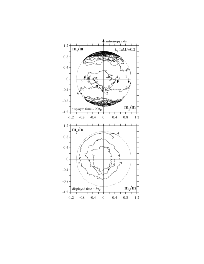
FIGURE 23.: 2D projections of $\vec{m}(t)$, as determined by integration of the stochastic Landau–Lifshitz Eq. (5.20). The anisotropy energy is $-\Delta U(m_{z}/m)^{2}$, no field is applied, and the damping coefficient is $\lambda=0.1$. Upper panel: Projection onto a plane containing the anisotropy axis. Lower panel: Projection onto the plane perpendicular to the anisotropy axis of the first stages of the damped precession down to the $\vec{m}=-m\hat{z}$ potential minimum, after the last barrier crossing.

The projection of $\vec{m}(t)$ onto a plane containing the anisotropy axis $\hat{n}$ (defining the $\hat{z}$ direction in Fig. 23), corresponds to a typical stochastic trajectory that starts close to one of the potential minima ($\vec{m}=m\hat{z}$) and, after some irregular rotations about it, reaches the potential-barrier (equatorial) region, where it wanders for a while, and eventually descends to the other potential minimum. Concerning the projection of this motion onto a plane perpendicular to the anisotropy axis, we have only shown the first stages, after the last potential-barrier crossing, of the damped precession of $\vec{m}$ about the anisotropy field when spiralling down to the bottom of the $m_{z}<0$ potential well.

These graphs reveal the important rôle of the gyromagnetic terms in the stochastic dynamics of the magnetic moment. Thus, the projection of $\vec{m}(t)$ onto the equatorial plane shows some of the typical irregular features of ordinary Brownian motion, although the rotary character is clearly exhibited. Concerning the projection of $\vec{m}(t)$ onto a plane containing the anisotropy axis, it can clearly be seen that crossing the potential barrier does not entail an immediate descent to the other potential minimum, but the gyromagnetic terms together with an appropriate sequence of fluctuating fields can produce a rapid crossing back to the initial potential well.

For an ordinary, non-gyromagnetic system, i.e., a mechanical system with inertia, the inertia guarantees that, unless the system reaches the potential barrier with zero velocity, it will descend to the other potential well with a large probability. Moreover, the forces, after the potential-barrier crossing, accelerate the system downward. In contrast, in the gyromagnetic case the dynamics is “non-inertial” (the equations of motion are of first order in the time). Besides, the anisotropy field $\vec{B}_{{\rm a}}=(B_{K}/m)m_{z}\hat{z}$ indeed drives $\vec{m}$ down to the bottom of the potential well, but this is effected via a damped precession about the anisotropy axis. Moreover, the effective precession “frequency” of this motion $\omega_{{\rm eff}}\propto m_{z}$ is initially rather low because the anisotropy field is low in the potential-barrier region ($m_{z}\simeq 0$). Consequently, in the beginning of the spiraling down after a potential-barrier crossing, the magnetic moment rotates (say, along a parallel of latitude) quite slowly not far from the potential-barrier, so that an appropriate sequence of fluctuations can drive it back to the initial potential well.

What is shown in Fig. 23 is precisely a multiple occurrence of this phenomenon; more than 10 potential-barrier crossings can be identified in the overall excursion between the two potential minima. Besides, the magnetic moment might also have eventually fallen into the original potential well. As will be shown below, none of these processes is infrequent. The physical acumen of Brown (1959) is noteworthy since, on considering the gyromagnetic nature of the dynamics, he posed the possible occurrence of this kind of phenomena in his criticism of the calculation of Néel (1949) of the relaxation time as the inverse of the rate of equatorial crossings of the magnetic moment.

2. The effect of the temperature

In order to assess the effect of the temperature on the dynamics of the magnetic moment, we have displayed in Fig. 25 some typical time evolutions of the projection of $\vec{m}$ onto the anisotropy axis.

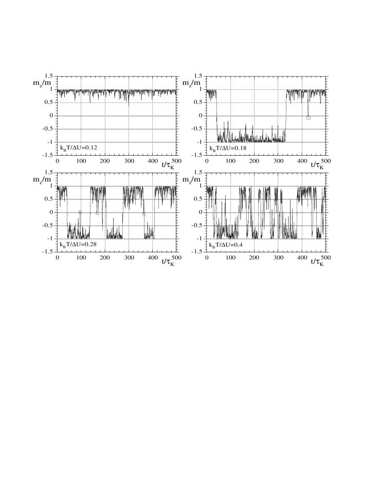
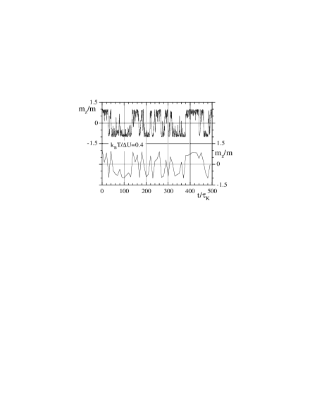
FIGURE 24.: Projection onto the anisotropy axis of $\vec{m}(t)$, as determined by numerical integration of the stochastic Landau–Lifshitz–Gilbert equation (5.20), for various temperatures. The magnetic-anisotropy energy is $-\Delta U(m_{z}/m)^{2}$, $\vec{B}=0$, and $\lambda=0.1$. The small circles mark potential-barrier crossings followed by a back rotation to the initial potential well.

FIGURE 25.: The same as in panel $k_{{\rm B}}T/\Delta U=0.4$ of Fig. 25, but the trajectory has also been plotted with a larger sampling time interval.

As can be seen, at low temperatures (panel $k_{{\rm B}}T/\Delta U=0.12$), the dynamics merely consist of the rotations of the magnetic moment close to the bottom of the potential wells (intra-potential-well relaxation modes), with the over-barrier relaxation mechanism being “blocked.” As the temperature is increased, the magnetic moment can effect over-barrier rotations at the expense of the energy gained from the heat bath, and a number of them do occur during the displayed time interval (panels $k_{{\rm B}}T/\Delta U=0.18$ and $0.28$). Finally, at higher temperatures (panel $k_{{\rm B}}T/\Delta U=0.4$), the magnetic moment effects a considerable number of over-barrier rotations during the observation time interval, exhibiting almost the thermal-equilibrium distribution of orientations.

The curves of Fig. 25 resemble those of the experiments of Wernsdorfer et al. (1997) on individual ferromagnetic nanoparticles (see Fig. 6 in that reference). Furthermore, if the same trajectory is plotted with a larger sampling time interval, in order to mimic the finite resolution time of a measuring device, the resemblance is more apparent, since the curves then have less and wider angles (Fig. 25). (Recall that the strong dependence of the appearance of the time evolution curves on the sampling period is a typical feature of the stochastic dynamics.)

Note finally that in Fig. 25 a number of potential-barrier crossings followed by a rotation back to the original potential well can be identified (marked with small circles): one for $k_{{\rm B}}T/\Delta U=0.18$; three for $k_{{\rm B}}T/\Delta U=0.28$, the one occurring at $\sim 360\,t/\tau_{K}$ being a double crossing-back; and about seven for $k_{{\rm B}}T/\Delta U=0.4$ (not marked for the sake of clarity). It is also to be noted that an apparent single (or double) crossing-back can be multiple instead. Indeed, when the about 10 potential-barrier crossings of Fig. 23 are represented as $m_{z}$ vs. $t$, they seem to be a mere double crossing-back of the potential barrier.

3. Projection of the magnetic moment onto the direction of a probing field

It is also illuminating to show the projection of the trajectories of individual spins onto the direction of a probing field $\Delta\vec{B}(t)=\Delta\vec{B}\cos(\omega t)$. Figure 26 shows this kind of trajectories in the intermediate temperature range.

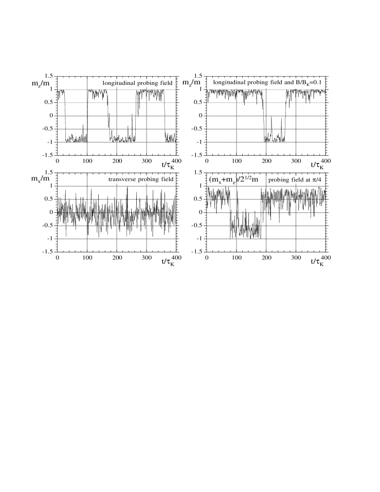
FIGURE 26.: Projection onto the direction of a probing field $\Delta\vec{B}(t)=\Delta\vec{B}\cos(\omega t)$ of $\vec{m}(t)$, as determined by numerical integration of the stochastic Landau–Lifshitz–Gilbert equation (5.20). The magnetic-anisotropy energy is $-\Delta U(m_{z}/m)^{2}$ and all the results are for $k_{{\rm B}}T/\Delta U=0.2$ and $\lambda=0.1$. The displayed time interval corresponds to a complete cycle of the oscillating field ($\omega\tau_{K}/2\pi=0.0025$). In the longitudinal probing field case, results in the presence of a longitudinal bias field are also shown.

The projection onto the anisotropy axis direction ($\Delta\vec{B}\parallel\hat{z}$) exhibits, as in the corresponding case of Fig. 25, a well resolved bistability, and $\vec{m}$ “jumps” from one well to the other a number of times during a cycle of the probing field. Similar features are encountered when a longitudinal bias field is also applied, the main difference being that the lower potential well is less frequented by the magnetic moment. In contrast, the features of the stochastic trajectory obtained by projecting $\vec{m}(t)$ onto a direction perpendicular to the anisotropy axis ($\Delta\vec{B}\perp\hat{z}$) are markedly different (for example, this projection corresponds to plotting the trajectory of the upper panel of Fig. 23 as $m_{x}$ vs. $t$). Here, the response is dominated by the fast ($\sim\tau_{K}$) intra-potential-well relaxation modes, and the transverse projection is a highly irregular sequence of sharp peaks. Finally, the projection of $\vec{m}(t)$ onto $\Delta\vec{B}$ making an intermediate angle with the anisotropy axis ($\pi/4$ for the displayed curve), shows the magnetic bistability of the longitudinal projection, but the fast intra-potential-well motions are superimposed on it. This leads to a less well-resolved magnetic bistability.

Note finally that curves like those of Fig. 26 are the ones “analyzed” by the probing field in a dynamical “measurement.” Recall also that the application of the oscillating field hardly changes the overall features of the curves from the free evolution ones. This is naturally so, since one applies a low enough field in order to probe the intrinsic dynamics of the system.

V.F Dynamical response of the ensemble of spins

Keeping Figs. 25–26 in mind, we shall undertake the study of the dynamical response of an ensemble of classical magnetic moments. As a suitable probe of the intrinsic dynamics of the system, we shall compute the linear dynamical susceptibility, $\chi(\omega)$, as a function of the temperature for various frequencies and orientations of an external probing field $\Delta\vec{B}(t)=\Delta\vec{B}\cos(\omega t)$.

We compute the dynamical response for ensembles of $1000$ magnetic moments. We integrate numerically the stochastic Landau–Lifshitz–Gilbert equation of each spin by means of the stochastic Heun scheme (5.83), and analyze the time evolution of the total magnetic moment of the ensemble; the results for the dynamical susceptibility have typically been averaged over $50$–$100$ cycles of the oscillating field. In addition, in order to reduce the statistical error bars, we apply at each $T$ the largest probing field without leaving the equilibrium linear response range (specifically, we scale the amplitude of the probing field with the temperature according to $m\Delta B=0.3k_{{\rm B}}T$).

The damping coefficient, $\lambda$, the magnetic-anisotropy potential barrier, $\Delta U=Kv$, and the magnitude of the magnetic moment, $m$, are assumed to be the same for each spin. For non-interacting entities the effects of a distribution in these parameters, as typically occurs in nanoparticle ensembles, could be taken into account by an appropriate rescaling and summation of the so-obtained results.

In all the figures which follow, the linear susceptibilities are measured in units of $\mu_{0}m/B_{K}=\mu_{0}m^{2}/2Kv$ [the transverse equilibrium susceptibility per spin at zero temperature in the absence of a bias field; see Eq. (3.82)]. Furthermore, when the statistical error bars of the numerical results are not shown, their size is, at most, that of the plotted symbols. Finally, in order to have a reference of the discussed time scales, we can use the values of Eq. (5.73), so that $\tau_{K}^{-1}\sim 10^{8}$–$10^{10}$ s^-1 and the frequencies employed below ($\omega\tau_{K}/2\pi\sim 10^{-3}$–$10^{-2}$) are then in the MHz range.

1. Dynamical response in the absence of a bias field

We shall first study the response of the spin ensemble in the absence of a constant external field.

a. Longitudinal response.

Figure 27 displays the results for the longitudinal linear dynamical susceptibility vs. the temperature for an ensemble of magnetic moments with parallel anisotropy axes ($\Delta\vec{B}\parallel\hat{z}$).

FIGURE 27.: Longitudinal linear dynamical susceptibility $\chi_{\|}$ vs. $T$ in the absence of a bias field. The symbols are for the numerically computed $\chi_{\|}(\omega,T)$ and the thin solid lines are Eq. (4.2) with $\tau_{\|}$ defined as integral relaxation time [Eq. (5.66)]. The heavy solid line in the upper panel is the thermal-equilibrium susceptibility [Eq. (3.53)]. Inset: Modulus and phase shift $\phi=\arctan(\chi^{\prime\prime}/\chi^{\prime})$ for $\omega\tau_{K}/2\pi=0.0025$.

No bias field has been applied and a damping coefficient $\lambda=0.1$ has been used.

At low temperatures, the longitudinal relaxation time obeys the condition $\tau_{\|}\gg 2\pi/\omega$ [$t_{{\rm m}}(\omega)=2\pi/\omega$ is the dynamical measurement time]. Consequently, during a large number of cycles of the probing field, the probability of over-barrier rotations is almost zero; the response consists of the rotations of the magnetic moments close to the bottom of the potential wells (see the panel $k_{{\rm B}}T/\Delta U=0.12$ of Fig. 25), whose averaged (over the ensemble) projection onto the probing-field direction is quite small (but non zero; see the enlargement of the low-temperature range in Fig. 32). Moreover, as these intra-potential-well relaxation modes are very fast ($\sim\tau_{K}$), this small response is in phase with the probing field [see the low-$T$ part of the phase shift $\phi=\arctan(\chi^{\prime\prime}/\chi^{\prime})$ in the inset of Fig. 27].

As the temperature is increased the magnetic moments can depart from the potential minima by means of the energy gained from the heat bath. Consequently, at a $\omega$-dependent temperature ($k_{{\rm B}}T/Kv\sim 0.1$–$0.2$ for the frequencies employed), it emerges a small probability of surmounting the magnetic-anisotropy potential barrier during a number of cycles of the probing field (this corresponds to the panel $k_{{\rm B}}T/\Delta U=0.18$ of Fig. 25). Accordingly, the averaged response starts to increase steeply with $T$. However, as the thermally activated response mechanism via over-barrier rotations is not efficient enough at these temperatures, the signal exhibits a considerable lag behind the probing field (see the inset of Fig. 27). This is also reflected by the occurrence of a sizable out-of-phase component of the response $\chi_{\|}^{\prime\prime}(T)$ (in fact, the response is mainly “out of phase”).

At higher temperatures, the mechanism of over-barrier rotations becomes increasingly efficient (panel $k_{{\rm B}}T/\Delta U=0.28$ of Fig. 25). Consequently, after exhibiting a maximum, the phase shift starts to decrease, whereas the magnitude of the response still increases steeply with $T$ (see the inset of Fig. 27). However, if the temperature is further increased, the very thermal agitation, which up to these temperatures was responsible for the growth in the magnitude of the response, reaches a level that: (i) efficiently produces over-barrier rotations, allowing the magnetic moments to approximately redistribute according to the instantaneous probing field, but, simultaneously, (ii) disturbs sizably the alignment of the magnetic moments in the probing-field direction. Consequently, at a temperature above that of the phase maximum ($k_{{\rm B}}T/Kv\sim 0.2$–$0.3$ for the frequencies considered), the magnitude of the response has a maximum and starts to decrease with increasing $T$. The frequency-dependent temperature at which this maximum occurs is called the blocking temperature.

Finally, at still higher temperatures ($k_{{\rm B}}T/Kv\geq 0.3$–$0.5$ for the frequencies considered) the inequality $\tau_{\|}\ll 2\pi/\omega$ holds. Thus, in comparison with $\tau_{\|}^{-1}$, the rate of change of the probing field is quasi-stationary. Consequently, the magnetic moments can quickly redistribute according to the conditions set by the instantaneous probing field, almost being in the thermal-equilibrium state associated with it (panel $k_{{\rm B}}T/\Delta U=0.4$ of Fig. 25). Then, the $\chi_{\|}^{\prime}(T)$ curves corresponding to different frequencies sequentially superimpose on the linear equilibrium susceptibility, $\chi_{\|}(T)$, and, correspondingly, $\chi_{\|}^{\prime\prime}(T)$ goes to zero.

The occurrence of a frequency-dependent maximum in the response of a noisy non-linear multi-stable system to a periodic stimulus as a function of the noise intensity, is one of the features usually accompanying stochastic resonance. In this spin-dynamics case, the maximum in the magnitude of the dynamical response as a function of $T$ can be understood in terms of the quoted two-fold rôle played by the temperature: (i) activating the dynamics of over-barrier rotations, enabling the spins to (statistically) follow the instantaneous field, but, (ii) provoking the thermal misalignment of the spins from the driving-field direction. The maximum in the response as a function of $T$ emerges as a result of the competition between these two effects.

b. Transverse response.

We shall now study the transverse dynamical response of an ensemble of magnetic moments with parallel anisotropy axes ($\Delta\vec{B}\perp\hat{z}$). Figure 28 displays the transverse dynamical susceptibility for various frequencies of the probing field (curves labelled 1; results in the presence of a bias field, to be discussed below, are also shown).

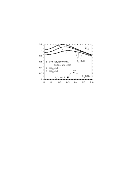
FIGURE 28.: Transverse linear dynamical susceptibility $\chi_{\perp}$ vs. $T$ for the frequencies $\omega\tau_{K}/2\pi=0.001$, $0.0025$, and $0.005$. The damping coefficient is $\lambda=0.1$. Results in the unbiased case ($B=0$) and in the presence of the longitudinal bias fields $B/B_{K}=0.1$ and $0.2$ are shown (for $\omega\tau_{K}/2\pi=0.005$ only). The heavy solid lines are the equilibrium susceptibilities [Eq. (3.70)]. $\chi_{\perp}^{\prime}$ (circles) and $\chi_{\perp}^{\prime\prime}$ (rhombi) have intentionally been plotted with the same scale to show the relative smallness of the latter.

For this transverse probing-field geometry, the mechanism of inter-potential-well rotations plays a secondary dynamical rôle, since it mainly pertains to the components of the magnetic moments perpendicular to the probing field, whereas the response in the probing-field direction is the one analyzed. This consists of intra-potential-well rotations, which are very fast ($\sim\tau_{K}$) in comparison with $t_{{\rm m}}=2\pi/\omega$ (see the panel $m_{x}$ vs. $t$ of Fig. 26). Consequently, the dynamical susceptibilities obtained are close to the equilibrium susceptibility in the whole temperature range. Indeed, the $\chi_{\perp}^{\prime}(T)$ curves corresponding to different frequencies are very close to one another (they visually coincide) and almost describe the equilibrium susceptibility $\chi_{\perp}(T)$ (heavy solid line), while the out-of-phase component $\chi_{\perp}^{\prime\prime}(T)$ is small. Furthermore, $\chi_{\perp}^{\prime\prime}$ is not only small in comparison with $\chi_{\perp}^{\prime}$ but it is also much smaller than the out-of-phase longitudinal susceptibility $\chi_{\|}^{\prime\prime}$ (cf. Fig. 27). Nevertheless, $\chi_{\perp}^{\prime\prime}$ provides an interesting information concerning the dynamics of $\vec{m}$, which will be discussed below.

For the transverse response, the maximum of $\chi_{\perp}^{\prime}$ vs. $T$ is due to the crossover from the free-rotator regime ($\sigma=Kv/k_{{\rm B}}T\ll 1$) to the discrete-orientation regime ($\sigma\gg 1$), induced by the bistable magnetic-anisotropy potential. This is essentially a thermal-equilibrium effect (see Subsec. III.D), with a markedly different character from the dynamical maxima exhibited by the longitudinal susceptibility $\chi_{\|}(\omega,T)$.

c. Response for anisotropy axes distributed at random.

Owing to the linearity of the response, when a distribution in anisotropy axis orientations occurs, $\chi(\omega)$ in the absence of a bias field is merely given by the weighted sum of the longitudinal and transverse dynamical susceptibilities, the weight factors being $\langle\cos^{2}\!\alpha\rangle$ and $\langle\sin^{2}\!\alpha\rangle$, respectively. Here, $\alpha$ is the angle between the anisotropy axis and the probing field, and the angular brackets enclosing functions of $\alpha$ or susceptibilities, stand for average over the anisotropy axis distribution of an ensemble with the same parameters $\lambda$, $\Delta U=Kv$, and $m$.

FIGURE 29.: Linear dynamical susceptibility vs. $T$ for anisotropy axes distributed at random, $B=0$, and $\lambda=0.1$. The symbols are for the numerically computed $\left\langle\chi\right\rangle_{{\rm ran}}$ and the thin solid lines are Eq. (4.2) with $\tau_{\|}$ defined as integral relaxation time [Eq. (5.66)], and $\tau_{\perp}$ given by the effective transverse relaxation time (5.71). The heavy solid line in the upper panel is the thermal-equilibrium susceptibility [Eq. (3.55)]. Inset: Modulus and phase shift $\phi=\arctan(\chi^{\prime\prime}/\chi^{\prime})$ for $\omega\tau_{K}/2\pi=0.0025$.

The linear dynamical susceptibility for anisotropy axes distributed at random ($\langle\cos^{2}\!\alpha\rangle=\langle\sin^{2}\!\alpha\rangle/2=1/3$) is displayed on Fig. 29. The out-of-phase component, $\left\langle\chi^{\prime\prime}\right\rangle_{{\rm ran}}$, is overwhelmingly dominated by the responses to the components of the probing field along the different anisotropy axes, and it is almost $\frac{1}{3}\chi_{\|}^{\prime\prime}(\omega,T)$ (cf. Fig. 27). On the other hand, the in-phase component, $\left\langle\chi^{\prime}\right\rangle_{{\rm ran}}$, is approximately $\frac{1}{3}\chi_{\|}^{\prime}(\omega,T)$ plus a non-uniform upwards shift of magnitude $\frac{2}{3}\chi_{\perp}(T)$, where $\chi_{\perp}(T)$ is the equilibrium transverse susceptibility. This occurs in such a way that: (i) at high temperatures, the Curie law $\left\langle\chi\right\rangle_{{\rm ran}}|_{B=0}=\mu_{0}m^{2}/3k_{{\rm B}}T$ is obeyed (see Subsec. III.D) and, (ii) at temperatures well below the blocking temperatures, the response consists mainly of the projection in the probing field direction of the rotations of the magnetic moments close to the bottom of the potential wells towards the transverse components of the probing field ($\frac{2}{3}\chi_{\perp}|_{T\simeq 0}$). Due to the short characteristic time of these intra-potential-well motions ($\sim\tau_{K}$; see Fig. 26), this low-temperature response is nearly instantaneous and in phase with the probing field (see the inset of Fig. 29).

Note that the large value of the effective $\tau_{0}$ ($\sim 10^{-8}$–$10^{-7}$ s) in the Arrhenius law $\tau_{\|}\simeq\tau_{0}\exp(\Delta U/k_{{\rm B}}T)$, encountered in molecular magnetic clusters having high spin in their ground state, entails that experimental conditions with $\omega/2\pi\sim 10^{3}$–$10^{4}$ Hz already correspond to the frequency range considered here (the MHz range if $\tau_{K}\sim 10^{-10}$–$10^{-8}$ s). Indeed, these systems clearly exhibit the qualitative features of the linear dynamical susceptibility found at “high” (but below ferromagnetic resonance) frequencies: wide maxima in $\chi(\omega,T)$ vs. $T$ for only one potential barrier (relaxation time), sizable $\chi^{\prime}(T)$ at temperatures well below the blocking temperatures, and flattening of the peak of $\chi^{\prime\prime}(T)$ with increasing $\omega$ (Barra et al., 1996; Gomes et al., 1998).

2. Dynamical response in a longitudinal bias field

We shall now study the effects of a constant magnetic field, $\vec{B}$, applied along the common anisotropy axis direction of a spin ensemble with parallel anisotropy axes ($\vec{B}\parallel\hat{z}$).

a. Longitudinal response.

Figure 30 displays the longitudinal ($\Delta\vec{B}\parallel\hat{z}\parallel\vec{B}$) linear dynamical susceptibility of the system for various values of the bias field.

FIGURE 30.: Longitudinal dynamical susceptibility $\chi_{\|}$ vs. $T$, for $\lambda=0.1$, $\omega\tau_{K}/2\pi=0.005$, and various values of the longitudinal bias field. The symbols are for the numerically computed $\chi_{\|}(\omega,T,B)$ and the thin solid lines are Eq. (4.2) with $\tau_{\|}$ defined as integral relaxation time [Eq. (5.66)]. The heavy solid lines in the upper panel are the corresponding equilibrium susceptibilities [Eq. (3.70)]. Inset: Modulus and phase shift $\phi=\arctan(\chi^{\prime\prime}/\chi^{\prime})$ for $B/B_{K}=0.1$.

The qualitative features of the susceptibility curves are similar to those encountered in the unbiased case ($B=0$), and can be interpreted in terms of the same processes:

1. At low temperatures the response consists of the fast rotations of the magnetic moments close to the bottom of the potential wells, with the over-barrier relaxation mechanism being blocked.

2. As $T$ is increased the magnetic moments can depart from the potential minima by means of the energy gained from the heat bath, and the response starts to increase steeply with $T$ (with a sizable lag behind the probing field).

3. If $T$ is further increased the system reaches the regime dominated by inter-potential-well rotations, exhibiting dynamical maxima first in the phase shift and subsequently in the magnitude of the response.

4. In the high-temperature range, the magnetic moments are almost in the thermal-equilibrium state associated with the instantaneous probing field and, hence, $\chi_{\|}^{\prime}(T,B)$ approaches to the linear equilibrium susceptibility while $\chi_{\|}^{\prime\prime}(T,B)$ tends to zero.

Thus, the dynamics is qualitatively similar to the dynamics in the unbiased case, the main difference being that the system now consists of bistable non-symmetrical entities (recall the panel $B/B_{K}=0.1$ of Fig. 26).

We remark in passing that the simple idea that the application of a constant magnetic field reduces the potential barriers, so that the relaxation rate increases and the blocking temperatures shift to lower temperatures, should be viewed with caution. The location of the maximum of the dynamical response do depend on the potential-barrier heights, but also on the form of the equilibrium response, which is markedly different from that of the unbiased case. Indeed, for the frequencies and bias fields considered, the location of the maxima of $\chi_{\|}^{\prime\prime}(T)$ is not very sensitive to the bias field, while the maxima of $\chi_{\|}^{\prime}(T)$ shift slightly to higher temperatures as $B$ increases.

b. Transverse response.

We shall finally consider the transverse dynamical response in the presence of a longitudinal bias field ($\Delta\vec{B}\perp\hat{z}\parallel\vec{B}$). Figure 28 also displays $\chi_{\perp}$ vs. $T$ for various values of the bias field at $\omega\tau_{K}/2\pi=0.005$ (curves labelled 2 and 3). The qualitative features of the response are again similar to those encountered in the unbiased case:

1. The mechanism of inter-potential-well rotations plays a minor dynamical rôle, with the response being dominated by the fast intra-potential-well rotations.

2. The $\chi_{\perp}^{\prime}(T,B)$ curves obtained are rather close to the corresponding equilibrium susceptibilities (heavy solid lines).

3. $\chi_{\perp}^{\prime\prime}(T,B)$ is small in comparison with both $\chi_{\perp}^{\prime}(T,B)$ and $\chi_{\|}^{\prime\prime}(T,B)$.

3. Comparison with different analytical expressions

We shall now compare the linear dynamical susceptibility, obtained by numerical integration of the stochastic Landau–Lifshitz–Gilbert equation, with the heuristic models discussed in Subsec. IV.B and rigorous expressions. In this comparison no adjustable parameter will be employed.

We shall sometimes use the word exact when referring to the numerically computed quantities. Along with the feasible diminishing of the statistical error bars of the computed quantities by averaging over a sufficiently large number of trajectories, we also implicitly mean that the numerical results are exact in the context of the Brown–Kubo–Hashitsume stochastic model.

a. Longitudinal response.

Figure 31 shows the computed $\chi_{\|}(\omega)$ in the unbiased case and in the bias field $B/B_{K}=0.1$.

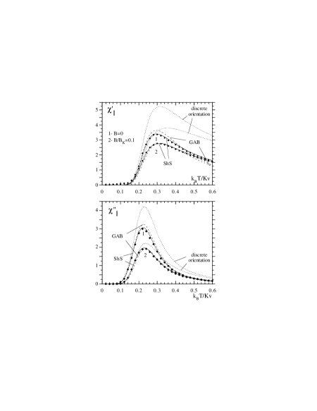
FIGURE 31.: $\chi_{\|}$ vs. $T$ for $B=0$ and $B/B_{K}=0.1$ with $\omega\tau_{K}/2\pi=0.005$ (symbols). The small dashing is for Eq. (4.5), the medium dashing for Eq. (4.2) with the approximate Eq. (3.85), and the solid lines for Eq. (4.2). $\tau_{\|}$ defined as integral relaxation time [Eq. (5.66)] has been incorporated in the three equations.

The results of the heuristic discrete-orientation equation (4.5); Gittleman, Abeles, and Bozowski model [Eq. (4.2) with the approximate Eq. (3.85)]; and Shliomis and Stepanov equation (4.2) are also shown. The longitudinal relaxation time, $\tau_{\|}$, defined as the integral relaxation time $\tau_{\rm int}$, has been used in the three equations.

It is apparent that Eq. (4.5) fails to describe the numerical results; neither is the equilibrium (high-temperature) susceptibility properly described. Actually, the overall failure of this expression could mainly be attributed to the rough approximation used for its equilibrium part [Eq. (3.87)]. The probability that $\vec{m}$ makes a finite angle with the anisotropy axis is completely neglected in such a discrete-orientation equation.

Concerning the Gittleman, Abeles, and Bozowski equation, it is more suitable than the discrete-orientation equation, especially for the matching of $\chi_{\|}^{\prime\prime}(T,B)$, although it fails to describe $\chi_{\|}^{\prime}(T,B)$. Again, not even the equilibrium susceptibility is correctly described; the high-barrier approximation for $\chi_{\|}(T,B)$ occurring in this model [Eq. (3.85)], although better than the discrete-orientation approximation, is still not accurate enough at the relevant temperatures. Furthermore, for bias fields $B/B_{K}\,\raisebox{1.50696pt}{$>$}\raisebox{-2.79857pt}{$\sim$}\,0.15$, the divergence of this model from the exact results becomes dramatic (results not shown).

In contrast, Eq. (4.2) approximates the numerical results reasonably. This is in agreement with the comparison carried out by Raĭkher et al. (1997) of the exact $\chi_{\|}(\omega)$ with what they called the “effective time approximation” [which is indeed equivalent to the use of the longitudinal component of Eq. (4.2) with $\tau_{\|}=\tau_{\rm int}$]. Nevertheless, the exact analytical expression for $\chi_{\|}(\omega)$ comprises an infinite number of Debye-type relaxation mechanisms, namely (see Appendix B)

$$\chi_{\|}(\omega,T,B)=\chi_{\|}(T,B)\sum_{k=1}^{\infty}\frac{a_{k}(T,B)}{1+i\omega/\Lambda_{k}(T,B)}\;,$$ (5.88)

where $a_{k}$ is the amplitude corresponding to the eigenvalue $\Lambda_{k}$ of the Sturm–Liouville equation associated with the Fokker–Planck equation. (Recall that the first non-vanishing eigenvalue, $\Lambda_{1}$, is associated with the inter-potential-well dynamics, whereas the higher-order eigenvalues, $\Lambda_{k}$, $k\geq 2$ are related with the intra-potential-well relaxation modes.) However, the mentioned agreement could be expected in the unbiased case since, as was shown numerically by Coffey et al. (1994): (i) $a_{1}(B=0)\gg a_{k}(B=0),\,\forall k\geq 2$ and (ii) $\Lambda_{1}^{-1}(B=0)\simeq\tau_{\rm int}(B=0)$. Indeed, Coffey, Crothers, Kalmykov and Waldron (1995b) shown that an expression equivalent to the longitudinal component of Eq. (4.2), together with the interpolation formula (5.63) for $\Lambda_{1}^{-1}$, well describes the longitudinal dynamical polarisability of the congeneric nematic liquid crystal with (unbiased) Meier-Saupe potential. (The longitudinal relaxation in this system is mathematically identical with that of classical magnetic moments.) On the other hand, in a constant longitudinal field the higher-order modes can make a substantial contribution in the low-temperature region ($\sigma\gg 1$), and then $\Lambda_{1}^{-1}$ largely deviates from $\tau_{\rm int}$ while $a_{1}\gg a_{k}$ no longer holds (Coffey, Crothers, Kalmykov and Waldron, 1995a; Garanin, 1996). Nevertheless, for the frequencies employed here, the relevant dynamical phenomena occur in the range $\sigma\sim 2$–$10$, so that in the bias fields applied $a_{1}\gg a_{k}$ and $\Lambda_{1}^{-1}\simeq\tau_{\rm int}$ still hold approximately, and hence Eq. (4.2) describes the exact results reasonably.

However, one could expect, even for $B=0$, a significant contribution of the intra-potential-well relaxation modes to the longitudinal response when the over-barrier dynamics is blocked at low $T$ ($\omega/\Lambda_{1}\gg 1$). Indeed, on scrutinizing Figs. 27 and 30, one sees that Eq. (4.2) predicts, both for $B=0$ and $B\neq 0$, a smaller $\chi_{\|}^{\prime}$ when departing from zero at temperatures well below the blocking temperatures than the exact $\chi_{\|}^{\prime}$. In contrast, because the intra-potential-well modes are very fast ($\sim\tau_{K}$), their contribution to the out-of-phase susceptibility is comparatively smaller, so that $\chi_{\|}^{\prime\prime}$ is still described reasonably by the Debye-type term associated with the inter-potential-well dynamics ($\chi_{\|}^{\prime\prime}\simeq\chi_{\|}(\omega/\Lambda_{1})/[1+(\omega/\Lambda_{1})^{2}]$).

These considerations are substantiated by comparing the numerical results with the asymptotic ($\sigma\gg 1$) expression for the longitudinal dynamical susceptibility of the nematic liquid crystal derived by Storonkin (1985), namely

$$\chi_{\|}\simeq\frac{\mu_{0}m^{2}}{k_{{\rm B}}T}\bigg{[}\underbrace{\bigg{(}1-\frac{1}{\sigma}-\frac{3}{4\sigma^{2}}\bigg{)}\frac{1}{1+i\omega/\Lambda_{1}}}_{\mbox{\small inter-potential-well mode}}{}+\underbrace{\frac{1}{8\sigma^{2}}\bigg{(}\frac{1}{1+i\omega/\Lambda_{3}}+\frac{1}{1+i\omega/\Lambda_{5}}\bigg{)}}_{\mbox{\small intra-potential-well modes}}\bigg{]}\;,$$ (5.89)

where [cf. Eq. (5.62) at $B=0$]

$$\Lambda_{1}^{-1} \simeq \tau_{N}\frac{\sqrt{\pi}}{2}\sigma^{-3/2}\exp(\sigma)\Big{(}1+\frac{1}{\sigma}+\frac{7}{4\sigma^{2}}\Big{)}\;,$$ (5.90)

$$\Lambda_{3}^{-1}\simeq\Lambda_{5}^{-1} \simeq \frac{1}{2}\frac{\tau_{{\rm N}}}{\sigma}\Big{(}1+\frac{5}{2\sigma}+\frac{41}{4\sigma^{2}}\Big{)}\;.$$ (5.91)

Note that $(\mu_{0}m^{2}/k_{{\rm B}}T)(1-1/\sigma-3/4\sigma^{2})\simeq\chi_{\|}(T)+{\cal O}(1/\sigma^{2})$ [see Eqs. (3.53) and (b)], while the correction terms in $\Lambda_{1}^{-1}$ agree with those derived by Brown (1979) (see also Coffey et al., 1994). Figure 32 shows that Eq. (5.89) remarkably describes the $B=0$ numerical results at low temperatures.

FIGURE 32.: Detail of the low-temperature part of Fig. 31 showing the effect of the intra-potential-well relaxation modes. The heavy solid line is the equilibrium susceptibility for $B/B_{K}=0.1$, the thin solid lines are for Eq. (4.2), and the dashed-dotted lines for the asymptotic result (5.89) by Storonkin (for $B=0$ only). The out-of-phase components of Eqs. (4.2) and (5.89) visually coincide.

Note that, because $\Lambda_{3,5}\sim\tau_{{\rm N}}/\sigma=\tau_{K}$ [Eq. (5.76)] and $\omega\tau_{K}\ll 1$ for the frequencies considered, it follows that $1/(1+i\omega/\Lambda_{3,5})\simeq 1-i\omega/\Lambda_{3,5}$. Therefore, since $(\mu_{0}m^{2}/k_{{\rm B}}T)\times(1/8\sigma^{2})\propto k_{{\rm B}}T$, Storonkin formula (5.89) yields the low-temperature linear increase of $\chi_{\|}^{\prime}$ with $T$ due to the intra-potential-well relaxation modes, whereas their contribution to $\chi_{\|}^{\prime\prime}$ is smaller by a factor $\omega/\Lambda_{3,5}\sim\omega\tau_{K}$.

Furthermore, the intra-potential-well relaxation modes take a dramatic reflection in the phase shifts (Raĭkher and Stepanov, 1995b). As any expression of the form $\chi(\omega)=\chi/(1+i\omega\tau)$ (Debye-type), the longitudinal component of Eq. (4.2) yields a phase shift

$$\phi_{\|}=\arctan(\omega\tau_{\|})\;,$$ (5.92)

which increases monotonically with decreasing $T$ and, eventually, reaches $\pi/2$ since at low temperatures $\omega\tau_{\|}\gg 1$ (see the insets of Figs. 27 and 30). However, owing to the fact that the fast intra-potential-well relaxation modes yield an almost instantaneous contribution to the response, $\chi_{\|}^{\prime}$ decreases with $T$ less steeply than $\chi_{\|}/[1+(\omega/\Lambda_{1})^{2}]$ at low temperatures, whereas $\chi_{\|}^{\prime\prime}$ is still approximately given by $\chi_{\|}(\omega/\Lambda_{1})/[1+(\omega/\Lambda_{1})^{2}]$. Consequently, the actual phase shift (insets of Figs. 27 and 30), also increases monotonically with decreasing $T$ but, at a temperature close to that of the peak of $\chi_{\|}^{\prime\prime}(T)$, $\phi_{\|}(T)$ exhibits a maximum and then decreases to zero, since at low $T$ the response is again “in phase” with the probing field due to the fast intra-potential-well modes. This behavior of the phase shift is qualitatively similar to that encountered in one-dimensional bistable systems (Morillo and Gómez-Ordóñez, 1993) and ascribed to the crossover from the “high-noise” regime, dominated by inter-potential-well jumps, to the “low-noise” regime, dominated by the fast intra-potential-well motions.

Concerning the phase behavior for non-collinear situations, we must bear in mind that the intra-potential-well motions make a relative contribution to the transverse response much larger than to the longitudinal response. Therefore, as the former contribution is somehow taken into account by Eq. (4.2), via the equilibrium transverse susceptibility, we find that, inasmuch as $\langle\cos^{2}\!\alpha\rangle$ departs from unity, the Shliomis and Stepanov equation describes the low-temperature phase shifts reasonably well (cf. the inset of Fig. 27 with that of Fig. 29). We finally remark that, because the intra-potential-well relaxation modes are very fast and, thus, $\chi_{\|}^{\prime\prime}$ is reasonably described by Eq. (4.2), while $\chi_{\perp}^{\prime\prime}$ is relatively small, the theoretical background of the methods of determination of the energy-barrier distribution of Section IV that are based on the use of the out-of-phase component of the low-frequency equation (4.3), result to be supported in the context of the Brown–Kubo–Hashitsume stochastic model.

b. Transverse response.

Figure 33 displays the corresponding comparison for $\chi_{\perp}(\omega)$ in the unbiased case for various values of the damping coefficient. For the transverse relaxation time, $\tau_{\perp}$, we have employed the effective relaxation time (5.71), which has been derived (Appendix B) from the low-frequency expansion of the equation for $\chi_{\perp}(\omega)$ of Raĭkher and Shliomis (1975; 1994).

FIGURE 33.: Upper panel: $\chi_{\perp}$ vs. $T$ for $B=0$, $\omega\tau_{K}/2\pi=0.005$, and various values of the damping coefficient $\lambda$. The circles are for $\chi_{\perp}^{\prime}$, and the rhombi for $\chi_{\perp}^{\prime\prime}$. The medium dashed line corresponds to the constant $\chi_{\perp}^{\prime}$ given by Eq. (4.4) and the solid lines to Eq. (4.2) with $\tau_{\perp}$ given by the effective transverse relaxation time (5.71). The heavy dashed curve is $\chi_{\perp}^{\prime\prime}$ with $\tau_{\perp}$ given by the $\lambda\gg 1$ result (5.69). Lower panel: Detail of $\chi_{\perp}^{\prime\prime}$ in the intermediate-to-weak damping range together with the exact zero-damping formula (5.93) (dashed-dotted lines).

For the transverse probing-field geometry, the discrete-orientation formula (4.5) predicts obviously an identically zero response, while the Gittleman, Abeles, and Bozowski formula yields a constant $\chi_{\perp}^{\prime}(T)$ and a zero $\chi_{\perp}^{\prime\prime}(T)$. In contrast, the exact $\chi_{\perp}^{\prime}(T)$ is well described by Eq. (4.2), although, because $\omega\tau_{\perp}\ll 1$ holds in the considered frequency range, $\chi_{\perp}^{\prime}(T)$ almost coincides with the equilibrium susceptibility $\chi_{\perp}(T)$. Concerning $\chi_{\perp}^{\prime\prime}(T)$, Eq. (4.2) with the effective expression (5.71) for $\tau_{\perp}$ only matches the out-of-phase response in the low-temperature range for the smallest damping coefficient considered ($\lambda=0.1$). Nevertheless, Fig. 33 shows that, as the damping coefficient is enlarged, the matching between the numerical results and the simple Eq. (4.2) improves if one uses the effective $\tau_{\perp}$ proposed [Eq. (5.71)]. This constitutes an advance over the usual approach, where one employs the $\tau_{\perp}$ derived by the effective-eigenvalue method [Eq. (5.68)], which yields the heavy dashed curve of Fig. 33 irrespective of $\lambda$.

The above comparison is in agreement with that made by Kalmykov and Coffey (1997) of their numerical results, obtained by continued-fraction techniques, with the complete (but approximate) expression for $\chi_{\perp}(\omega)$ of Raĭkher and Shliomis (1975; 1994). The failure of this expression for weak damping was explained in terms of the effects of the gyromagnetic terms of the dynamical equation. When these terms dominate ($\lambda\ll 1$), due to the occurrence of a spread of the precession frequencies of $\vec{m}$ in the anisotropy field at intermediate temperatures (these frequencies are $\propto\gamma B_{K}m_{z}$), the response is not well described by a simple relaxation mechanism. Then, only at low temperatures, where the magnetic moments are concentrated close to the bottom of the potential wells (so the spread in precession frequencies is reduced), the exact results are well described by the $\chi_{\perp}(\omega)$ of Raĭkher and Shliomis.

The effects of the spread of the precession frequencies of $\vec{m}$ in the anisotropy field had already been investigated by Gekht (1983) and independently by Garanin, Ishchenko and Panina (1990). They derived the exact expression for $\chi_{\perp}^{\prime\prime}(\omega,T,B)$ in the $\lambda\to 0$ limit, which accounts for the effects of the phenomenon discussed (the former author employed a Liouville approach while the latter ones started from the Fokker–Planck equation). Their formula can be written as

$$\chi_{\perp}^{\prime\prime}|_{\lambda=0}=\frac{\mu_{0}m^{2}}{k_{{\rm B}}T}\frac{\pi}{2}\frac{\tilde{\omega}}{(2|\sigma|)^{3}}\frac{(2\sigma)^{2}-(\tilde{\omega}-\xi)^{2}}{{\cal Z}}\exp\Big{(}\frac{\tilde{\omega}^{2}-\xi^{2}}{4\sigma}\Big{)}\;,$$ (5.93)

where $\tilde{\omega}=\omega(m/\gamma k_{{\rm B}}T)$, $\xi=mB/k_{{\rm B}}T$, ${\cal Z}$ is the longitudinal partition function (2.25), and $\chi_{\perp}^{\prime\prime}(\omega)$ is non-zero in the interval $(\tilde{\omega}-\xi)^{2}\leq(2\sigma)^{2}$. In order to compare the zero-damping formula (5.93) with the numerical results, we just write $\tilde{\omega}=\omega(2\lambda\tau_{K}\sigma)$, which for fixed $\omega\tau_{K}$ (as occurs in the plots) is a “function” of $\lambda$.

The lower panel of Fig. 33 shows that, for $\lambda=0.5$, the dampingless Eq. (5.93) gives correctly the order of magnitude of the numerical results at intermediate-to-high temperatures, while for $\lambda=0.1$ a good agreement extending down to quite low temperatures can be seen. Since Eq. (5.93) is the exact $\lambda=0$ result, this comparison indicates that, in the intermediate-to-weak damping regime, the contribution of the spread of the precession frequencies of the magnetic moment to $\chi_{\perp}^{\prime\prime}(\omega)$ is sizable in comparison with the effects of the damping. Therefore, by omitting this zero-damping effect one could erroneously extract values of $\lambda$ from the $\chi_{\perp}^{\prime\prime}(\omega)$ data that overestimate the actual $\lambda$ and, for example, infer that the damping in superparamagnets is stronger than it is in fact.

Another important manifestation of this effect was studied by Raĭkher and Stepanov (1995a). The contribution of the damping to the absorption line in intrinsic ferromagnetic resonance provokes a (unbounded) monotonic increase of the linewidth with the temperature, whereas the linewidths experimentally observed in certain magnetic nanoparticle systems are almost independent of the temperature (Hennion et al., 1994). However, the spread of precession frequencies in the anisotropy field also yields a contribution to the linewidths, which in addition saturates at high temperatures. Thus, the combination of both contributions leads to the appearance of an intermediate temperature regime, fairly wide for systems with low damping, in which the linewidth is quasiconstant.

VI Foundation of the stochastic dynamical
equations

VI.A Introduction

In this Section we shall examine various topics related with the foundation of the Brown–Kubo–Hashitsume stochastic model and possible extensions of this model (García-Palacios, 1999).

1. Phenomenological equations

The Brown–Kubo–Hashitsume model is phenomenological inasmuch as is constructed by augmenting known phenomenological equations (Gilbert or Landau–Lifshitz) by fluctuating fields. For subsequent reference, let us first rewrite the basic equations of this model (see Subsec. V.C):

• Stochastic Gilbert equation

  $$\frac{{\rm d}\vec{m}}{{\rm d}t}=\gamma\vec{m}\wedge\bigg{[}\vec{B}_{{\rm eff}}+\vec{b}_{{\rm fl}}(t)-(\gamma m)^{-1}\lambda\frac{{\rm d}\vec{m}}{{\rm d}t}\bigg{]}\;.$$ (6.1)

  This equation is equivalent to the stochastic Landau–Lifshitz–Gilbert equation (5.20), except for a “renormalization” of the gyromagnetic ratio.

• Stochastic Landau–Lifshitz equation

  $$\frac{{\rm d}\vec{m}}{{\rm d}t}=\gamma\vec{m}\wedge\left[\vec{B}_{{\rm eff}}+\vec{b}_{{\rm fl}}(t)\right]-\lambda\frac{\gamma}{m}\vec{m}\wedge\left(\vec{m}\wedge\vec{B}_{{\rm eff}}\right)\;.$$ (6.2)

  This equation may be regarded as the weak damping case ($\lambda\ll 1$) of Eqs. (6.1) or (5.20), although it can be considered as an independent model as well. On the other hand, this is a Langevin equation more archetypal those equations, in the sense that the fluctuating and relaxation (damping) terms are not entangled.

In these dynamical equations $\lambda$ is a dimensionless damping coefficient and $\vec{B}_{{\rm eff}}=-\partial{\cal H}/\partial\vec{m}$ is the (deterministic) effective field associated with the Hamiltonian of the spin ${\cal H}(\vec{m})$. This typically includes Zeeman and magnetic-anisotropy energy terms, e.g., for uniaxial anisotropy with symmetry axis $\vec{n}$

$${\cal H}=-\vec{m}\cdot\vec{B}-{\textstyle\frac{1}{2}}(B_{K}/m)(\vec{m}\cdot\vec{n})^{2}\quad\Longrightarrow\quad\vec{B}_{{\rm eff}}=\vec{B}+\hat{K}\vec{m}\;,$$

where $\hat{K}$ is a second-rank tensor with elements $K_{ij}=(B_{K}/m)n_{i}n_{j}$ [cf. Eq. (5.4)]. On the other hand, $\vec{b}_{{\rm fl}}(t)$ is a fluctuating field, the statistical properties of which are

$$\left\langle b_{{\rm fl},i}(t)\right\rangle=0\;,\qquad\left\langle b_{{\rm fl},i}(t)b_{{\rm fl},j}(t^{\prime})\right\rangle=\frac{2\lambda\delta_{ij}}{\gamma m}\,k_{{\rm B}}T\delta(t-t^{\prime})\;,$$ (6.3)

where we have taken into account that when one starts from the Gilbert equation one must replace $\gamma\to\gamma/(1+\lambda^{2})$ in the results of Section V associated with the stochastic Landau–Lifshitz–Gilbert equation, so that $D_{{\rm LLG}}$ is then identical with $D_{{\rm LL}}$ [see Eq. (5.35)]. Finally, on introducing Eq. (5.33) into Eq. (5.38), the Fokker–Planck equation governing the time evolution of the non-equilibrium probability distribution of spin orientations, associated with the above Langevin equations, can be written as

$$\frac{\partial P}{\partial t}=-\frac{\partial{}}{\partial\vec{m}}\cdot\left\{\gamma\vec{m}\wedge\vec{B}_{{\rm eff}}P-\lambda\frac{\gamma}{m}\vec{m}\wedge\left[\vec{m}\wedge\left(\vec{B}_{{\rm eff}}-k_{{\rm B}}T\frac{\partial{}}{\partial\vec{m}}\right)P\right]\right\}\;,$$ (6.4)

where $(\partial/\partial\vec{m})\cdot\vec{J}=\sum_{i}(\partial J_{i}/\partial m_{i})$ and for the Gilbert case one must replace $\gamma$ by $\gamma/(1+\lambda^{2})$.

The Brown–Kubo–Hashitsume stochastic model has been the basis of significant studies of the dynamics of classical magnetic moments. Nonetheless, there exist important microscopic relaxation mechanisms that cannot be accommodated in the context of this model, inasmuch as they do not produce a field-type perturbation on the spin (“field-type” fluctuations). An important example is the coupling of the spin to the lattice vibrations, which modulate the crystal-field and the exchange and dipole-dipole interactions, and can produce fluctuations of the magnetic-anisotropy potential of the spin (“anisotropy-type” fluctuations).

In order to take this phenomenon into account, Garanin, Ishchenko, and Panina (1990) generalized the above Langevin equations to ${\rm d}\vec{m}/{\rm d}t=\gamma\vec{m}\wedge[\vec{B}_{{\rm eff}}+\vec{b}(t)+\hat{\kappa}(t)\vec{m}]-\vec{R}$. Here, $\vec{R}$ is a relaxation term to be determined and, in analogy with the expression $\vec{B}_{{\rm eff}}=\vec{B}+\hat{K}\vec{m}$ for the effective field, $\vec{b}(t)$ is a stochastic vector that introduces the field-type part of the thermal fluctuations, while $\hat{\kappa}(t)$ is a stochastic second-rank tensor, so that $\hat{\kappa}(t)\vec{m}$ incorporates anisotropy-type fluctuations into the dynamical equation.

On assuming the correlation properties

$$\left\langle b_{i}(t)b_{j}(t^{\prime})\right\rangle = \frac{2\lambda_{ij}}{\gamma m}\,k_{{\rm B}}T\delta(t-t^{\prime})\;,$$

$$\left\langle b_{i}(t)\kappa_{jk}(t^{\prime})\right\rangle = \frac{2\lambda_{i,jk}}{\gamma m}\,k_{{\rm B}}T\delta(t-t^{\prime})\;,$$ (6.5)

$$\left\langle\kappa_{ik}(t)\kappa_{j\ell}(t^{\prime})\right\rangle = \frac{2\lambda_{ik,j\ell}}{\gamma m}\,k_{{\rm B}}T\delta(t-t^{\prime})\;,$$

they constructed the associated Fokker–Planck equation

$$\frac{\partial P}{\partial t}=-\frac{\partial{}}{\partial\vec{m}}\cdot\bigg{\{}\gamma\vec{m}\wedge\vec{B}_{{\rm eff}}P-\bigg{[}\vec{R}-\frac{\gamma}{m}k_{{\rm B}}T\,\vec{m}\wedge\hat{G}\bigg{(}\vec{m}\wedge\frac{\partial{}}{\partial\vec{m}}\bigg{)}\bigg{]}P\bigg{\}}\;,$$ (6.6)

where $\hat{G}$ is a symmetrical second-rank tensor related with the correlation coefficients of the fluctuating terms by

$$G_{ij}=\lambda_{ij}+\sum_{k}(\lambda_{i,jk}+\lambda_{j,ik})m_{k}+\sum_{k\ell}\lambda_{ik,j\ell}m_{k}m_{\ell}\;.$$ (6.7)

The relaxation term $\vec{R}$ was then determined by merely assuming that the Boltzmann distribution $P_{{\rm e}}(\vec{m})\propto\exp[-{\cal H}(\vec{m})/k_{{\rm B}}T]$ is a stationary solution of the Fokker–Planck equation (6.6). This yields $\vec{R}=(\gamma/m)\,\vec{m}\wedge\hat{G}(\vec{m}\wedge\vec{B}_{{\rm eff}})$, so the starting Langevin equation finally reads [cf. Eq. (6.2)]

$$\frac{{\rm d}\vec{m}}{{\rm d}t}=\gamma\vec{m}\wedge\left[\vec{B}_{{\rm eff}}+\vec{b}(t)+\hat{\kappa}(t)\vec{m}\right]-\frac{\gamma}{m}\vec{m}\wedge\hat{G}\left(\vec{m}\wedge\vec{B}_{{\rm eff}}\right)\;.$$ (6.8)

For an arbitrary form of $\hat{G}$ the relaxation term in this equation deviates from the form proposed by Landau and Lifshitz (1935). Only for $G_{ij}=\lambda\delta_{ij}$, which for instance occurs when both the field-type and the anisotropy-type fluctuations are isotropic ($\lambda_{ij}\propto\delta_{ij}$ and $\lambda_{ik,j\ell}\propto\delta_{ij}\delta_{k\ell}$) and there is not interference between them ($\lambda_{i,jk}\equiv 0$), that archetypal relaxation term is recovered and the Fokker–Planck equation of Garanin, Ishchenko, and Panina [Eq. (6.6)] reduces to Eq. (6.4).

2. Dynamical approaches to the phenomenological equations

There have been several attempts to justify, starting from dynamical descriptions of a spin coupled to its surroundings, the phenomenological equations for the stochastic spin dynamics.

Smith and De Rozario (1976) considered a classical magnetic moment $\vec{m}$ coupled to a field $\vec{b}({\bf P},{\bf Q})$ depending on the canonical momenta and coordinates $({\bf P},{\bf Q})$ of the environment. They derived a master equation for $\vec{m}$ by “projecting out” the environment variables, which, when the modulation due to the surroundings is fast in comparison with the precession period of $\vec{m}$, reduces to the Fokker–Planck equation (6.4).

Seshadri and Lindenberg (1982) studied a test spin interacting through a Heisenberg-type Hamiltonian with an environment consisting of other spins. The interaction among the latter was treated by a mean field approach, and a dynamical equation for the test spin was obtained to second order in the spin-environment coupling. The equation derived has the form of a generalized (i.e., containing “memory” terms) Langevin equation, whose fluctuating and relaxation terms naturally obey fluctuation-dissipation relations.

Jayannavar (1991) employed the oscillator-bath representation of the environment (Magalinskiĭ, 1959; Ullersma, 1966; Zwanzig, 1973; Caldeira and Leggett, 1983; Ford, Lewis and O’Connell, 1988), and assumed a coupling linear in both the spin variables and the oscillator coordinates (bilinear coupling). A generalized Langevin equation for the spin was derived, which, in the Markovian approach (no memory) and for isotropic fluctuations, formally reduces to the stochastic Gilbert equation (6.1). (A similar treatment was presented by Klik, 1992.) Equations of Landau–Lifshitz form, akin to those derived by Seshadri and Lindenberg, were also obtained in the weak-coupling regime.

Nevertheless, since spin-environment interactions linear in $\vec{m}$ produce a field-type perturbation on the spin (see below), the treatments mentioned do not account for fluctuations of the magnetic anisotropy of the spin. In this Section, in order to incorporate this phenomenon, we shall extend the bilinear-coupling treatment of Jayannavar by considering general dependences of the spin-environment coupling on the spin variables. Furthermore, we shall also include interactions quadratic in the oscillator variables (the classical analogue of, for example, two-phonon or two-photon relaxation processes), which are essential at sufficiently high temperatures. Because the ordinary formalism of the environment of independent oscillators is not directly applicable when such quadratic couplings are included, we shall resort to a perturbational expansion in the spin-environment coupling, which is inspired on that of Cortés, West and Lindenberg (1985).

We shall obtain dynamical equations for the spin that have the structure of generalized Langevin equations with fluctuating terms $\gamma\vec{m}\wedge\vec{b}_{{\rm fl}}(\vec{m},t)$ and concomitant relaxation terms. These will have the form of a vector product of $\vec{m}(t)$ with a memory integral, which includes $({\rm d}\vec{m}/{\rm d}t)(t^{\prime})$ or $(\vec{m}\wedge\vec{B}_{{\rm eff}})(t^{\prime})$ for weak coupling, taken along the past history of the spin ($t^{\prime}\leq t$). In the Markovian approach, the equations derived will reduce to the form

$$\frac{{\rm d}\vec{m}}{{\rm d}t}=\gamma\vec{m}\wedge[\vec{B}_{{\rm eff}}+\vec{b}_{{\rm fl}}(\vec{m},t)]-\vec{R}\;,$$

where for couplings linear in the environmental coordinates the relaxation term reads $\vec{R}=(1/m)\,\vec{m}\wedge\hat{\Lambda}^{\scriptscriptstyle{\rm(L)}}({\rm d}\vec{m}/{\rm d}t)$ or $\vec{R}=(\gamma/m)\,\vec{m}\wedge\hat{\Lambda}^{\scriptscriptstyle{\rm(L)}}(\vec{m}\wedge\vec{B}_{{\rm eff}})$ for weak coupling, $\hat{\Lambda}^{\scriptscriptstyle{\rm(L)}}$ being a second-rank tensor depending on the structure of the coupling. In addition, when interactions quadratic in the environment variables are also taken into account, the relaxation term will depend explicitly on the temperature and, in the Markovian approach, $\vec{R}$ will take the form $\vec{R}=(\gamma/m)\,\vec{m}\wedge\hat{\Lambda}(\vec{m}\wedge\vec{B}_{{\rm eff}})$, with $\hat{\Lambda}=\hat{\Lambda}^{\scriptscriptstyle{\rm(L)}}+k_{{\rm B}}T\,\hat{\Lambda}^{\scriptscriptstyle{\rm(Q)}}$, where the additional tensor $\hat{\Lambda}^{\scriptscriptstyle{\rm(Q)}}$ is determined by the quadratic portion of the coupling.

Since the fluctuating effective field $\vec{b}_{{\rm fl}}(\vec{m},t)$ will depend in general on $\vec{m}$, it can incorporate fluctuations of the magnetic anisotropy of the spin. For instance, when the spin-environment interaction includes terms up to quadratic in the spin variables, $\vec{b}_{{\rm fl}}(\vec{m},t)$ can be written as $\vec{b}(t)+\hat{\kappa}(t)\vec{m}$, with the correlation coefficients of the fluctuating terms being related with the tensors $\hat{\Lambda}$ by expressions identical with Eq. (6.7). In this way, the generalization of the classic Brown–Kubo–Hashitsume model effected by Garanin, Ishchenko, and Panina will formally be obtained.

VI.B Free dynamics and canonical variables

The dynamical equation for an isolated classical spin with Hamiltonian ${\cal H}(\vec{m})$ is

$$\frac{{\rm d}\vec{m}}{{\rm d}t}=\gamma\vec{m}\wedge\vec{B}_{{\rm eff}}\;,\qquad\vec{B}_{{\rm eff}}=-\frac{\partial{\cal H}}{\partial\vec{m}}\;.$$ (6.9)

By means of the formula (5.40) for the gradient operator in spherical coordinates, these vectorial equations, which merely express the precession of $\vec{m}$ about the instantaneous effective field, can be written as

$$\frac{{\rm d}\varphi}{{\rm d}t}=-\frac{\gamma}{m}\frac{1}{\sin\vartheta}\frac{\partial{\cal H}}{\partial\vartheta}\;,\qquad\frac{{\rm d}\vartheta}{{\rm d}t}=\frac{\gamma}{m}\frac{1}{\sin\vartheta}\frac{\partial{\cal H}}{\partial\varphi}\;,$$ (6.10)

where $\varphi$ and $\vartheta$ are, respectively, the azimuthal and polar angles of $\vec{m}$. Furthermore, these formulae are equivalent to the Hamilton equations

$$\frac{{\rm d}q}{{\rm d}t}=\frac{\partial{\cal H}}{\partial p}\;,\qquad\frac{{\rm d}p}{{\rm d}t}=-\frac{\partial{\cal H}}{\partial q}\;,$$

with the conjugate canonical variables

$$q=\varphi\;,\qquad p=m_{z}/\gamma\;.$$ (6.11)

In terms of the variables (6.11) the Cartesian components of the magnetic moment are given by

$$m_{x}=\sqrt{m^{2}-(\gamma p)^{2}}\cos q\;,\quad m_{y}=\sqrt{m^{2}-(\gamma p)^{2}}\sin q\;,\quad m_{z}=\gamma p\;.$$

From these expressions for $m_{i}(p,q)$ and the definition of the Poisson bracket of two arbitrary dynamical variables

$$\big{\{}A,B\big{\}}\equiv\frac{\partial A}{\partial q}\frac{\partial B}{\partial p}-\frac{\partial A}{\partial p}\frac{\partial B}{\partial q}\;,$$

one can readily obtain the customary Poisson-bracket (“commutation”) relations among the spin variables

$$\big{\{}m_{i},m_{j}\big{\}}=\gamma\sum_{k}\epsilon_{ijk}m_{k}\;,$$

where $\epsilon_{ijk}$ is the Levi–Civita symbol. In addition, on using the chain rule of the Poisson bracket, namely

$$\big{\{}f,g\big{\}}=\sum_{i,k}\frac{\partial f}{\partial x_{i}}\frac{\partial g}{\partial x_{k}}\big{\{}x_{i},x_{k}\big{\}}\;,\qquad x_{i}=x_{i}(p,q)\;,$$

one gets the useful relation (cf. Eq. (13) by Smith and De Rozario, 1976)

$$\big{\{}m_{i},V(\vec{m})\big{\}}=-\gamma\bigg{(}\vec{m}\wedge\frac{\partial V}{\partial\vec{m}}\bigg{)}_{i}\;,$$ (6.12)

which is valid for any function of the spin variables $V(\vec{m})$.

Note finally that one can conversely postulate the relations $\{m_{i},m_{j}\}=\gamma\sum_{k}\epsilon_{ijk}m_{k}$ and then derive Eq. (6.9) starting from the basic Hamiltonian evolution equation ${\rm d}m_{i}/{\rm d}t=\{m_{i},{\cal H}\}$ and using Eq. (6.12). This can be considered as a justification of the presence of the expression $\vec{B}_{{\rm eff}}=-\partial{\cal H}/\partial\vec{m}$ in the dynamical equations for a classical spin.

VI.C Dynamical equations for couplings linear in the environment variables

We shall now study a classical spin surrounded by an environment that can be represented by a set of independent classical harmonic oscillators. In spite of its academic appearance, those oscillators can correspond to the normal modes of an electromagnetic field, the lattice vibrations (in the harmonic approximation), or they can be an effective low-energy description of a more general surrounding medium (Caldeira and Leggett, 1983). We shall assume that the spin-environment interaction is linear in the coordinates of the oscillators but otherwise arbitrary in the spin variables. In this way, fluctuations of the magnetic anisotropy of the spin will be incorporated in the dynamical equations.

1. The spin-environment Hamiltonian

The total system consisting of the spin (the “system of interest”) plus the oscillators representing the environment forms a closed dynamical system that we shall describe by augmenting the isolated-spin Hamiltonian as follows

$${\cal H}_{\rm T}={\cal H}(\vec{m})+\sum_{\alpha}{\textstyle\frac{1}{2}}\Big{\{}P_{\alpha}^{2}+\omega_{\alpha}^{2}\Big{[}Q_{\alpha}+\frac{\varepsilon}{\omega_{\alpha}^{2}}F_{\alpha}(\vec{m})\Big{]}^{2}\Big{\}}\;.$$ (6.13)

Here, $\alpha$ is an oscillator index [e.g., the pair $(\vec{k},s)$ formed by the wave-vector and branch index of a normal mode of the environment], and the coupling terms $F_{\alpha}(\vec{m})$ are arbitrary functions of the spin variables (typically polynomials in $\vec{m}$). These terms may depend on the parameters of the oscillators $\omega_{\alpha},$ but not on their dynamical variables $P_{\alpha},Q_{\alpha}$. On the other hand, for the sake of convenience in keeping track of the various orders, we have introduced a spin-environment coupling constant $\varepsilon$, which in the weak-coupling approximation will be considered small.

The terms proportional to $F_{\alpha}^{2}$, which emerge when squaring $Q_{\alpha}+(\varepsilon/\omega_{\alpha}^{2})F_{\alpha}$, are “counter-terms” introduced to balance the coupling-induced renormalization of the Hamiltonian of the spin. The formalism takes as previously considered whether such a renormalization actually occurs for a given interaction (Caldeira and Leggett, 1983), so that ${\cal H}$ would already include it (whenever exists). An advantage of this convention is that one deals with the experimentally accessible energy of the spin, instead of the “bare” one, which might be difficult to determine.

The introduction of non-linear coupling terms $F_{\alpha}(\vec{m})$, as otherwise occur in various relevant situations ($F_{\alpha}\propto\sum m_{k}m_{\ell}$ for the magneto-elastic coupling of $\vec{m}$ to the lattice vibrations), will be essential to get fluctuations of the magnetic anisotropy of the spin. The starting Hamiltonian in the work of Jayannavar (1991) was similar to (6.13) with a special type of linear $F_{\alpha}(\vec{m})$: the component $m_{i}$ of the magnetic moment was coupled to the $i$th Cartesian component $Q_{\alpha,i}$ of certain three-dimensional oscillators. This specific bilinear interaction yielded, not only field-type fluctuations, but also uncorrelated ones. [Klik (1992) also considered couplings non-linear in $\vec{m}$, but in that work the focus was on the existence of thermal equilibrium in the Markovian limit.]

2. Dynamical equations: general case

For the sake of simplicity in notation but also of generality, we cast the Hamiltonian (6.13) into the form

$${\cal H}_{\rm T}={\cal H}^{({\rm m})}(p,q)+\sum_{\alpha}{\textstyle\frac{1}{2}}\left(P_{\alpha}^{2}+\omega_{\alpha}^{2}Q_{\alpha}^{2}\right)+\varepsilon\sum_{\alpha}Q_{\alpha}F_{\alpha}(p,q)\;,$$ (6.14)

where $q$ and $p$ are the canonical coordinate and conjugate momentum of a system with Hamiltonian ${\cal H}(p,q)$ [in the spin-dynamics case $p$ and $q$ are given by Eqs. (6.11)], and the “modified” system Hamiltonian ${\cal H}^{({\rm m})}$ augments ${\cal H}$ by the aforementioned counter-terms

$${\cal H}^{({\rm m})}={\cal H}+\frac{\varepsilon^{2}}{2}\sum_{\alpha}\frac{F_{\alpha}^{2}}{\omega_{\alpha}^{2}}\;.$$ (6.15)

The equation of motion for any dynamical variable $C$ without explicit dependence on the time, $\partial C/\partial t\equiv 0$, is given by the basic Hamiltonian evolution equation

$$\frac{{\rm d}C}{{\rm d}t}=\big{\{}C,{\cal H}_{\rm T}\big{\}}\;,$$

where the whole Poisson bracket is given by

$$\big{\{}A,B\big{\}}\equiv\frac{\partial A}{\partial q}\frac{\partial B}{\partial p}-\frac{\partial A}{\partial p}\frac{\partial B}{\partial q}+\sum_{\alpha}\frac{\partial A}{\partial Q_{\alpha}}\frac{\partial B}{\partial P_{\alpha}}-\frac{\partial A}{\partial P_{\alpha}}\frac{\partial B}{\partial Q_{\alpha}}\;.$$

Therefore, the (coupled) equations of motion for any dynamical variable (observable) of the system $A(p,q)$ and the environment variables read ($C=A,P_{\alpha}$, and $Q_{\alpha}$)

$$\frac{{\rm d}A}{{\rm d}t} = \big{\{}A,{\cal H}^{({\rm m})}\big{\}}+\varepsilon\sum_{\alpha}Q_{\alpha}\big{\{}A,F_{\alpha}\big{\}}\;,$$ (6.16)

$$\frac{{\rm d}Q_{\alpha}}{{\rm d}t} = P_{\alpha}\;,\qquad\frac{{\rm d}P_{\alpha}}{{\rm d}t}=-\omega_{\alpha}^{2}Q_{\alpha}-\varepsilon F_{\alpha}\;.$$ (6.17)

The goal is to derive a dynamical equation for $A(p,q)$ involving the system variables only (reduced dynamical equation). Then, the corresponding equation for the spin will be obtained by replacing $A(p,q)$ in that equation by the Cartesian components of $\vec{m}$ [Eq. (VI.B)].

On considering that in Eqs. (6.17) the term $-\varepsilon F_{\alpha}(t)=-\varepsilon F_{\alpha}[p(t),q(t)]$ plays the rôle of a time-dependent forcing on the oscillators, those equations can be explicitly integrated, yielding

$$Q_{\alpha}(t)=Q_{\alpha}^{{\rm h}}(t)-\frac{\varepsilon}{\omega_{\alpha}}\int_{t_{0}}^{t}\!\!{\rm d}{t^{\prime}}\,\sin[\omega_{\alpha}(t-t^{\prime})]F_{\alpha}(t^{\prime})\;,$$ (6.18)

where

$$Q_{\alpha}^{{\rm h}}(t)=Q_{\alpha}(t_{0})\cos[\omega_{\alpha}(t-t_{0})]+[P_{\alpha}(t_{0})/\omega_{\alpha}]\sin[\omega_{\alpha}(t-t_{0})]\;,$$ (6.19)

are the solutions of the homogeneous system of equations for the oscillators in the absence of the system-environment interaction (proper modes of the environment). Then, on integrating by parts in Eq. (6.18) one gets for the combination $\varepsilon Q_{\alpha}$ that appears in Eq. (6.16)

$$\varepsilon Q_{\alpha}(t)=f_{\alpha}(t)-\left[{\cal K}_{\alpha}(t-t^{\prime})F_{\alpha}(t^{\prime})\right]_{t^{\prime}=t_{0}}^{t^{\prime}=t}+\int_{t_{0}}^{t}\!\!{\rm d}{t^{\prime}}\,{\cal K}_{\alpha}(t-t^{\prime})\frac{{\rm d}F_{\alpha}}{{\rm d}t}(t^{\prime})\;,$$ (6.20)

where

$$f_{\alpha}(t)=\varepsilon Q_{\alpha}^{{\rm h}}(t)\;,\qquad{\cal K}_{\alpha}(\tau)=\frac{\varepsilon^{2}}{\omega_{\alpha}^{2}}\cos(\omega_{\alpha}\tau)\;.$$ (6.21)

Next, in order to eliminate the environment variables from the equation for $A(p,q)$, one substitutes Eq. (6.20) back into Eq. (6.16). This yields a term $\sum_{\alpha}\big{\{}A,F_{\alpha}\big{\}}{\cal K}_{\alpha}(t-t_{0})F_{\alpha}(t_{0})$ that depends on the initial state of the system $(p(t_{0}),q(t_{0}))$ and produces a transient response that can be ignored in the long-time dynamics (we shall however return to this question below). The parallel term $-\sum_{\alpha}\big{\{}A,F_{\alpha}\big{\}}{\cal K}_{\alpha}(0)F_{\alpha}(t)$, which is derivable from a Hamiltonian, is exactly balanced by the term emerging from the counter-terms in $\big{\{}A,{\cal H}^{({\rm m})}\big{\}}$. This can be shown by using $-\sum_{\alpha}\big{\{}A,F_{\alpha}\big{\}}{\cal K}_{\alpha}(0)F_{\alpha}=\big{\{}A,-{\textstyle\frac{1}{2}}\sum_{\alpha}{\cal K}_{\alpha}(0)F_{\alpha}^{2}\big{\}}$, which follows from the product rule of the Poisson bracket

$$\big{\{}A,BC\big{\}}=\big{\{}A,B\big{\}}C+\big{\{}A,C\big{\}}B\;,$$ (6.22)

and then using ${\cal K}_{\alpha}(0)=\varepsilon^{2}/\omega_{\alpha}^{2}$ [see Eq. (6.21)].

Therefore, one is finally left with the reduced dynamical equation

$$\frac{{\rm d}A}{{\rm d}t}=\big{\{}A,{\cal H}\big{\}}+\sum_{\alpha}\big{\{}A,F_{\alpha}\big{\}}\bigg{[}f_{\alpha}(t)+\int_{t_{0}}^{t}\!\!{\rm d}{t^{\prime}}\,{\cal K}_{\alpha}(t-t^{\prime})\frac{{\rm d}F_{\alpha}}{{\rm d}t}(t^{\prime})\bigg{]}\;,$$ (6.23)

where the first term yields the free (conservative) time evolution of the system, whereas the second term incorporates the effects of the interaction of the system with its environment. The terms $f_{\alpha}(t)$ are customarily interpreted as fluctuating “forces” (or “fields”), while the integral term, which keeps in general memory of the previous history of the system, provides the relaxation due to the interaction with the surrounding medium. [Note that without the integration by parts yielding Eq. (6.20), the Hamiltonian (renormalization) terms would occur inconveniently mixed in the integral term.]

The origin of both types of terms can be traced back as follows. Recall that in Eq. (6.18) the time evolution of the oscillators has formally been written as if they were driven by (time-dependent) forces $-\varepsilon F_{\alpha}[p(t^{\prime}),q(t^{\prime})]$ depending on the state of the system. Therefore, $Q_{\alpha}(t)$ consists of the sum of the proper (free) mode $Q_{\alpha}^{{\rm h}}(t)$ and the driven-type term, which naturally depends on the “forcing” (state of the system) at previous times. Then, the replacement of $Q_{\alpha}$ in the equation for the system variables by the driven-oscillator solution incorporates:

1. The time-dependent modulation due to the proper modes of the environment.

2. The “back-reaction” on the system of its preceding action on the surrounding medium.

Thus, the formalism leads to a description in terms of a reduced number of dynamical variables at the expense of both explicitly time-dependent (fluctuating) terms and history-dependent (relaxation) terms (see Table VI).

TABLE VI.: Terms incorporating the effects of the interaction of the system with the surrounding medium in the reduced dynamical equation (6.23).

term	mechanism	interpretation
$f_{\alpha}(t)$	time-dependent modulation due to the proper modes of the environment	fluctuating term
integral term	back-reaction on the system of its preceding action on the environment	relaxation term

Archetypal example: the Brownian particle.

In order to particularize these general expressions to definite situations, the structure of the coupling terms $F_{\alpha}$ needs to be specified. For instance, on setting $F_{\alpha}(p,q)=-{\scriptstyle C}_{\alpha}q$ (bilinear coupling), where the ${\scriptstyle C}_{\alpha}={\scriptstyle C}_{\alpha}(\omega_{\alpha})$ are coupling constants, and writing down Eq. (6.23) for $A=q$ and $A=p$ with help from $\big{\{}p,B\big{\}}=-\partial B/\partial q$ and $\big{\{}q,B\big{\}}=\partial B/\partial p$, one gets the celebrated generalized Langevin equation for a “Brownian” particle (Zwanzig, 1973)

$$\frac{{\rm d}q}{{\rm d}t}=\frac{\partial{\cal H}}{\partial p}\;,\qquad\frac{{\rm d}p}{{\rm d}t}=-\frac{\partial{\cal H}}{\partial q}+f(t)-\int_{t_{0}}^{t}\!\!{\rm d}{t^{\prime}}\,{\cal K}(t-t^{\prime})\frac{{\rm d}q}{{\rm d}t}(t^{\prime})\;.$$ (6.24)

Here, $f(t)=\sum_{\alpha}{\scriptstyle C}_{\alpha}f_{\alpha}(t)$ is the fluctuating force and ${\cal K}(\tau)=\sum_{\alpha}{\scriptstyle C}_{\alpha}^{2}{\cal K}_{\alpha}(\tau)$ is the memory kernel, the relaxation term associated with which comprises minus the velocity $-({\rm d}q/{\rm d}t)(t^{\prime})$ of the particle (viscous damping).

In general, when $\big{\{}A,F_{\alpha}\big{\}}$ in Eq. (6.23) is not constant, the fluctuating terms $f_{\alpha}(t)$ enter multiplying the system variables (multiplicative fluctuations). In this example, owing to the fact that $\big{\{}q,-{\scriptstyle C}_{\alpha}q\big{\}}=0$ and $\big{\{}p,-{\scriptstyle C}_{\alpha}q\big{\}}={\scriptstyle C}_{\alpha}$, the fluctuations are additive.

3. Dynamical equations: the spin-dynamics case

Let us now particularize the above results to the dynamics of a classical spin. Here, we introduce the coupling functions

$$F_{\alpha}(\vec{m})=\sum_{{\bf l}}{\scriptstyle C}_{\alpha}^{{\bf l}}V_{{\bf l}}(\vec{m})\;,$$ (6.25)

where ${\bf l}$ stands for a general index depending on the type of interaction, the coefficients ${\scriptstyle C}_{\alpha}^{{\bf l}}$ are spin-environment coupling constants, and the terms $V_{{\bf l}}(\vec{m})$ are certain functions of the spin variables. In order to motivate this expression, consider, for example, the magneto-elastic coupling of $\vec{m}$ to the lattice vibrations. The index ${\bf l}$ then stands for a pair of Cartesian indices $(ij)$ and $V_{{\bf l}}\to V_{ij}=\sum_{k\ell}a_{ij,k\ell}m_{k}m_{\ell}$, where the $a_{ij,k\ell}$ are magneto-elastic coefficients.

In order to derive the reduced dynamical equation for the spin, we merely put $A=m_{i}$, $i=x,y,z$, in Eq. (6.23), and then use Eq. (6.12) to calculate the Poisson brackets required. On gathering the results so-obtained in vectorial form and using $\vec{B}_{{\rm eff}}=-\partial{\cal H}/\partial\vec{m}$ and ${\rm d}V_{{\bf l^{\prime}}}/{\rm d}t=(\partial V_{{\bf l^{\prime}}}/\partial\vec{m})\cdot({\rm d}\vec{m}/{\rm d}t)$, we arrive at

$$\frac{{\rm d}\vec{m}}{{\rm d}t}=\gamma\vec{m}\wedge\bigg{\{}\vec{B}_{{\rm eff}}+\vec{b}_{{\rm fl}}(\vec{m},t)-\int_{t_{0}}^{t}\!\!{\rm d}{t^{\prime}}\,\hat{\Gamma}^{\scriptscriptstyle{\rm(L)}}(\vec{m};t,t^{\prime})\frac{{\rm d}\vec{m}}{{\rm d}t}(t^{\prime})\bigg{\}}\;.$$ (6.26)

In this equation the fluctuating magnetic field is given by

$$\vec{b}_{{\rm fl}}(\vec{m},t)=-\sum_{{\bf l}}f_{{\bf l}}(t)\frac{\partial V_{{\bf l}}}{\partial\vec{m}}\;,$$ (6.27)

which involves the environmental proper modes via the fluctuating sources

$$f_{{\bf l}}(t)=\varepsilon\sum_{\alpha}{\scriptstyle C}_{\alpha}^{{\bf l}}Q_{\alpha}^{{\rm h}}(t)\;.$$ (6.28)

On the other hand, the relaxation tensor in Eq. (6.26) reads

$$\hat{\Gamma}^{\scriptscriptstyle{\rm(L)}}(\vec{m};t,t^{\prime})=\sum_{{\bf l},{\bf l^{\prime}}}{\cal K}_{{\bf l}{\bf l^{\prime}}}(t-t^{\prime})\frac{\partial V_{{\bf l}}}{\partial\vec{m}}(t)\frac{\partial V_{{\bf l^{\prime}}}}{\partial\vec{m}}(t^{\prime})\;,$$ (6.29)

where the memory kernel is given by

$${\cal K}_{{\bf l}{\bf l^{\prime}}}(\tau)=\varepsilon^{2}\sum_{\alpha}\frac{{\scriptstyle C}_{\alpha}^{{\bf l}}{\scriptstyle C}_{\alpha}^{{\bf l^{\prime}}}}{\omega_{\alpha}^{2}}\cos(\omega_{\alpha}\tau)\;.$$ (6.30)

Equation (6.26) contains ${\rm d}\vec{m}/{\rm d}t$ on its right-hand side, so it will be referred to as a Gilbert-type equation [cf. Eq. (6.1)]. For $\varepsilon\ll 1$, on replacing perturbatively that derivative by its conservative part, ${\rm d}\vec{m}/{\rm d}t\simeq\gamma\vec{m}\wedge\vec{B}_{{\rm eff}}$, one gets the weak-coupling Landau–Lifshitz-type equation

$$\frac{{\rm d}\vec{m}}{{\rm d}t}=\gamma\vec{m}\wedge\left[\vec{B}_{{\rm eff}}+\vec{b}_{{\rm fl}}(\vec{m},t)\right]-\gamma\vec{m}\wedge\bigg{\{}\int_{t_{0}}^{t}\!\!{\rm d}{t^{\prime}}\,\gamma\hat{\Gamma}^{\scriptscriptstyle{\rm(L)}}(\vec{m};t,t^{\prime})\left(\vec{m}\wedge\vec{B}_{{\rm eff}}\right)(t^{\prime})\bigg{\}}\;,$$ (6.31)

which describes weakly damped precession.

For spin-environment interactions linear in the environment variables but being otherwise arbitrary functions of $\vec{m}$, Eqs. (6.26) and (6.31) are the desired reduced dynamical equations for the spin. They have the structure of generalized Langevin equations with fluctuating terms $\gamma\vec{m}\wedge\vec{b}_{{\rm fl}}(\vec{m},t)$ (associated with the modulation by the proper modes of the environment) and history-dependent relaxation terms (corresponding to the back-reaction on the spin of its previous action on the surrounding medium).

Note that $f_{{\bf l}}(t)$ [Eq. (6.28)] is a sum of a large number of sinusoidal terms with different frequencies and phases; this can give to $f_{{\bf l}}(t)$ the form of a highly irregular function of $t$ that is expected for a fluctuating term. However, for a general form of the coupling functions $V_{{\bf l}}(\vec{m})$, the term $\vec{b}_{{\rm fl}}(\vec{m},t)$ cannot be interpreted as a fluctuating ordinary field, since it may depend on $\vec{m}$, but it is rather a fluctuating effective field to be added to the deterministic effective field $\vec{B}_{{\rm eff}}=-\partial{\cal H}/\partial\vec{m}$ [Eq. (6.9)]. This can be illustrated by phrasing the discussion in terms of the fluctuating part of the energy of the spin, namely [see Hamiltonian (6.14)]: ${\cal H}_{{\rm fl}}=\varepsilon\sum_{\alpha}Q_{\alpha}^{{\rm h}}(t)F_{\alpha}(\vec{m})$. From this definition one first gets

$${\cal H}_{{\rm fl}}(\vec{m},t)=\sum_{{\bf l}}f_{{\bf l}}(t)V_{{\bf l}}(\vec{m})\;,\qquad\vec{b}_{{\rm fl}}(\vec{m},t)=-\frac{\partial{\cal H}_{{\rm fl}}}{\partial\vec{m}}\;,$$ (6.32)

so that $\vec{b}_{{\rm fl}}$ can be derived from ${\cal H}_{{\rm fl}}$ in the same way as $\vec{B}_{{\rm eff}}$ is obtained from ${\cal H}$. Next, recall that the non-linear part of ${\cal H}(\vec{m})$ carries the anisotropy-energy terms, e.g., ${\cal H}=-\vec{m}\cdot\vec{B}-{\textstyle\frac{1}{2}}(B_{K}/m)(\vec{m}\cdot\vec{n})^{2}$ in a uniaxial crystal. Analogously, ${\cal H}_{{\rm fl}}$ has the form ${\cal H}_{{\rm fl}}(\vec{m},t)=-\vec{m}\cdot\vec{b}_{{\rm fl}}(t)$, with $\vec{b}_{{\rm fl}}$ independent of $\vec{m}$, only for linear $V_{{\bf l}}(\vec{m})$ (bilinear coupling), so that the non-linear part of $V_{{\bf l}}(\vec{m})$ incorporates fluctuations of the magnetic anisotropy of the spin.

To illustrate, if the spin-environment interaction includes up to quadratic terms in $\vec{m}$, one can write the coupling functions $V_{{\bf l}}(\vec{m})$ as

$$V_{{\bf l}}(\vec{m})=\sum_{i}v_{{\bf l},i}m_{i}+{\textstyle\frac{1}{2}}\sum_{ij}w_{{\bf l},ij}m_{i}m_{j}\;,$$ (6.33)

where the constants $v_{{\bf l},i}$ and $w_{{\bf l},ij}$ incorporate the symmetry of the interaction. In this case, the fluctuating effective field (6.27) can be cast into the form [cf. Eq. (6.8)]

$$\vec{b}_{{\rm fl}}(\vec{m},t)=\vec{b}(t)+\hat{\kappa}(t)\vec{m}\;,$$ (6.34)

with the following expressions for the fluctuating sources $\vec{b}(t)$ and $\hat{\kappa}(t)$ in terms of the coupling constants

$$b_{i}(t)=-\sum_{{\bf l}}f_{{\bf l}}(t)v_{{\bf l},i}\;,\qquad\kappa_{ij}(t)=-\sum_{{\bf l}}f_{{\bf l}}(t)w_{{\bf l},ij}\;.$$

As $\vec{b}(t)$ does not depend on $\vec{m}$, it can be interpreted as a fluctuating ordinary field. The fluctuations of $\hat{\kappa}(t)$, however, do not enter in this way, since they occur via $\sum_{j}\kappa_{ij}(t)m_{j}$, but they produce fluctuations of the magnetic-anisotropy potential of the spin, both of the direction of the anisotropy axes and of the magnitudes of the anisotropy constants. This is clearly perceived on considering that the fluctuating part of the energy of the spin (6.32) takes in this case the form

$${\cal H}_{{\rm fl}}(\vec{m},t)=-\vec{m}\cdot\vec{b}(t)-{\textstyle\frac{1}{2}}\vec{m}\cdot\hat{\kappa}(t)\vec{m}\;.$$

This resembles the scenario encountered for a mechanical oscillator (Lindenberg and Seshadri, 1981), where the portion of the oscillator-environment coupling quadratic in the coordinate of the test oscillator yields, instead of a fluctuating force, a fluctuating contribution to its harmonic potential (frequency-type fluctuations). Finally, if $V_{{\bf l}}(\vec{m})$ only comprises non-linear terms, such as those occurring in the magneto-elastic coupling mentioned ($V_{{\bf l}}\propto\sum m_{k}m_{\ell}$), no field-type fluctuating terms emerge and only anisotropy-type fluctuations remain.

We remark in closing that, even for couplings linear in the spin variables, and hence for $\vec{b}_{{\rm fl}}(t)$ independent of $\vec{m}$, the occurrence of the vector product $\vec{m}\wedge\vec{b}_{{\rm fl}}$ in the dynamical equations entails that the fluctuating terms enter in a multiplicative way. This is at variance with the situation encountered in ordinary mechanical systems (Lindenberg and Seshadri, 1981), where couplings linear in the system variables lead to additive fluctuations [see Eq. (6.24)], whereas multiplicative fluctuating terms only emerge for couplings non-linear in the system variables. To illustrate, for the mentioned mechanical oscillator, the force- and frequency-type fluctuations provided by $F_{\alpha}=-v_{\alpha}q-w_{\alpha}q^{2}$ are, respectively, additive and multiplicative, whereas in the gyromagnetic case the field-type fluctuations are already multiplicative. Indeed, in the spin-dynamics case, in analogy with the results obtained for mechanical rigid rotators (Lindenberg, Mohanty and Seshadri, 1983), the multiplicative character of the fluctuations is a consequence of the Poisson bracket relations $\big{\{}m_{i},m_{j}\big{\}}=\gamma\sum_{k}\epsilon_{ijk}m_{k}$ for angular-momentum-type dynamical variables, which, even for $F_{\alpha}$ linear in $\vec{m}$, lead to non-constant $\big{\{}A,F_{\alpha}\big{\}}$ in Eq. (6.23). In our derivation, this can straightly be traced back by virtue of the Poisson-bracket formalism employed.

4. Statistical properties of the fluctuating terms

In order to determine the statistical properties of the fluctuating sources $f_{{\bf l}}(t)$, one usually assumes that the environment was in thermodynamical equilibrium at the initial time (recall that no statistical assumption has been explicitly introduced until this point). This initial state is customarily chosen in two different ways.

a. Decoupled initial conditions.

The environment variables are distributed at $t=t_{0}$ according to the Boltzmann law associated with the environment Hamiltonian alone

$$P_{{\rm e}}({\bf P}(t_{0}),{\bf Q}(t_{0})) \propto \exp[-{\cal H}_{{\rm E}}(t_{0})/k_{{\rm B}}T]\;,$$ (6.35)

$${\cal H}_{{\rm E}}(t_{0}) = \sum_{\alpha}{\textstyle\frac{1}{2}}\left[P_{\alpha}(t_{0})^{2}+\omega_{\alpha}^{2}Q_{\alpha}(t_{0})^{2}\right]\;,$$

where $({\bf P},{\bf Q})$ stands for the set of canonical variables of the environment. The initial distribution is therefore Gaussian and one has for the first two moments of the environmental variables

$$\left\langle Q_{\alpha}(t_{0})\right\rangle=0\;, \left\langle P_{\alpha}(t_{0})\right\rangle=0\;,$$

$$\left\langle Q_{\alpha}(t_{0})Q_{\beta}(t_{0})\right\rangle=\delta_{\alpha\beta}\frac{k_{{\rm B}}T}{\omega_{\alpha}^{2}}\;, \left\langle Q_{\alpha}(t_{0})P_{\beta}(t_{0})\right\rangle=0\;, \left\langle P_{\alpha}(t_{0})P_{\beta}(t_{0})\right\rangle=\delta_{\alpha\beta}k_{{\rm B}}T\;.$$

From these results one readily gets the averages of the proper modes over initial states of the environment (ensemble averages):

$$\left\langle Q_{\alpha}^{{\rm h}}(t)\right\rangle = \underbrace{\left\langle Q_{\alpha}(t_{0})\right\rangle}_{0}\cos[\omega_{\alpha}(t-t_{0})]+\underbrace{\left\langle P_{\alpha}(t_{0})\right\rangle}_{0}\frac{1}{\omega_{\alpha}}\sin[\omega_{\alpha}(t-t_{0})]\;,$$

$$\left\langle Q_{\alpha}^{{\rm h}}(t)Q_{\beta}^{{\rm h}}(t^{\prime})\right\rangle = \underbrace{\left\langle Q_{\alpha}(t_{0})Q_{\beta}(t_{0})\right\rangle}_{\delta_{\alpha\beta}k_{{\rm B}}T/\omega_{\alpha}^{2}}\cos[\omega_{\alpha}(t-t_{0})]\cos[\omega_{\beta}(t^{\prime}-t_{0})]$$

$${}+\underbrace{\left\langle Q_{\alpha}(t_{0})P_{\beta}(t_{0})\right\rangle}_{0}\frac{1}{\omega_{\beta}}\cos[\omega_{\alpha}(t-t_{0})]\sin[\omega_{\beta}(t^{\prime}-t_{0})]$$

$${}+\underbrace{\left\langle P_{\alpha}(t_{0})Q_{\beta}(t_{0})\right\rangle}_{0}\frac{1}{\omega_{\alpha}}\sin[\omega_{\alpha}(t-t_{0})]\cos[\omega_{\beta}(t^{\prime}-t_{0})]$$

$${}+\underbrace{\left\langle P_{\alpha}(t_{0})P_{\beta}(t_{0})\right\rangle}_{\delta_{\alpha\beta}k_{{\rm B}}T}\frac{1}{\omega_{\alpha}\omega_{\beta}}\sin[\omega_{\alpha}(t-t_{0})]\sin[\omega_{\beta}(t^{\prime}-t_{0})]$$

$$= k_{{\rm B}}T\frac{\delta_{\alpha\beta}}{\omega_{\alpha}^{2}}\{\cos[\omega_{\alpha}(t-t_{0})]\cos[\omega_{\alpha}(t^{\prime}-t_{0})]$$

$$\hskip 40.00006pt+\sin[\omega_{\alpha}(t-t_{0})]\sin[\omega_{\alpha}(t^{\prime}-t_{0})]\}\;,$$

so that

$$\left\langle Q_{\alpha}^{{\rm h}}(t)\right\rangle=0\;,\qquad\left\langle Q_{\alpha}^{{\rm h}}(t)Q_{\beta}^{{\rm h}}(t^{\prime})\right\rangle=k_{{\rm B}}T\frac{\delta_{\alpha\beta}}{\omega_{\alpha}^{2}}\cos[\omega_{\alpha}(t-t^{\prime})]\;.$$ (6.36)

Thus, the fluctuating terms $f_{{\bf l}}(t)$ [Eq. (6.28)] are Gaussian stochastic processes and the relevant averages over initial states of the environment are given by

$$\left\langle f_{{\bf l}}(t)\right\rangle = 0\;,$$ (6.37)

$$\left\langle f_{{\bf l}}(t)f_{{\bf l^{\prime}}}(t^{\prime})\right\rangle = k_{{\rm B}}T\,{\cal K}_{{\bf l}{\bf l^{\prime}}}(t-t^{\prime})\;.$$ (6.38)

Equation (6.38) relates the statistical time correlation of the fluctuating terms $f_{{\bf l}}(t)$ with the relaxation memory kernels ${\cal K}_{{\bf l}{\bf l^{\prime}}}(\tau)$ occurring in the dynamical equations (fluctuation-dissipation relations). Short (long) correlation times of the fluctuating terms entail short-range (long-range) memory effects in the relaxation term, and vice versa. The emergence of this type of relations is not surprising in this context, since fluctuations and relaxation arise as different manifestations of the same interaction of the system with the surrounding medium.

b. Coupled initial conditions.

The environment is assumed to be at $t=t_{0}$ in thermal equilibrium in the presence of the system, which is however taken as fastened in its initial state (Ford, Lewis and O’Connell, 1988). Therefore, the corresponding initial distribution of the environment variables is

$$P_{{\rm e}}({\bf P}(t_{0}),{\bf Q}(t_{0})) \propto \exp[-{\cal H}_{{\rm SE}}(t_{0})/k_{{\rm B}}T]\;,$$

$${\cal H}_{{\rm SE}}(t_{0}) = \sum_{\alpha}{\textstyle\frac{1}{2}}\Big{\{}P_{\alpha}(t_{0})^{2}+\omega_{\alpha}^{2}\Big{[}Q_{\alpha}(t_{0})+\frac{\varepsilon}{\omega_{\alpha}^{2}}F_{\alpha}(t_{0})\Big{]}^{2}\Big{\}}\;,$$

where the $F_{\alpha}(t_{0})$ are taken as constants. In this case, the dropped terms depending on the initial state of the system ${\cal K}_{\alpha}(t-t_{0})F_{\alpha}(t_{0})$ [recall the remarks before Eq. (6.23)], which for $F_{\alpha}=\sum_{{\bf l}}{\scriptstyle C}_{\alpha}^{{\bf l}}V_{{\bf l}}$ lead to the terms $\sum_{{\bf l^{\prime}}}{\cal K}_{{\bf l}{\bf l^{\prime}}}(t-t_{0})V_{{\bf l^{\prime}}}(t_{0})$, are not omitted but they are included into an alternative definition of the fluctuating sources, namely $\tilde{f}_{{\bf l}}(t)=f_{{\bf l}}(t)+\sum_{{\bf l^{\prime}}}{\cal K}_{{\bf l}{\bf l^{\prime}}}(t-t_{0})V_{{\bf l^{\prime}}}(t_{0})$. The statistical properties of these terms, as determined by the above distribution, are given by expressions identical with Eqs. (6.37) and (6.38).

Notice that the recourse to the “process” of initial fastening (and subsequent releasing) of the system by an external agency can, to a certain extent, be circumvented on noting that the concomitant initial statistical properties of the environment are consistent with the notion of a time-scale separation between the system and the surrounding medium, i.e., the latter adjust rapidly to the state of the former (Lindenberg and West, 1984).

Note finally that the differences associated with assuming decoupled initial conditions or the more physically motivated coupled initial conditions diminish as long as the weak-coupling condition is met. Anyhow, with both types of initial conditions one obtains the same Langevin equation after a time, measured from $t_{0}$, of the order of the width of the memory kernels ${\cal K}_{{\bf l}{\bf l^{\prime}}}(\tau)$, which is the characteristic time for the “transient” terms $\sum_{{\bf l^{\prime}}}{\cal K}_{{\bf l}{\bf l^{\prime}}}(t-t_{0})V_{{\bf l^{\prime}}}(t_{0})$ to die out.

VI.D Dynamical equations for couplings
linear-plus-quadratic in the environment variables

The introduction of interactions non-linear in the environment variables is mandatory when relaxation mechanisms involving more than one environmental normal mode (e.g., multi-phonon or multi-photon processes) become relevant, as occurs at sufficiently high temperatures. When such non-linear couplings are taken into account, one must resort to approximate methods to derive a reduced equation of motion for the spin. Here, we shall tackle the important weak-coupling case by a perturbational treatment.

1. The spin-environment Hamiltonian

Let us consider the following generalization of the Hamiltonian (6.13)

$${\cal H}_{\rm T}={\cal H}(\vec{m}) + \sum_{\alpha}{\textstyle\frac{1}{2}}\Big{\{}P_{\alpha}^{2}+\omega_{\alpha}^{2}\Big{[}Q_{\alpha}+\frac{\varepsilon}{\omega_{\alpha}^{2}}F_{\alpha}(\vec{m})\Big{]}^{2}\Big{\}}$$ (6.39)

$$+ {\textstyle\frac{1}{2}}\sum_{\alpha\beta}\Big{[}\varepsilon Q_{\alpha}Q_{\beta}F_{\alpha\beta}(\vec{m})+\frac{k_{{\rm B}}T\varepsilon^{2}}{2\omega_{\alpha}^{2}\omega_{\beta}^{2}}F_{\alpha\beta}(\vec{m})^{2}\Big{]}\;,$$

where couplings quadratic in the coordinates of the oscillators representing the environment have been included. The part of this interaction depending on the spin variables is introduced via the functions $F_{\alpha\beta}$. On the other hand, embodying the additional counter-terms (those proportional to $F_{\alpha\beta}^{2}$), the coupling-induced renormalization of the energy of the spin is balanced to order $\varepsilon^{2}$. This renormalization results to be explicitly dependent on the temperature for interactions non-linear in the environment variables (see below).

2. Dynamical equations: general case

Again, for the sake of simplicity and generality, we rewrite the Hamiltonian (6.39) as [cf. Eq. (6.14)]

$${\cal H}_{\rm T} = {\cal H}^{({\rm m})}(p,q)+\sum_{\alpha}{\textstyle\frac{1}{2}}\left(P_{\alpha}^{2}+\omega_{\alpha}^{2}Q_{\alpha}^{2}\right)$$ (6.40)

$${}+\varepsilon\Big{[}\sum_{\alpha}Q_{\alpha}F_{\alpha}(p,q)+{\textstyle\frac{1}{2}}\sum_{\alpha\beta}Q_{\alpha}Q_{\beta}F_{\alpha\beta}(p,q)\Big{]}\;,$$

where ${\cal H}^{({\rm m})}$ augments the system Hamiltonian by the counter-terms [cf. Eq. (6.15)]

$${\cal H}^{({\rm m})}={\cal H}+\frac{\varepsilon^{2}}{2}\bigg{(}\sum_{\alpha}\frac{F_{\alpha}^{2}}{\omega_{\alpha}^{2}}+k_{{\rm B}}T\sum_{\alpha\beta}\frac{F_{\alpha\beta}^{2}}{2\omega_{\alpha}^{2}\omega_{\beta}^{2}}\bigg{)}\;.$$ (6.41)

The ordinary formalism of the environment of independent oscillators (Magalinskiĭ, 1959; Ullersma, 1966; Zwanzig, 1973; Caldeira and Leggett, 1983; Ford, Lewis and O’Connell, 1988) is not directly applicable when couplings non-linear in the environment variables are included. For instance, $F_{\alpha\beta}Q_{\alpha}Q_{\beta}$ brings about an indirect interaction among the oscillators so that these are no longer independent. Because a reduced equation of motion for a dynamical variable $A(p,q)$ cannot easily be derived for an arbitrary strength of the coupling, we shall perform a perturbational treatment in the weak-coupling case by means of simple extensions of the treatment developed by Cortés, West and Lindenberg (1985).

In Appendix C the corresponding calculations are detailed for a class of Hamiltonians with quite general non-linear couplings in both the system and the environment variables. The results obtained permit the incorporation of relaxation mechanisms involving any number of environmental normal modes into the dynamical equations of the system variables (under the weak-coupling condition mentioned). In the linear-plus-quadratic case considered here, we find the following reduced dynamical equation for any observable of the system $A(p,q)$ [cf. Eq. (6.23)]

$$\frac{{\rm d}A}{{\rm d}t}=\big{\{}A,{\cal H}\big{\}} + \sum_{\alpha}\big{\{}A,F_{\alpha}\big{\}}\bigg{[}f_{\alpha}(t)+\int_{t_{0}}^{t}\!\!{\rm d}{t^{\prime}}\,{\cal K}_{\alpha}(t-t^{\prime})\frac{{\rm d}F_{\alpha}}{{\rm d}t}(t^{\prime})\bigg{]}$$ (6.42)

$$+ \sum_{\alpha\beta}\big{\{}A,F_{\alpha\beta}\big{\}}\bigg{[}f_{\alpha\beta}(t)+\int_{t_{0}}^{t}\!\!{\rm d}{t^{\prime}}\,{\cal K}_{\alpha\beta}(t-t^{\prime})\frac{{\rm d}F_{\alpha\beta}}{{\rm d}t}(t^{\prime})\bigg{]}\;.\qquad\quad$$

In this equation, the fluctuating terms $f_{\alpha}(t)$ and the corresponding kernels ${\cal K}_{\alpha}(\tau)$ are again given by Eqs. (6.21), whereas their counterparts for the quadratic portion of the coupling read

$$f_{\alpha\beta}(t) = \frac{\varepsilon}{2}Q_{\alpha}^{{\rm h}}(t)Q_{\beta}^{{\rm h}}(t)\;,$$ (6.43)

$${\cal K}_{\alpha\beta}(\tau) = \frac{\varepsilon^{2}}{2}\frac{k_{{\rm B}}T}{2\omega_{\alpha}^{2}\omega_{\beta}^{2}}\big{\{}\cos[(\omega_{\alpha}-\omega_{\beta})\tau]+\cos[(\omega_{\alpha}+\omega_{\beta})\tau]\big{\}}\;,$$ (6.44)

where the $Q_{\alpha}^{{\rm h}}(t)$ are the environmental proper modes (6.19).

The treatment leading to Eq. (6.42) can be summarized in terms of the driven-oscillator picture discussed in Subsec. VI.C. One part of the driving from the system now depends on the state of the oscillators [cf. Eqs. (6.17) with (C.3)]; this state is perturbatively replaced by the free evolution terms $Q_{\alpha}^{{\rm h}}(t)$, and the back-reaction on the system is averaged over initial states of the oscillators. This averaging yields the explicit dependence of the kernels ${\cal K}_{\alpha\beta}(\tau)$ on the temperature (and that of the associated counter-term ${\textstyle\frac{1}{2}}\sum_{\alpha\beta}{\cal K}_{\alpha\beta}(0)F_{\alpha\beta}^{2}$).

3. Dynamical equations: the spin-dynamics case

In order to particularize the result (6.42) to the dynamics of a classical spin, the additional coupling functions $F_{\alpha\beta}$ are expressed as

$$F_{\alpha\beta}(\vec{m})=\sum_{{\bf q}}{\scriptstyle C}_{\alpha\beta}^{{\bf q}}V_{{\bf q}}(\vec{m})\;,$$

where the general index ${\bf q}$ is analogous to that introduced in the linear case [Eq. (6.25)], the coefficients ${\scriptstyle C}_{\alpha\beta}^{{\bf q}}$ are the spin-environment coupling constants for the quadratic part of the interaction, and the terms $V_{{\bf q}}(\vec{m})$ are certain functions of the spin variables. To illustrate, for the coupling of $\vec{m}$ to the lattice vibrations including quadratic terms in the strain tensor (“two-phonon” processes), ${\bf q}$ stands for two pairs of Cartesian indices and, for example, $V_{{\bf q}}\to V_{ij,k\ell}=\sum_{rs}b_{ijk\ell,rs}m_{r}m_{s}$, where the $b_{ijk\ell,rs}$ are second-order magneto-elastic coefficients.

Then, on merely replacing $A(p,q)$ in Eq. (6.42) by the Cartesian components of the magnetic moment and then using Eq. (6.12) to calculate the corresponding Poisson brackets, one arrives at the following reduced equation of motion for $\vec{m}$ [cf. Eq.(6.31)]

$$\frac{{\rm d}\vec{m}}{{\rm d}t} = \gamma\vec{m}\wedge\left[\vec{B}_{{\rm eff}}+\vec{b}_{{\rm fl}}(\vec{m},t)\right]$$ (6.45)

$${}-\gamma\vec{m}\wedge\bigg{\{}\int_{t_{0}}^{t}\!\!{\rm d}{t^{\prime}}\,\gamma\left[\hat{\Gamma}^{\scriptscriptstyle{\rm(L)}}+k_{{\rm B}}T\,\hat{\Gamma}^{\scriptscriptstyle{\rm(Q)}}\right]_{(\vec{m};t,t^{\prime})}\left(\vec{m}\wedge\vec{B}_{{\rm eff}}\right)(t^{\prime})\bigg{\}}\;.\qquad\quad$$

Here, the fluctuating effective field generalizes the expression (6.27) to

$$\vec{b}_{{\rm fl}}(\vec{m},t)=-\bigg{[}\sum_{{\bf l}}f_{{\bf l}}(t)\frac{\partial V_{{\bf l}}}{\partial\vec{m}}+\sum_{{\bf q}}f_{{\bf q}}(t)\frac{\partial V_{{\bf q}}}{\partial\vec{m}}\bigg{]}\;,$$ (6.46)

where the $f_{{\bf l}}(t)$ are given by Eq. (6.28) and the $f_{{\bf q}}(t)=\sum_{\alpha\beta}{\scriptstyle C}_{\alpha\beta}^{{\bf q}}f_{\alpha\beta}(t)$ are additional fluctuating terms

$$f_{{\bf q}}(t)=\frac{\varepsilon}{2}\sum_{\alpha\beta}{\scriptstyle C}_{\alpha\beta}^{{\bf q}}\,Q_{\alpha}^{{\rm h}}(t)Q_{\beta}^{{\rm h}}(t)\;.$$ (6.47)

Concerning the relaxation terms, $\hat{\Gamma}^{\scriptscriptstyle{\rm(L)}}$ is again given by Eq. (6.29), while the part of the relaxation tensor associated with the quadratic part of the coupling in given by

$$k_{{\rm B}}T\,\hat{\Gamma}^{\scriptscriptstyle{\rm(Q)}}(\vec{m};t,t^{\prime})=\sum_{{\bf q},{\bf q^{\prime}}}{\cal K}_{{\bf q}{\bf q^{\prime}}}(t-t^{\prime})\frac{\partial V_{{\bf q}}}{\partial\vec{m}}(t)\frac{\partial V_{{\bf q^{\prime}}}}{\partial\vec{m}}(t^{\prime})\;,$$ (6.48)

where the kernel is given by ${\cal K}_{{\bf q}{\bf q^{\prime}}}(\tau)=\sum_{\alpha\beta}{\scriptstyle C}_{\alpha\beta}^{{\bf q}}{\scriptstyle C}_{\alpha\beta}^{{\bf q^{\prime}}}{\cal K}_{\alpha\beta}(\tau)$ or, explicitly

$${\cal K}_{{\bf q}{\bf q^{\prime}}}(\tau)=k_{{\rm B}}T\frac{\varepsilon^{2}}{2}\sum_{\alpha\beta}\frac{{\scriptstyle C}_{\alpha\beta}^{{\bf q}}{\scriptstyle C}_{\alpha\beta}^{{\bf q^{\prime}}}}{2\omega_{\alpha}^{2}\omega_{\beta}^{2}}\big{\{}\cos[(\omega_{\alpha}-\omega_{\beta})\tau]+\cos[(\omega_{\alpha}+\omega_{\beta})\tau]\big{\}}\;.$$ (6.49)

Note that the equation (6.45) is of Landau–Lifshitz type since the derivative ${\rm d}\vec{m}/{\rm d}t$ that would appear in the relaxation term has been replaced, within the approximation used ($\varepsilon\ll 1$), by its free evolution part ${\rm d}\vec{m}/{\rm d}t\simeq\gamma\vec{m}\wedge\vec{B}_{{\rm eff}}$ [see the remarks after Eq. (C.11)]. Notice also that we have explicitly shown the temperature dependence of the relaxation term, which is caused by the quadratic portion of the coupling.

Equation (6.45) is the desired dynamical equation for the spin when its interaction with the environment is weak and embodies linear-plus-quadratic terms in the variables of the oscillators representing the environment. Note that, in the pictorial quantum-mechanical language, the term comprising $\cos(\omega_{\alpha}\tau)$ in the memory kernel (6.30) would correspond to a relaxation mechanism (transition) via the emission or absorption of a vibrational quantum of energy $\hbar\omega_{\alpha}$. Similarly, $\cos[(\omega_{\alpha}+\omega_{\beta})\tau]$ in the kernel (6.49) would be associated with relaxation mechanisms with either the emission or the absorption of two vibrational quanta, whereas $\cos[(\omega_{\alpha}-\omega_{\beta})\tau]$ would correspond to the absorption of one quantum and the emission of a second one (scattering processes).

Finally, the definition (6.32) of the fluctuating part of the energy of the spin can be generalized to

$${\cal H}_{{\rm fl}}(\vec{m},t)=\sum_{{\bf l}}f_{{\bf l}}(t)V_{{\bf l}}(\vec{m})+\sum_{{\bf q}}f_{{\bf q}}(t)V_{{\bf q}}(\vec{m})\;,$$ (6.50)

whence $\vec{b}_{{\rm fl}}=-\partial{\cal H}_{{\rm fl}}/\partial\vec{m}$, in correspondence with $\vec{B}_{{\rm eff}}=-\partial{\cal H}/\partial\vec{m}$. Remarks similar to those made after Eq. (6.32) concerning the structure of ${\cal H}_{{\rm fl}}(\vec{m},t)$ for linear and non-linear (in the spin variables) spin-environment interactions, and the corresponding nature of the fluctuations (field- and/or anisotropy-type), are in order here.

4. Statistical properties of the fluctuating terms

The statistical properties of the $f_{{\bf l}}(t)$, as determined by the initial distribution (6.35) of the environment variables (decoupled initial conditions), are given by Eqs. (6.37) and (6.38), whereas the statistical properties of the $f_{{\bf q}}(t)$ and their cross-correlations read

$$\left\langle f_{{\bf q}}(t)\right\rangle = 0\;,$$ (6.51)

$$\left\langle f_{{\bf l}}(t)f_{{\bf q}}(t^{\prime})\right\rangle = 0\;,$$ (6.52)

$$\left\langle f_{{\bf q}}(t)f_{{\bf q^{\prime}}}(t^{\prime})\right\rangle = k_{{\rm B}}T\,{\cal K}_{{\bf q}{\bf q^{\prime}}}(t-t^{\prime})\;.$$ (6.53)

In order to obtain Eq. (6.51), i.e., centered fluctuating sources, as well as Eq. (6.53), we have assumed that ${\scriptstyle C}_{\alpha\beta}^{{\bf q}}\equiv 0$ for $\alpha=\beta$. If such a restriction is not applied, one has, for example, $\langle f_{{\bf q}}(t)\rangle\neq 0$, which represents a non-vanishing average forcing of the spin. Note however that to retain those terms must cause no harm since, when the double sums over oscillators $\sum_{\alpha\beta}(\cdot)$ are transformed into double integrals for (quasi-) continuous distributions of oscillators, such $\alpha=\beta$ terms constitute a zero-measure set whose contribution can therefore be ignored.

The Gaussian property of the $f_{{\bf q}}(t)$ can then be established on the basis that these terms are sums over a large number of contributions ${\scriptstyle C}_{\alpha\beta}^{{\bf q}}\,Q_{\alpha}^{{\rm h}}(t)Q_{\beta}^{{\rm h}}(t)$ with mean zero and equivalent statistical properties (Central Limit Theorem). On the other hand, Eq. (6.53) expresses that the fluctuating sources $f_{{\bf q}}(t)$ and the relaxation memory kernels ${\cal K}_{{\bf q}{\bf q^{\prime}}}(\tau)$ associated with the quadratic portion of the coupling also obey fluctuation-dissipation relations. In addition, the zero cross-correlations of Eq. (6.52) are also fluctuation-dissipation relations involving null kernels [see Eq. (C.17)].

We finally remark that on assuming coupled initial conditions, without modifying the definitions of the fluctuating terms, the corrections to Eqs. (6.37) and (6.51), and to the relations (6.38), (6.52), and (6.53) are, respectively, of order $\varepsilon^{2}$ and $\varepsilon^{3}$; these corrections are of order higher than the terms retained in the weak-coupling approximation used (see Appendix C).

VI.E Markovian regime and phenomenological equations

We shall now study the form that the dynamical equations derived exhibit in the absence of memory effects. Then, we shall consider some specific spin-environment interactions, formally obtaining the Langevin equations mentioned at the beginning of this section.

1. Markovian regime

The Markovian regime arises when the relaxation memory kernels are sharply peaked at $\tau=0$, the remainder terms in the memory integrals change slowly enough in the relevant range, and the kernels enclose a finite non-zero algebraic area. Under these conditions, one can replace the kernels by Dirac deltas and no memory effects occur.

a. Langevin equations.

Let us assume that the memory kernel (6.30) can be replaced by a Dirac delta

$${\cal K}_{{\bf l}{\bf l^{\prime}}}(\tau)=2(\lambda_{{\bf l}{\bf l^{\prime}}}/\gamma m)\delta(\tau)\;,$$ (6.54)

where the $\lambda_{{\bf l}{\bf l^{\prime}}}$ are damping coefficients related with the strength and characteristics of the coupling (see below). Then, on using $\int_{0}^{\infty}\!{\rm d}\tau\,\delta(\tau)h(\tau)=h(0)/2$, equation (6.26) reduces to the Gilbert-type equation [cf. Eq. (6.1)]

$$\frac{{\rm d}\vec{m}}{{\rm d}t}=\gamma\vec{m}\wedge\bigg{[}\vec{B}_{{\rm eff}}+\vec{b}_{{\rm fl}}(\vec{m},t)-(\gamma m)^{-1}\hat{\Lambda}^{\scriptscriptstyle{\rm(L)}}\frac{{\rm d}\vec{m}}{{\rm d}t}\bigg{]}\;,$$ (6.55)

where $\hat{\Lambda}^{\scriptscriptstyle{\rm(L)}}(\vec{m})$ is a dimensionless second-rank tensor with elements

$$\Lambda^{\scriptscriptstyle{\rm(L)}}_{ij}(\vec{m})=\sum_{{\bf l},{\bf l^{\prime}}}\lambda_{{\bf l}{\bf l^{\prime}}}\frac{\partial V_{{\bf l}}}{\partial m_{i}}\frac{\partial V_{{\bf l^{\prime}}}}{\partial m_{j}}\;.$$ (6.56)

Likewise, on inserting Eq. (6.54) in the weak-coupling Eq. (6.31) we get the following Landau–Lifshitz-type equation [cf. Eq. (6.2)]

$$\frac{{\rm d}\vec{m}}{{\rm d}t}=\gamma\vec{m}\wedge\left[\vec{B}_{{\rm eff}}+\vec{b}_{{\rm fl}}(\vec{m},t)\right]-\frac{\gamma}{m}\vec{m}\wedge\hat{\Lambda}^{\scriptscriptstyle{\rm(L)}}\left(\vec{m}\wedge\vec{B}_{{\rm eff}}\right)\;.$$ (6.57)

Note that the tensor $\hat{\Lambda}^{\scriptscriptstyle{\rm(L)}}$, the precursor of which is the tensor $\hat{\Gamma}^{\scriptscriptstyle{\rm(L)}}$ [Eq. (6.29)] occurring in the memory integrals, is symmetrical since $\lambda_{{\bf l}{\bf l^{\prime}}}$ is so [see Eq. (6.68) below].

On the other hand, the Markovian case of the dynamical equation for couplings linear-plus-quadratic in the environment coordinates emerges when the additional memory kernel can also be replaced by a Dirac delta, namely

$${\cal K}_{{\bf q}{\bf q^{\prime}}}(\tau)=2(\lambda_{{\bf q}{\bf q^{\prime}}}k_{{\rm B}}T/\gamma m)\delta(\tau)\;,$$ (6.58)

where we have explicitly shown the temperature dependence arising from the kernel (6.49). Under these conditions, Eq. (6.45) reduces to the Landau–Lifshitz-type equation

$$\frac{{\rm d}\vec{m}}{{\rm d}t}=\gamma\vec{m}\wedge\left[\vec{B}_{{\rm eff}}+\vec{b}_{{\rm fl}}(\vec{m},t)\right]-\frac{\gamma}{m}\vec{m}\wedge\hat{\Lambda}\left(\vec{m}\wedge\vec{B}_{{\rm eff}}\right)\;,$$ (6.59)

where $\vec{b}_{{\rm fl}}(\vec{m},t)$ is now given by Eq. (6.46). In this equation the relaxation tensor

$$\hat{\Lambda}=\hat{\Lambda}^{\scriptscriptstyle{\rm(L)}}+k_{{\rm B}}T\,\hat{\Lambda}^{\scriptscriptstyle{\rm(Q)}}\;,$$ (6.60)

where

$$\Lambda^{\scriptscriptstyle{\rm(Q)}}_{ij}(\vec{m})=\sum_{{\bf q},{\bf q^{\prime}}}\lambda_{{\bf q}{\bf q^{\prime}}}\frac{\partial V_{{\bf q}}}{\partial m_{i}}\frac{\partial V_{{\bf q^{\prime}}}}{\partial m_{j}}\;,$$ (6.61)

introduces an explicit dependence on the temperature rooted in the quadratic portion of the coupling.

For a general form of the spin-environment interaction, due to the occurrence of the tensors $\hat{\Lambda}$ the structure of the relaxation terms in the above equations deviates from the forms proposed by Gilbert and Landau and Lifshitz. Such deviations can be produced by couplings non-linear in $\vec{m}$, for which $\hat{\Lambda}^{\scriptscriptstyle{\rm(L)}}_{ij}$ and $\hat{\Lambda}^{\scriptscriptstyle{\rm(Q)}}_{ij}$ depend in general on the spin variables, but they also emerge when these tensors are independent of $\vec{m}$ (for example, for couplings linear in $\vec{m}$) but they are not proportional to $\delta_{ij}$. The relaxation is then anisotropic because, for instance, $-\vec{m}\wedge\hat{\Lambda}(\vec{m}\wedge\vec{B}_{{\rm eff}})$ no longer points from $\vec{m}$ to the direction of $\vec{B}_{{\rm eff}}$.

Finally, owing to the fluctuation-dissipation relations (6.38) and (6.53), the fluctuating terms corresponding to the Markovian memory kernels are delta-correlated in time. Consequently, the statistical properties of the fluctuating terms take the form

$$\left\langle f_{{\bf l}}(t)\right\rangle = 0\;,$$ (6.62)

$$\left\langle f_{{\bf l}}(t)f_{{\bf l^{\prime}}}(t^{\prime})\right\rangle = \frac{2\lambda_{{\bf l}{\bf l^{\prime}}}}{\gamma m}\,k_{{\rm B}}T\delta(t-t^{\prime})\;,$$ (6.63)

and

$$\left\langle f_{{\bf q}}(t)\right\rangle = 0\;,$$ (6.64)

$$\left\langle f_{{\bf l}}(t)f_{{\bf q}}(t^{\prime})\right\rangle = 0\;,$$ (6.65)

$$\left\langle f_{{\bf q}}(t)f_{{\bf q^{\prime}}}(t^{\prime})\right\rangle = \frac{2(\lambda_{{\bf q}{\bf q^{\prime}}}k_{{\rm B}}T)}{\gamma m}\,k_{{\rm B}}T\delta(t-t^{\prime})\;.$$ (6.66)

Notice the double occurrence of $k_{{\rm B}}T$ in the last relation.

b. Damping coefficients.

On taking Eqs. (6.54) and (6.58) into account, one can calculate the damping coefficients from the area enclosed by the memory kernels, namely

$$\frac{\lambda_{{\bf l}{\bf l^{\prime}}}}{\gamma m}=\int_{0}^{\infty}\!\!{\rm d}\tau\,{\cal K}_{{\bf l}{\bf l^{\prime}}}(\tau)\;,\qquad\frac{\lambda_{{\bf q}{\bf q^{\prime}}}k_{{\rm B}}T}{\gamma m}=\int_{0}^{\infty}\!\!{\rm d}\tau\,{\cal K}_{{\bf q}{\bf q^{\prime}}}(\tau)\;.$$ (6.67)

These areas must be: (i) finite and (ii) different from zero, for the Markovian approximation to work.

On the other hand, since it could be difficult to find the kernels exactly in some cases, it is convenient to have alternative means for calculating the areas required only. Thus, on inserting the definitions of the kernels (6.30) and (6.49) into the above integrals and using $\int_{0}^{\infty}\!{\rm d}\tau\,\cos(\omega\tau)=\pi\delta(\omega)$, we arrive at the following expressions for the damping coefficients in terms of the distribution of normal modes and spin-environment coupling constants

$$\frac{\lambda_{{\bf l}{\bf l^{\prime}}}}{\gamma m} = \pi\varepsilon^{2}\sum_{\alpha}\frac{{\scriptstyle C}_{\alpha}^{{\bf l}}{\scriptstyle C}_{\alpha}^{{\bf l^{\prime}}}}{\omega_{\alpha}^{2}}\delta(\omega_{\alpha})\;,$$ (6.68)

$$\frac{\lambda_{{\bf q}{\bf q^{\prime}}}}{\gamma m} = \pi\frac{\varepsilon^{2}}{2}\sum_{\alpha\beta}\frac{{\scriptstyle C}_{\alpha\beta}^{{\bf q}}{\scriptstyle C}_{\alpha\beta}^{{\bf q^{\prime}}}}{2\omega_{\alpha}^{2}\omega_{\beta}^{2}}\big{[}\delta(\omega_{\alpha}-\omega_{\beta})+\delta(\omega_{\alpha}+\omega_{\beta})\big{]}\;.$$ (6.69)

Note that the Dirac deltas in these formulae make sense under integral signs for (quasi-) continuous distributions of environmental modes. Recall in this connection that the coupling constants can depend on the frequencies of these normal modes.

c. Fokker–Planck equations.

The Markovian Langevin equations can be employed to construct the corresponding Fokker–Planck equations governing the time evolution of the non-equilibrium probability distribution of spin orientations $P(\vec{m},t)$. On examining the statistical properties (6.63) and (6.66), one realizes that, to do so, Langevin equations where the noise terms are not statistically independent need to be considered.

Let us then consider the general system of Langevin equations

$$\frac{{\rm d}y_{i}}{{\rm d}t}=A_{i}({\bf y},t)+\sum_{k}B_{ik}({\bf y},t)L_{k}(t)\;,$$ (6.70)

where ${\bf y}=(y_{1},\ldots,y_{n})$, $k$ runs over a given set of indices, and the Langevin sources $L_{k}(t)$ are Gaussian stochastic processes satisfying

$$\left\langle L_{k}(t)\right\rangle=0\;,\qquad\left\langle L_{k}(t)L_{\ell}(t^{\prime})\right\rangle=2D_{k\ell}\delta(t-t^{\prime})\;.$$ (6.71)

The constant (symmetrical) matrix $D_{k\ell}$ accounts for the possible correlations among the $L_{k}(t)$ [cf. Eq. (5.23)].

The time evolution of $P({\bf y},t)$, the non-equilibrium probability distribution of ${\bf y}$ at time $t$, is given by the following generalization of the (Stratonovich) Fokker–Planck equation (5.24)

$$\frac{\partial P}{\partial t} = -\sum_{i}\frac{\partial{}}{\partial y_{i}}\bigg{[}\bigg{(}A_{i}+\sum_{jk\ell}\,B_{j\ell}D_{\ell k}\frac{\partial B_{ik}}{\partial y_{j}}\bigg{)}P\bigg{]}$$

$${}+\sum_{ij}\frac{\partial^{2}}{\partial y_{i}\partial y_{j}}\bigg{[}\bigg{(}\sum_{k\ell}\,B_{ik}D_{k\ell}B_{j\ell}\bigg{)}P\bigg{]}\;.$$

As in Subsec. V.C, we take the $y_{j}$-derivatives of the diffusion term in order to cast the Fokker–Planck equation into the form of a continuity equation for the probability distribution

$$\frac{\partial P}{\partial t}=-\sum_{i}\frac{\partial{}}{\partial y_{i}}\bigg{\{}\bigg{[}A_{i}-\sum_{k\ell}B_{ik}D_{k\ell}\bigg{(}\sum_{j}\frac{\partial B_{j\ell}}{\partial y_{j}}\bigg{)}-\sum_{jk\ell}\,B_{ik}D_{k\ell}B_{j\ell}\frac{\partial{}}{\partial y_{j}}\,\bigg{]}P\bigg{\}}\;.$$ (6.72)

Note that, for uncorrelated fluctuations, $D_{k\ell}=D\delta_{k\ell}$, these equations duly reduce to Eqs. (5.24) and (5.25).

Now, on considering the Landau–Lifshitz-type equation (6.57), supplemented by the statistical properties (6.62) and (6.63), the substitutions [cf. Eqs. (5.26) and (5.27)]

$$(k,\ell) = ({\bf l},{\bf l^{\prime}})\;,\qquad(y_{1},y_{2},y_{3})=(m_{x},m_{y},m_{z})\;,$$

$$L_{{\bf l}}(t) = f_{{\bf l}}(t)\;,\qquad\qquad\quad D_{{\bf l}{\bf l^{\prime}}}=\frac{\lambda_{{\bf l}{\bf l^{\prime}}}}{\gamma m}k_{{\rm B}}T\;,$$

$$A_{i} = \left[\gamma\vec{m}\wedge\vec{B}_{{\rm eff}}-\frac{\gamma}{m}\vec{m}\wedge\hat{\Lambda}^{\scriptscriptstyle{\rm(L)}}\left(\vec{m}\wedge\vec{B}_{{\rm eff}}\right)\right]_{i}\;,$$

$$B_{i{\bf l}} = -\gamma\sum_{rs}\epsilon_{irs}m_{r}\frac{\partial V_{{\bf l}}}{\partial m_{s}}\;,$$

cast those equations into the form of the general system of Langevin equations (6.70) supplemented by Eqs. (6.71). Therefore, on using [cf. Eq. (5.28)]

$$\frac{\partial B_{i{\bf l}}}{\partial m_{j}}=-\gamma\bigg{(}\sum_{s}\epsilon_{ijs}\frac{\partial V_{{\bf l}}}{\partial m_{s}}+\sum_{rs}\epsilon_{irs}m_{r}\frac{\partial^{2}V_{{\bf l}}}{\partial m_{j}\partial m_{s}}\bigg{)}\;,$$

one finds that $\sum_{j}\partial B_{j{\bf l}}/\partial m_{j}\equiv 0,\,\forall{\bf l}$ due to the fact that $\epsilon_{jjs}=0$ and the vanishing of the contraction of symmetrical tensors with antisymmetrical ones. Consequently, the second term on the right-hand side of the general Fokker–Planck equation (6.72) also vanishes in this case. For the third term, by repeated use of $(\vec{J}\wedge\vec{J}^{\prime})_{i}=\sum_{rs}\epsilon_{irs}J_{r}J_{s}^{\prime}$ and recalling the definition (6.56), we obtain

$$-\sum_{j{\bf l}{\bf l^{\prime}}}\,B_{i{\bf l}}D_{{\bf l}{\bf l^{\prime}}}B_{j{\bf l^{\prime}}}\frac{\partial P}{\partial m_{j}}=\frac{\gamma}{m}k_{{\rm B}}T\bigg{[}\vec{m}\wedge\hat{\Lambda}^{\scriptscriptstyle{\rm(L)}}\bigg{(}\vec{m}\wedge\frac{\partial P}{\partial\vec{m}}\bigg{)}\bigg{]}_{i}\;.$$

On introducing these results into Eq. (6.72) one eventually arrives at the Fokker–Planck equation [cf. Eqs. (6.4) and (6.6)]

$$\frac{\partial P}{\partial t}=-\frac{\partial{}}{\partial\vec{m}}\cdot\bigg{\{}\gamma\vec{m}\wedge\vec{B}_{{\rm eff}}P-\frac{\gamma}{m}\vec{m}\wedge\hat{\Lambda}^{\scriptscriptstyle{\rm(L)}}\bigg{[}\vec{m}\wedge\bigg{(}\vec{B}_{{\rm eff}}-k_{{\rm B}}T\frac{\partial{}}{\partial\vec{m}}\bigg{)}P\bigg{]}\bigg{\}}\;,$$ (6.73)

where $(\partial/\partial\vec{m})\cdot\vec{J}=\sum_{i}(\partial J_{i}/\partial m_{i})$. In addition, by means of similar considerations and allowing the index in the Langevin sources $L_{k}(t)$ to run also over the indices ${\bf q}$, the Landau–Lifshitz-type equation (6.59) leads to a Fokker–Planck equation analogous to the above one with $\hat{\Lambda}^{\scriptscriptstyle{\rm(L)}}$ augmented to $\hat{\Lambda}=\hat{\Lambda}^{\scriptscriptstyle{\rm(L)}}+k_{{\rm B}}T\,\hat{\Lambda}^{\scriptscriptstyle{\rm(Q)}}$, namely

$$\frac{\partial P}{\partial t}=-\frac{\partial{}}{\partial\vec{m}}\cdot\bigg{\{}\gamma\vec{m}\wedge\vec{B}_{{\rm eff}}P-\frac{\gamma}{m}\vec{m}\wedge\hat{\Lambda}\bigg{[}\vec{m}\wedge\bigg{(}\vec{B}_{{\rm eff}}-k_{{\rm B}}T\frac{\partial{}}{\partial\vec{m}}\bigg{)}P\bigg{]}\bigg{\}}\;.$$ (6.74)

Concerning the stationary solution of these Fokker–Planck equations, one can use $\vec{B}_{{\rm eff}}=-\partial{\cal H}/\partial\vec{m}$ and $(\partial/\partial\vec{m})\cdot\big{(}\vec{m}\wedge\vec{B}_{{\rm eff}}P_{{\rm e}}\big{)}=0$ (see Subsec. V.C), to demonstrate that the Boltzmann distribution, $P_{{\rm e}}(\vec{m})\propto\exp[-{\cal H}(\vec{m})/k_{{\rm B}}T]$, is indeed a stationary solution of Eqs. (6.73) and (6.74). This entails that under external stationary conditions $P(\vec{m},t)\stackrel{{\scriptstyle t\to\infty}}{{\longrightarrow}}P_{{\rm e}}(\vec{m})$, that is, the spin eventually reaches the thermal equilibrium distribution of orientations. Note that this is a consequence of the formalism employed, instead of a constrain imposed separately, as is done in the phenomenological approaches (see Subsec. V.C).

Note nevertheless that we have only proved the thermal equilibration for Eqs. (6.57) and (6.59), i.e., in the weak-coupling case. In this connection, it is to be recalled that, inasmuch as the spin-environment coupling Hamiltonians themselves are commonly obtained via perturbation theory (so they are “small” in some sense), the study of the arbitrary-coupling case of such Hamiltonians is mainly of an academic interest.

2. Brown–Kubo–Hashitsume model

When the spin-environment interaction is linear in the spin variables, the obtained Markovian equations formally reduce to the equations occurring in the Brown–Kubo–Hashitsume model. To illustrate, let us consider the simpler case of couplings linear in the environment coordinates. Then, if the $V_{{\bf l}}(\vec{m})$ are linear in $\vec{m}$, both the relaxation tensor $\hat{\Lambda}^{\scriptscriptstyle{\rm(L)}}$ and the fluctuating field $\vec{b}_{{\rm fl}}$ are independent of $\vec{m}$ [see Eqs. (6.56) and (6.27), respectively]. From the statistical properties (6.62) and (6.63) of the fluctuating sources $f_{{\bf l}}(t)$, one then gets [cf. Eqs. (6.3)]

$$\left\langle b_{{\rm fl},i}(t)\right\rangle=0\;,\quad\left\langle b_{{\rm fl},i}(t)b_{{\rm fl},j}(t^{\prime})\right\rangle=\frac{2\Lambda^{\scriptscriptstyle{\rm(L)}}_{ij}}{\gamma m}k_{{\rm B}}T\delta(t-t^{\prime})\;,$$ (6.75)

where the last result establishes the relation between the structure of the correlations among the components of $\vec{b}_{{\rm fl}}(t)$ and the form of the relaxation tensor $\hat{\Lambda}^{\scriptscriptstyle{\rm(L)}}$. The corresponding result by Jayannavar (1991) comprised an uncorrelated $\vec{b}_{{\rm fl}}(t)$ (a diagonal $\Lambda^{\scriptscriptstyle{\rm(L)}}_{ij}$ in our formulation) due to special bilinear interaction that he considered [recall the discussion after Eq. (6.13)].

On the other hand, if the spin-environment interaction yields uncorrelated and isotropic fluctuations ($\Lambda^{\scriptscriptstyle{\rm(L)}}_{ij}=\lambda\delta_{ij}$), one finds that: (i) the statistical properties (6.75) reduce to (6.3), (ii) the Langevin equations (6.55) and (6.57) reduce, respectively, to the stochastic Gilbert [Eq. (6.1)] and Landau–Lifshitz [Eq. (6.2)] equations, and (iii) the Fokker–Planck equation (6.73) reduces to (6.4). Thus, the phenomenological Brown–Kubo–Hashitsume model is formally obtained.

Note that these results also hold when couplings quadratic in the environment variables are included [Eq. (6.59)], with the difference that the relaxation terms (effective damping coefficients) are then explicitly dependent on the temperature.

3. Garanin, Ishchenko, and Panina model

We shall now show that the weak-coupling Landau–Lifshitz-type equations (6.57) and (6.59), formally reduce to the Langevin equation (6.8) of Garanin, Ishchenko, and Panina, when the spin-environment interaction includes up to quadratic terms in the spin variables. In this case, the coupling functions $V_{{\bf l}}$ and $V_{{\bf q}}$ can be written as the natural extension of Eq. (6.33), namely

$$V_{{\bf l}}(\vec{m}) = \sum_{i}v_{{\bf l},i}m_{i}+{\textstyle\frac{1}{2}}\sum_{ij}w_{{\bf l},ij}m_{i}m_{j}\;,$$ (6.76)

$$V_{{\bf q}}(\vec{m}) = \sum_{i}v_{{\bf q},i}m_{i}+{\textstyle\frac{1}{2}}\sum_{ij}w_{{\bf q},ij}m_{i}m_{j}\;,$$ (6.77)

where the $v_{{\bf l},i}$, $w_{{\bf l},ij}$, $v_{{\bf q},i}$, and $w_{{\bf q},ij}$ are coupling constants incorporating the symmetry of the interaction. As in Subsec. VI.C, the fluctuating effective field (6.46) can be separated in an ordinary-field part and an anisotropy-field part

$$\vec{b}_{{\rm fl}}(\vec{m},t)=\vec{b}(t)+\hat{\kappa}(t)\vec{m}\;,$$ (6.78)

while, in this case, the expressions for the fluctuating sources in terms of the coupling constants are generalized to

$$b_{i}(t) = -\Big{[}\sum_{{\bf l}}f_{{\bf l}}(t)v_{{\bf l},i}+\sum_{{\bf q}}f_{{\bf q}}(t)v_{{\bf q},i}\Big{]}\;,$$

$$\kappa_{ij}(t) = -\Big{[}\sum_{{\bf l}}f_{{\bf l}}(t)w_{{\bf l},ij}+\sum_{{\bf q}}f_{{\bf q}}(t)w_{{\bf q},ij}\Big{]}\;.$$

Naturally, the fluctuating part of the energy of the spin (6.50), which gives $\vec{b}_{{\rm fl}}=-\partial{\cal H}_{{\rm fl}}/\partial\vec{m}$, also takes in this case the form ${\cal H}_{{\rm fl}}=-\vec{m}\cdot\vec{b}(t)-{\textstyle\frac{1}{2}}\vec{m}\cdot\hat{\kappa}(t)\vec{m}$.

In the Markovian regime, the auto- and cross-correlations of $\vec{b}(t)$ and $\hat{\kappa}(t)$ can be obtained by dint of Eqs. (6.63), (6.65), and (6.66). Such correlations can be cast into the form proposed by Garanin, Ishchenko, and Panina [Eq. (1.)], with the following expressions for the correlation coefficients

$$\lambda_{ij} = \sum_{{\bf l},{\bf l^{\prime}}}\lambda_{{\bf l}{\bf l^{\prime}}}v_{{\bf l},i}v_{{\bf l^{\prime}},j}+k_{{\rm B}}T\sum_{{\bf q},{\bf q^{\prime}}}\lambda_{{\bf q}{\bf q^{\prime}}}v_{{\bf q},i}v_{{\bf q^{\prime}},j}\;,$$

$$\lambda_{i,jk} = \sum_{{\bf l},{\bf l^{\prime}}}\lambda_{{\bf l}{\bf l^{\prime}}}v_{{\bf l},i}w_{{\bf l^{\prime}},jk}+k_{{\rm B}}T\sum_{{\bf q},{\bf q^{\prime}}}\lambda_{{\bf q}{\bf q^{\prime}}}v_{{\bf q},i}w_{{\bf q^{\prime}},jk}\;,$$ (6.79)

$$\lambda_{ik,j\ell} = \sum_{{\bf l},{\bf l^{\prime}}}\lambda_{{\bf l}{\bf l^{\prime}}}w_{{\bf l},ik}w_{{\bf l^{\prime}},j\ell}+k_{{\rm B}}T\sum_{{\bf q},{\bf q^{\prime}}}\lambda_{{\bf q}{\bf q^{\prime}}}w_{{\bf q},ik}w_{{\bf q^{\prime}},j\ell}\;.$$

Concerning the relaxation term, the tensor $\hat{\Lambda}=\hat{\Lambda}^{\scriptscriptstyle{\rm(L)}}+k_{{\rm B}}T\,\hat{\Lambda}^{\scriptscriptstyle{\rm(Q)}}$ [Eq. (6.60)] associated with the coupling functions (6.76) and (6.77), is given by

$$\Lambda_{ij} = \sum_{{\bf l},{\bf l^{\prime}}}\lambda_{{\bf l}{\bf l^{\prime}}}\Big{(}v_{{\bf l},i}+\sum_{k}w_{{\bf l},ik}m_{k}\Big{)}\Big{(}v_{{\bf l^{\prime}},j}+\sum_{\ell}w_{{\bf l^{\prime}},j\ell}m_{\ell}\Big{)}$$

$${}+k_{{\rm B}}T\sum_{{\bf q},{\bf q^{\prime}}}\lambda_{{\bf q}{\bf q^{\prime}}}\Big{(}v_{{\bf q},i}+\sum_{k}w_{{\bf q},ik}m_{k}\Big{)}\Big{(}v_{{\bf q^{\prime}},j}+\sum_{\ell}w_{{\bf q^{\prime}},j\ell}m_{\ell}\Big{)}\;.$$

However, this expression can be written in terms of the correlation coefficients (3.) as

$$\Lambda_{ij}=\lambda_{ij}+\sum_{k}(\lambda_{i,jk}+\lambda_{j,ik})m_{k}+\sum_{k\ell}\lambda_{ik,j\ell}m_{k}m_{\ell}\;,$$ (6.80)

which is identical with the relation (6.7) between the tensor $\hat{G}$ in Eq. (6.8) and the correlation coefficients in Eq. (1.).

Therefore, we find that when the spin-environment coupling includes up to quadratic terms in the spin variables, the structures of the fluctuating effective field $\vec{b}_{{\rm fl}}(\vec{m},t)$ and of the relaxation term $\vec{R}=(\gamma/m)\,\vec{m}\wedge\hat{\Lambda}(\vec{m}\wedge\vec{B}_{{\rm eff}})$ in the Landau–Lifshitz-type equation (6.59), as well as the relation between them, are identical with the structures and mutual relations of the corresponding terms in the Langevin equation (6.8) of Garanin, Ishchenko, and Panina. Naturally, the Fokker–Planck equation (6.74) then reduces to Eq. (6.6).

VI.F Discussion

Starting from a Hamiltonian description of a classical spin interacting with the surrounding medium, we have derived generalized Langevin equations, which, in the Markovian approach, reduce to known stochastic equations of motion for classical magnetic moments.

Note however that the presented derivation of the equations of Garanin, Ishchenko, and Panina and, similarly, the previous derivations of the equations occurring in the Brown–Kubo–Hashitsume model (Smith and De Rozario, 1976; Seshadri and Lindenberg, 1982; Jayannavar, 1991; Klik, 1992), are formal in the sense that one must still investigate specific realizations of the spin-plus-environment whole system, and then prove that the assumptions employed (mainly that of Markovian behavior) are at least approximately met. A paradigmatic case in which the Markovian approach breaks down, is the case of the magneto-elastic coupling of the spin to the lattice vibrations (in two or three dimensions) linear in the corresponding normal modes (Garg and Kim, 1991). The associated memory kernel crosses zero, changes it sign, and tends to zero from negative values as $\tau\to\infty$, enclosing a zero algebraic area. One then gets identically zero $\lambda_{{\bf l}{\bf l^{\prime}}}$ by Eq. (6.67) and hence a zero tensor $\hat{\Lambda}^{\scriptscriptstyle{\rm(L)}}$ by Eq. (6.56). Therefore, on replacing such a kernel by a Dirac delta, one looses the relaxational effects associated with the portion of the coupling linear in the environment variables (“one-phonon” processes), which are dominant at sufficiently low temperatures.

On the other hand, we have considered the classical regime of the environment and the spin. A classical description of the environment is adequate, for example, for the coupling to low-frequency ($\hbar\omega_{\alpha}/k_{{\rm B}}T\ll 1$) normal modes, while, for instance, the magnetic moment of a nanometric particle ($m\sim 10^{3}$–$10^{5}\,\mu_{{\rm B}}$) behaves, except for very low temperatures, as a classical spin. In addition, the equations derived might also serve as a limit description of the semi-classical dynamics of molecular magnetic clusters with high spin ($S\,\raisebox{1.50696pt}{$>$}\raisebox{-2.79857pt}{$\sim$}\,10$) in their ground state.

VII Summary and conclusions

To conclude, let us summarize the most important results presented in this Chapter:

Approximate and exact results for a number of thermal equilibrium quantities for non-interacting classical magnetic moments with a simple axially symmetric anisotropy potential, have been derived and analyzed. The results obtained also apply to systems described as assemblies of classical dipole moments with Hamiltonians comprising a coupling term to an (electric or magnetic) external field plus an axially symmetric orientational potential. Concerning their application to superparamagnetic systems, it has been shown the fundamental rôle of the magnetic anisotropy in the thermal-equilibrium properties of magnetic nanoparticles and, consequently, the inadequacy of the approaches that ignore these effects on the basis of a restrictive ascription of superparamagnetism to the temperature range where the anisotropy energy is smaller than the thermal energy.

In the study of the dynamics of individual magnetic moments by the Langevin dynamics approach, interesting phenomena in the over-barrier rotation process have been found, such as crossing-back and multiple crossing of the potential barrier, which can be explained in terms of the gyromagnetic nature of the system.

The results for the linear dynamical susceptibility, $\chi(\omega)$, obtained from the stochastic Landau–Lifshitz–Gilbert equation, have been compared with different analytical expressions used to model the relaxation of nanoparticle ensembles, assessing their accuracy. It has been found that, among a number of heuristic expressions for $\chi(\omega)$, only the simple formula proposed by Shliomis and Stepanov matches the coarse features of the susceptibility reasonably. On the other hand, we have investigated the effects of the intra-potential-well relaxation modes on the low-temperature longitudinal dynamical response, showing their relatively small reflection in the $\chi_{\|}(\omega,T)$ curves (remarkably small in $\chi_{\|}^{\prime\prime}$) but their dramatic influence on the phase shifts. Concerning the transverse response, the sizable relative contribution to $\chi_{\perp}^{\prime\prime}(\omega)$ of the spread of the precession frequencies of the magnetic moment in the anisotropy field at intermediate-to-high temperatures, has been demonstrated by comparing the numerical results with the exact zero-damping expression for $\chi_{\perp}^{\prime\prime}(\omega)$. Taking this effect into account may be relevant to properly assess the strength of the damping is superparamagnetic systems.

Dynamical equations for a classical spin interacting with the surrounding medium have been derived by means of the formalism of the oscillator-bath environment. The customary bilinear-coupling treatment has been extended to couplings that depend arbitrarily on the spin variables and are linear or linear-plus-quadratic in the environment dynamical variables. The equations obtained have the structure of generalized Langevin equations, which, in the Markovian approach, formally reduce to known semi-phenomenological equations of motion for classical magnetic moments. Specifically, the generalization of the stochastic Landau–Lifshitz equation effected by Garanin, Ishchenko, and Panina in order to incorporate fluctuations of the magnetic anisotropy of the spin, has been obtained for spin-environment interactions including up to quadratic terms in the spin variables. On the other hand, the portion of the coupling quadratic in the environment variables introduces an explicit dependence of the effective damping coefficients on the temperature.

APPENDICES

Appendix A The functions $R^{(\ell)}(\sigma)$

In this appendix, we shall summarize some properties of the function $R(\sigma)$ and its derivatives:

$$R^{(\ell)}(\sigma)=\int_{0}^{1}\!\!{\rm d}{z}\,z^{2\ell}\exp(\sigma z^{2})\;,\qquad\ell=0,1,2,\ldots\;.$$

These functions, which were introduced by Raĭkher and Shliomis (1975), play an important rôle in the study of the equilibrium and dynamical properties of classical magnetic moments with the simplest axially symmetric anisotropy potential.

We shall also derive approximate expressions for the most familiar combinations of the type $R^{(\ell)}/R$, which will be valid in the ranges $|\sigma|\ll 1$ and $|\sigma|\gg 1$. These approximate formulae can be employed to derive the corresponding approximate expressions for a number of quantities.

A.1 Relations with known special functions

The functions $R^{(\ell)}(\sigma)$ are related with certain special functions, e.g., the Kummer functions, error functions, and the Dawson integral.

The definition of the confluent hypergeometric (Kummer) functions is (Arfken, 1985, p. 753)

$$M(a,c\,;x)=\sum_{n=0}^{\infty}\frac{(a)_{n}}{(c)_{n}}\frac{x^{n}}{n!}\;,\qquad c\neq 0,-1,-2,\ldots\;,$$ (A.1)

$$(a)_{n}=a(a+1)\cdots(a+n-1)=(a+n-1)!/(a-1)!\;,\quad(a)_{0}=1\;,$$

where $(a)_{n}$ is the Pochhammer symbol. For non-integer argument the factorial signs are to be interpreted as gamma functions $a!\stackrel{{\scriptstyle{\rm def}}}{{=}}\Gamma(a+1)$ with

$$\Gamma(z)=\int_{0}^{\infty}\!\!{\rm d}{t}\,t^{z-1}\,e^{-t}\;,\qquad\Re(z)>0\;,$$ (A.2)

where $\Re(\cdot)$ denotes real part. The relation between the functions $R^{(\ell)}(\sigma)$ and Kummer functions reads

$$R^{(\ell)}(\sigma)=\frac{M(\ell+{\textstyle\frac{1}{2}},\ell+{\textstyle\frac{3}{2}};\sigma)}{2\ell+1}\;,\quad\ell=0,1,2,\ldots\;.$$ (A.3)

On using $M(a,c\,;x=0)=1$ [see Eq.  (A.1)], one gets from Eq. (A.3) as a corollary the derivatives of $R(\sigma)$ at the origin

$$R^{(\ell)}(0)=\frac{1}{2\ell+1}\;,\quad\ell=0,1,2,\ldots\;.$$ (A.4)

The relations (A.3) can easily be derived from the following integral representation of the Kummer function

$$M(a,c\,;x)=\frac{2\Gamma(c)}{\Gamma(a)\Gamma(c-a)}\int_{0}^{1}\!\!{\rm d}{z}\,e^{x\,z^{2}}z^{2a-1}(1-z^{2})^{c-a-1}\;,\quad\Re(c)>\Re(a)>0\;,$$ (A.5)

which follows from the more familiar one (Arfken, 1985, p. 754)

$$M(a,c\,;x)=\frac{\Gamma(c)}{\Gamma(a)\Gamma(c-a)}\int_{0}^{1}\!\!{\rm d}{t}\,e^{xt}t^{a-1}(1-t)^{c-a-1}\;,\quad\Re(c)>\Re(a)>0\;,$$ (A.6)

by dint of the substitution $t=z^{2}$. For $a=\ell+{\textstyle\frac{1}{2}}$ and $c=\ell+{\textstyle\frac{3}{2}}$, one has $c-a=1$, so that

$$\frac{2\Gamma(c)}{\Gamma(a)\Gamma(c-a)}=\frac{2\Gamma(\ell+{\textstyle\frac{3}{2}})}{\Gamma(\ell+{\textstyle\frac{1}{2}})\Gamma(1)}=2\ell+1\;,$$

where $\Gamma(z+1)=z\Gamma(z)$ and $\Gamma(1)=1$ have been employed. Then, on using $c-a-1=0$ and $2a-1=2\ell$, the right-hand side of Eq. (A.3) can be written by means of the integral representation (A.5) as

$$\frac{M(\ell+{\textstyle\frac{1}{2}},\ell+{\textstyle\frac{3}{2}};\sigma)}{2\ell+1}=\frac{1}{2\ell+1}\times(2\ell+1)\int_{0}^{1}\!\!{\rm d}{z}\,e^{\sigma\,z^{2}}z^{2\ell}\stackrel{{\scriptstyle{\rm def}}}{{=}}R^{(\ell)}(\sigma)\;.\quad{\rm Q.E.D.}$$

On introducing the error functions of real and “imaginary” argument, namely

$${\rm erf}(x)=\sqrt{4/\pi}\int_{0}^{x}\!\!{\rm d}{t}\,\exp(-t^{2})\;,\qquad{\rm erfi}(x)=\sqrt{4/\pi}\int_{0}^{x}\!\!{\rm d}{t}\,\exp(t^{2})\;,$$ (A.7)

one can alternatively write $R(\sigma)$ as

$$R(\sigma)=\left\{\begin{array}[]{ll}{\displaystyle\sqrt{\pi/4\sigma}\,{\rm erfi}(\sigma^{1/2})}&\mbox{ for }\sigma>0\\ {\displaystyle\sqrt{\pi/4|\sigma|}\,{\rm erf}(|\sigma|^{1/2})}&\mbox{ for }\sigma<0\end{array}\;.\right.$$ (A.8)

The less familiar ${\rm erfi}(x)$ is directly related with the Dawson integral

$$D(x)=\exp(-x^{2})\int_{0}^{x}\!\!{\rm d}{t}\,\exp(t^{2})\;,$$ (A.9)

which is a tabulated function also available in certain mathematical libraries of computers. Consequently, the first equation in (A.8) is essentially the known relation between $R(\sigma)$ and the Dawson integral (see Coffey, Cregg and Kalmykov, 1993, p. 368)

$$R(\sigma)=\frac{\exp(\sigma)}{\sqrt{\sigma}}D(\sqrt{\sigma})\;,\qquad\sigma>0\;,$$ (A.10)

which, as is indicated, only holds for positive argument.
Proofs:

1. By means of the substitution $t=\sqrt{\pm\sigma}\,z$, where the upper and lower signs correspond, respectively, to $\sigma>0$ and $\sigma<0$, one finds

   $$\sqrt{\pi/4(\pm\sigma)}\times\left\{\begin{array}[]{l}{\rm erfi}(\sqrt{\sigma})\\ {\rm erf}(\sqrt{-\sigma})\end{array}\right. = \sqrt{\pi/4(\pm\sigma)}\sqrt{4/\pi}\int_{0}^{\sqrt{\pm\sigma}}\!\!{\rm d}{t}\,\exp(\pm t^{2})$$

   $$= \underbrace{\sqrt{1/(\pm\sigma)}\sqrt{\pm\sigma}}_{1}\int_{0}^{1}\!\!{\rm d}{z}\,\exp(\sigma z^{2})\;,$$

   from which Eqs. (A.8) follow. Q.E.D.

2. On the other hand, Eqs. (A.7) and (A.9) immediately yield

   $${\rm erfi}(x)=\sqrt{4/\pi}\int_{0}^{x}\!\!{\rm d}{t}\,\exp(t^{2})=\sqrt{4/\pi}\exp(x^{2})D(x)\;,$$

   from which one gets Eq. (A.10) through the already demonstrated Eq. (A.8). Q.E.D.

A.2 Recurrence relations

The functions $R^{(\ell)}$ satisfy the following recurrence relations:

$$R^{(\ell+1)}=\frac{e^{\sigma}-(2\ell+1)R^{(\ell)}}{2\sigma}\;,\qquad R^{(\ell)}=\frac{e^{\sigma}-2\sigma R^{(\ell+1)}}{2\ell+1}\;,$$ (A.12)

which can readily be obtained by integrating by parts the definition of $R^{(\ell)}$. The $\ell=0$ particular case of these relations is frequently employed. It can be written in the following equivalent forms

$$R^{\prime}=\frac{e^{\sigma}-R}{2\sigma}\quad\Leftrightarrow\quad R=e^{\sigma}-2\sigma R^{\prime}\quad\Leftrightarrow\quad\frac{e^{\sigma}}{R}=1+2\sigma\frac{R^{\prime}}{R}\;,$$ (A.13)

where the prime denotes derivative with respect to $\sigma$.

One can also derive recurrence relations among the combinations $R^{(\ell)}/R$, which occur in the expressions for a number of quantities (e.g., the linear and non-linear susceptibilities). On dividing both sides of the first Eq. (A.12) by $R$ and using Eq. (A.13) to eliminate $e^{\sigma}/(2\sigma R)$, one gets the following relation between quotients of the form $R^{(\ell)}/R$:

$$\frac{R^{(\ell+1)}}{R}=\frac{R^{(1)}}{R}+\frac{1}{2\sigma}\left[1-(2\ell+1)\frac{R^{(\ell)}}{R}\right]\;.$$ (A.14)

The following particular case

$$\frac{R^{\prime\prime}}{R}=\frac{R^{\prime}}{R}-\frac{1}{2\sigma}\left(3\frac{R^{\prime}}{R}-1\right)\;,$$ (A.15)

is especially useful. For instance, it can be employed to calculate $R^{\prime\prime}/R$ from $R^{\prime}/R$.

A.3 Series expansions

Series expansions for $R(\sigma)$ and its derivatives can easily be obtained from the corresponding expansions of the Kummer functions.

a Power series

From the relations (A.3) between $R^{(\ell)}(\sigma)$ and Kummer functions, one can construct the Taylor expansion of the former through the power series (A.1) for the latter. For the quotient of Pochhammer symbols required one gets

$$\frac{1}{2\ell+1}\frac{(\ell+{\textstyle\frac{1}{2}})_{n}}{(\ell+{\textstyle\frac{3}{2}})_{n}}=\frac{1}{2\ell+1}\frac{(\ell+n-{\textstyle\frac{1}{2}})!/(\ell-{\textstyle\frac{1}{2}})!}{(\ell+n+{\textstyle\frac{1}{2}})!/(\ell+{\textstyle\frac{1}{2}})!}=\frac{1}{2(\ell+n)+1}\;,$$

from which we obtain the desired power series of $R^{(\ell)}(\sigma)$

$$R^{(\ell)}(\sigma)=\sum_{n=0}^{\infty}\frac{1}{n!}\;\frac{\sigma^{n}}{2(\ell+n)+1}\;.$$

b Asymptotic formula for large positive argument

For $x\gg 1$, the Kummer functions are approximately given by (Arfken, 1985, p. 757)

$$M(a,c\,;x)=\frac{\Gamma(c)}{\Gamma(a)}\frac{e^{x}}{x^{c-a}}$$ (A.16)

$$\times\left[1+\frac{(1-a)(c-a)}{x}+\frac{(1-a)(2-a)(c-a)(c-a+1)}{2x^{2}}+\cdots\right]\;.\qquad\quad$$

Then, on using the relations (A.3) and noting that in this case $1-a=-(2\ell-1)/2$ and $c-a=1$, we obtain the following asymptotic expansion of $R^{(\ell)}(\sigma)$

$$R^{(\ell)}(\sigma)=\frac{e^{\sigma}}{2\sigma}\left\{1-\frac{(2\ell-1)}{2\sigma}+\frac{(2\ell-1)(2\ell-3)}{4\sigma^{2}}+\cdots\right\}\;,\quad\sigma\gg 1\;.$$ (A.17)

This expansion generalizes for an arbitrary $\ell$ the results derived by Raĭkher and Shliomis (1975) for $\ell=0,1,2$, and $3$. Note finally that, one can use Eq. (A.17) to take the $\sigma\to\infty$ limit of the quotient $R^{(\ell)}/R$, getting

$$\frac{R^{(\ell)}}{R}\simeq\frac{1-(2\ell-1)/2\sigma+(2\ell-1)(2\ell-3)/4\sigma^{2}+\cdots}{1+1/2\sigma+3/4\sigma^{2}+\cdots}\stackrel{{\scriptstyle\sigma\to\infty}}{{\longrightarrow}}1\;,\quad\forall\ell\;.$$ (A.18)

c Asymptotic formula for large negative argument

Asymptotic expressions for $R^{(\ell)}(\sigma\ll-1)$ can be derived from the asymptotic expansion of the Kummer functions for large negative argument. The latter is easily obtained from the expansion (A.16) for large positive argument by dint of Kummer’s first formula $M(a,c\,;x)=e^{x}M(c-a,c\,;-x)$ (Arfken, 1985, p. 754)

$$M(a,c\,;x) \simeq \frac{\Gamma(c)}{\Gamma(c-a)}\frac{1}{(-x)^{a}}$$

$${}\times\left[1+\frac{(c-a-1)a}{x}+\frac{(c-a-2)(c-a-1)a(a+1)}{2x^{2}}+\cdots\right]\;.$$

Then, taking once more the relations (A.3) into account, one obtains the approximate expression

$$R^{(\ell)}(\sigma)\simeq\frac{\pi^{1/2}}{2^{2\ell+1}}\frac{(2\ell)!}{\ell!}\frac{1}{(-\sigma)^{\ell+1/2}}\;,\qquad\sigma\ll-1\;,$$ (A.20)

for the derivation of which we have also employed the following useful result for the gamma function of half-odd-integer argument

$$\Gamma(\ell+{\textstyle\frac{1}{2}})=\frac{\pi^{1/2}}{2^{2\ell}}\frac{(2\ell)!}{\ell!}\;.$$ (A.21)

Note that the next terms in the asymptotic expansion (A.20) vanish identically, since $c-a-1=0$ in this case [see Eq. (c)]. Finally, for the quotient $R^{(\ell)}/R$ one gets the limit

$$\frac{R^{(\ell)}}{R}\simeq\frac{1}{2^{2\ell}}\frac{(2\ell)!}{\ell!}\frac{1}{(-\sigma)^{\ell}}\stackrel{{\scriptstyle\sigma\to-\infty}}{{\longrightarrow}}0\;,\quad\forall\ell\geq 1\;.$$ (A.22)

To conclude, as an exercise of consistency, one can obtain from the derived $|\sigma|\ll 1$ and $\sigma\gg 1$ expansions of $R(\sigma)$, via the relation (A.10), the known power and asymptotic series of the Dawson integral (see, for example, Coffey, Cregg and Kalmykov, 1993, p. 368):

$$D(x)=\left\{\begin{array}[]{ll}{\displaystyle x-\frac{2}{3}x^{3}+\frac{4}{15}x^{5}+\cdots}\;,&x\ll 1\\ {\displaystyle\frac{1}{2x}\left(1+\frac{1}{2x^{2}}+\cdots\right)}\;,&x\gg 1\end{array}\right.\;.$$

A.4 Approximate formulae for $R^{\prime}/R$ and $R^{\prime\prime}/R$

We shall now derive approximate expressions for $R^{\prime}/R$ valid in the $|\sigma|\ll 1$ and $|\sigma|\gg 1$ ranges. These expressions, along with the recurrence relations (A.14) between consecutive $R^{(\ell)}/R$, would provide approximate expressions for $R^{(\ell)}/R$ with $\ell\geq 2$. We shall explicitly give these approximate formulae for $R^{\prime\prime}/R$.

The following approximate expressions will be obtained by constructing approximate solutions of the differential equation that the function $G=R^{\prime}/R$ satisfies, namely

$$\frac{{\rm d}G}{{\rm d}\sigma}=\frac{1}{2\sigma}(1-3G)+G(1-G)\;,$$ (A.23)

which can easily be derived from Eq. (A.15).

a Power series

To obtain $G|_{|\sigma|\ll 1}$, we shall seek for a solution of the differential equation (A.23) in the form of a power series $G=\sum_{n=0}^{\infty}a_{n}\sigma^{n}$. Prior to do that, however, in order to remove the singularities in the coefficients in that differential equation, these are multiplied by $2\sigma$, yielding the equivalent equation $2\sigma({\rm d}G/{\rm d}\sigma)=(1-3G)+2\sigma G(1-G)$. This is a non-homogeneous non-linear differential equation, and these features will take reflection in the form of the constructed solution.

On inserting $G=\sum_{n=0}^{\infty}a_{n}\sigma^{n}$ into the above differential equation, redefining the summation indices in order to obtain the same exponent for $\sigma$ under each summation symbol, and equating coefficients, one gets for the $a_{n}$:

$$a_{0}=1/3\;,\qquad\Big{(}n+\frac{3}{2}\Big{)}a_{n}=a_{n-1}-\sum_{k=0}^{n-1}a_{k}a_{n-1-k}\;,\quad\mbox{ for }n\geq 1\;.$$

The fact that $a_{0}$ is not a free parameter results from the non-homogeneous character of the differential equation. On the other hand, the above recurrence relation among the $a_{n}$ shows that, as a consequence of the non-linearity of the differential equation, the computation of each coefficient involves all the previous ones. Finally, on computing the first few coefficients, $G=R^{\prime}/R$ emerges in the approximate form

$$G\simeq\frac{1}{3}\left(1+\frac{4}{15}\sigma+\frac{8}{315}\sigma^{2}-\frac{16}{4725}\sigma^{3}-\frac{32}{31185}\sigma^{4}\right)\;.$$ (A.24)

We have carried out the expansion up to the fourth order in $\sigma$ because some quantities are approximately obtained up to terms of order $\sigma^{3}$ and, for example, $R^{\prime\prime}/R$ involves $G^{\prime}$ [see Eq. (A.27) below].

The formulae required to derive some approximate expressions in the main text are

$$\frac{R^{\prime}}{R} \simeq \frac{1}{3}\left(1+\frac{4}{15}\sigma+\frac{8}{315}\sigma^{2}-\frac{16}{4725}\sigma^{3}\right)\;,$$

$$\bigg{(}\frac{R^{\prime}}{R}\bigg{)}^{2} \simeq \frac{1}{9}\left(1+\frac{8}{15}\sigma+\frac{64}{525}\sigma^{2}+\frac{32}{4725}\sigma^{3}\right)\;,$$ (A.25)

$$\frac{R^{\prime\prime}}{R} \simeq \frac{1}{5}\left(1+\frac{8}{21}\sigma+\frac{16}{315}\sigma^{2}-\frac{32}{10395}\sigma^{3}\right)\;.$$

For instance, the combinations entering in the equations for the non-linear susceptibility read

$$\frac{1}{2}\left[\frac{1}{3}\frac{R^{\prime\prime}}{R}-\bigg{(}\frac{R^{\prime}}{R}\bigg{)}^{2}\right] \simeq -\frac{1}{45}\left(1+\frac{16}{21}\sigma+\frac{8}{35}\sigma^{2}+\frac{32}{1485}\sigma^{3}\right)\;,$$

$$\frac{1}{2}\left[\bigg{(}\frac{R^{\prime}}{R}\bigg{)}^{2}-\frac{R^{\prime\prime}}{R}\right] \simeq -\frac{2}{45}\left(1+\frac{4}{21}\sigma-\frac{4}{105}\sigma^{2}-\frac{32}{2079}\sigma^{3}\right)\;,$$

$$\frac{1}{16}\left[-1+2\frac{R^{\prime}}{R}-2\bigg{(}\frac{R^{\prime}}{R}\bigg{)}^{2}+\frac{R^{\prime\prime}}{R}\right] \simeq -\frac{1}{45}\left(1-\frac{8}{21}\sigma+\frac{128}{10395}\sigma^{3}\right)\;.$$ (A.26)

The expression for $R^{\prime\prime}/R$ in Eq. (a) has been obtained from $R^{\prime}/R$, through the relation

$$\frac{R^{\prime\prime}}{R}=G^{\prime}+G^{2}\;,$$ (A.27)

which is directly demonstrated by taking the derivative $G^{\prime}=(R^{\prime}/R)^{\prime}=(R^{\prime\prime}/R)-(R^{\prime}/R)^{2}$.

b Asymptotic formulae

We shall now derive approximate expressions for $G=R^{\prime}/R$ valid in the $|\sigma|\gg 1$ ranges. To this end we make in Eq. (A.23) the substitution $\varrho=1/\sigma$, which casts it into the form

$$-\varrho^{2}\frac{{\rm d}G}{{\rm d}\varrho}=\frac{\varrho}{2}(1-3G)+G(1-G)\;.$$

Let us seek for solutions of this differential equation in the form of a series of powers of $\varrho$. On inserting $G=\sum_{n=0}^{\infty}b_{n}\varrho^{n}$ into the above equation, redefining conveniently the summation indices, and equating coefficients, one gets for the $b_{n}$:

$$b_{0}(1-b_{0}) = 0\;,\qquad b_{1}=\frac{1}{2}\frac{3b_{0}-1}{1-2b_{0}}\;,$$

$$(1-2b_{0})b_{n} = \Big{(}\frac{5}{2}-n\Big{)}b_{n-1}+\sum_{k=1}^{n-1}b_{k}b_{n-k}\;,\quad\mbox{ for }n\geq 2\;.$$

Again, the first coefficient is not a free parameter and the above recurrence relation involves all the coefficients preceding a given one.

As could be expected from the fact that we are searching for solutions in two different asymptotic ranges ($\sigma\to\pm\infty$), we obtain two different solutions. The one that corresponds to the choice $b_{0}=0$ (denoted $G_{1}$), when expressed in terms of the original variable $\sigma=1/\varrho$, takes the simple form

$$G_{1}=-\frac{1}{2\sigma}\;,\quad(b_{0}=0)\;,$$

where all the remainder terms vanish identically. (As can be readily seen, $G=-1/2\sigma$ is an exact solution of the original differential equation (A.23), although, since it diverges at $\sigma=0$, it is not the selfsame $R^{\prime}/R$.) On the other hand, the solution that corresponds to the choice $b_{0}=1$ (denoted $G_{2}$) is given by

$$G_{2}=1-\frac{1}{\sigma}-\frac{1}{2\sigma^{2}}-\frac{5}{4\sigma^{3}}+\cdots\;,\quad(b_{0}=1)\;.$$

We must now ascribe each solution to one of the two asymptotic ranges. On recalling Eqs. (A.18) and (A.22), we conclude that $G_{1}$ and $G_{2}$ correspond, respectively, to the $\sigma\ll-1$ and $\sigma\gg 1$ ranges. Note anyway that the $\sigma\ll-1$ result can directly be obtained from the asymptotic results (A.20).

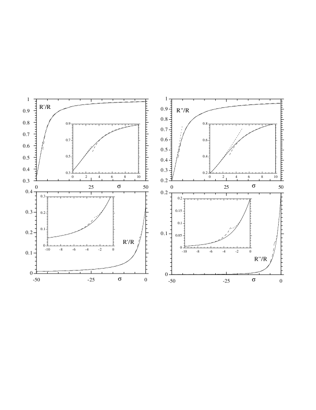
FIGURE 34.: The functions $R^{\prime}/R$ and $R^{\prime\prime}/R$ together with their small and large $\sigma$ approximations. The continuous lines represent the exact functions. Long dashes: large $|\sigma|$ approximations (A.28) and (b). Short dashes: small $\sigma$ approximations (a). The insets show the details of the zones where the small $\sigma$ approximation might be swapped by the corresponding large $\sigma$ approximation, without a significant loss of accuracy.

We can now derive the combinations of $R(\sigma)$ and its derivatives that are required in the main text to construct approximate formulae for various quantities. For $\sigma\ll-1$, these are:

$$\frac{R^{\prime}}{R}\simeq-\frac{1}{2\sigma}\;,\qquad\bigg{(}\frac{R^{\prime}}{R}\bigg{)}^{2}\simeq\frac{1}{4\sigma^{2}}\;,\qquad\frac{R^{\prime\prime}}{R}\simeq\frac{3}{4\sigma^{2}}\;,$$ (A.28)

and the combinations

$$\frac{1}{2}\left[\frac{1}{3}\frac{R^{\prime\prime}}{R}-\bigg{(}\frac{R^{\prime}}{R}\bigg{)}^{2}\right] \simeq 0\;,$$

$$\frac{1}{2}\left[\bigg{(}\frac{R^{\prime}}{R}\bigg{)}^{2}-\frac{R^{\prime\prime}}{R}\right] \simeq -\frac{1}{4\sigma^{2}}\;,$$ (A.29)

$$\frac{1}{16}\left[-1+2\frac{R^{\prime}}{R}-2\bigg{(}\frac{R^{\prime}}{R}\bigg{)}^{2}+\frac{R^{\prime\prime}}{R}\right] \simeq -\frac{1}{16}\left(1+\frac{1}{\sigma}-\frac{1}{4\sigma^{2}}\right)\;.$$

Similarly, for $\sigma\gg 1$ we find

$$\frac{R^{\prime}}{R} \simeq 1-\frac{1}{\sigma}-\frac{1}{2\sigma^{2}}-\frac{5}{4\sigma^{3}}\;,$$

$$\bigg{(}\frac{R^{\prime}}{R}\bigg{)}^{2} \simeq 1-\frac{2}{\sigma}-\frac{3}{2\sigma^{3}}\;,$$ (A.30)

$$\frac{R^{\prime\prime}}{R} \simeq 1-\frac{2}{\sigma}+\frac{1}{\sigma^{2}}-\frac{1}{2\sigma^{3}}\;,$$

and their combinations

$$\frac{1}{2}\left[\frac{1}{3}\frac{R^{\prime\prime}}{R}-\bigg{(}\frac{R^{\prime}}{R}\bigg{)}^{2}\right] \simeq -\frac{1}{3}\left(1-\frac{2}{\sigma}-\frac{1}{2\sigma^{2}}-\frac{2}{\sigma^{3}}\right)\;,$$

$$\frac{1}{2}\left[\bigg{(}\frac{R^{\prime}}{R}\bigg{)}^{2}-\frac{R^{\prime\prime}}{R}\right] \simeq -\left(\frac{1}{2\sigma^{2}}+\frac{1}{2\sigma^{3}}\right)\;,$$ (A.31)

$$\frac{1}{16}\left[-1+2\frac{R^{\prime}}{R}-2\bigg{(}\frac{R^{\prime}}{R}\bigg{)}^{2}+\frac{R^{\prime\prime}}{R}\right] \simeq 0\;.$$

We also write down the leading terms in the $|\sigma|\ll 1$ and $|\sigma|\gg 1$ expansions of the combination $R^{\prime\prime}/R-(R^{\prime}/R)^{2}$, which occurs in some expressions studied in Sections III and IV,

$$\frac{R^{\prime\prime}}{R}-\left(\frac{R^{\prime}}{R}\right)^{2}\simeq\left\{\begin{array}[]{cl}1/2\sigma^{2}&\mbox{ for }\sigma\ll-1\\ 4/45&\mbox{ for }|\sigma|\ll 1\\ 1/\sigma^{2}&\mbox{ for }\sigma\gg 1\end{array}\right.\;.$$ (A.32)

The appropriate combination of Eqs. (a), (A.28), and (b) almost patch the corresponding exact curves over the entire $\sigma$-range. This is shown in Fig. 34, where it can be seen that the use of the $|\sigma|\ll 1$ results, swapped at some point between $|\sigma|=2$ and $|\sigma|=5$ by the corresponding $|\sigma|\gg 1$ formulae, is a reasonable approximation of the exact functions.

Appendix B Derivation of the formulae for the relaxation times

In this appendix we shall give demonstrations of the formulae (5.66) and (5.71) for the relaxation times.

B.1 Integral relaxation time

a The integral relaxation time and the low-frequency dynamical susceptibility

The integral relaxation time defined by Eq. (5.64) is expressible in terms of the eigenvalues, $\Lambda_{k}$, and amplitudes, $a_{k}$, of the Sturm–Liouville problem associated with the axially symmetric Fokker–Planck equation [Eq. (5.65)]. In addition, $\tau_{\rm int}$ can also be written in terms of the low-frequency dynamical susceptibility (Garanin, Ishchenko, and Panina, 1990; Garanin, 1996). In order to show this, let us first write down the general result from linear-response theory

$$\chi(\omega)=\chi-i\omega\int_{0}^{\infty}\!\!{\rm d}{t}\,e^{-i\omega t}\frac{\left\langle m(\infty)\right\rangle-\left\langle m(t)\right\rangle}{\Delta B}\;,$$ (B.1)

where $m(t)$ is the relaxing quantity, $\chi(\omega)$ is its susceptibility counterpart ($\chi$ being the equilibrium susceptibility), and $\Delta B$ is the infinitesimal change in the external control parameter. On applying this result to $\langle m_{z}(\infty)\rangle-\langle m_{z}(t)\rangle$ from Eq. (5.61) and using the sum rule $\sum_{k\geq 1}a_{k}=1$, one finds

$$\chi_{\|}(\omega)=\chi_{\|}\sum_{k\geq 1}a_{k}\bigg{\{}1-i\omega\int_{0}^{\infty}\!\!{\rm d}{t}\,\exp\left[-(i\omega+\Lambda_{k})t\right]\bigg{\}}\;,$$

from which it follows

$$\chi_{\|}(\omega)=\chi_{\|}\sum_{k\geq 1}\frac{a_{k}}{1+i\omega\Lambda_{k}^{-1}}\;.$$ (B.2)

Thus, each exponential mode in the relaxation curve (5.61) gives a Debye-type factor in $\chi_{\|}(\omega)$ weighted by $a_{k}$ and with characteristic time $\Lambda_{k}^{-1}$. Finally, on expanding $\chi_{\|}(\omega)$ for low frequencies by dint of the binomial formula, one gets

$$\chi_{\|}(\omega)\simeq\chi_{\|}\sum_{k\geq 1}a_{k}\left(1-i\omega\Lambda_{k}^{-1}+\cdots\right)=\chi_{\|}\left(1-i\omega\tau_{\rm int}+\cdots\right)\;,$$ (B.3)

where we have again used $\sum_{k\geq 1}a_{k}=1$ and taken Eq. (5.65) into account. Equation (B.3) demonstrates that the calculation of $\tau_{\rm int}$ can effectively be reduced to the calculation of the low-frequency dynamical susceptibility.

b Perturbational solution of the Fokker–Planck equation in the presence of a low sinusoidal field

In order to calculate $\chi_{\|}(\omega)$ one applies a low sinusoidal field, $\Delta\xi(t)=\Delta\xi\exp(i\omega t)$ where $\Delta\xi=m\Delta B/k_{{\rm B}}T$, along the $z$ (symmetry) axis and then calculates the solution of the axially symmetric Fokker–Planck equation (5.47) in such a situation. Since $-\beta{\cal H}(z,t)=-\beta{\cal H}_{0}(z)+z\Delta\xi(t)$, where ${\cal H}_{0}$ is the unperturbed Hamiltonian, we shall seek for a solution for the probability distribution in the stationary regime of the form

$$P(z,t)=P_{{\rm e}}(z)[1+q(z)\Delta\xi(t)]\;,$$ (B.4)

where $P_{{\rm e}}={\cal Z}_{0}^{-1}\exp(-\beta{\cal H}_{0})$ is the equilibrium probability distribution in the absence of the oscillating field.

On introducing the above $P(z,t)$ into the Fokker–Planck equation (5.47) one gets, to first order in $\Delta\xi$ (linear response regime), the following second-order differential equation for $q(z)$

$$\left(-\beta{\cal H}_{0}^{\prime}+\frac{{\rm d}{}}{{\rm d}z}\right)\left[\Omega(z)\frac{{\rm d}q}{{\rm d}z}\right]-i\omega 2\tau_{{\rm N}}q=-\Omega(z)\beta{\cal H}_{0}^{\prime}+\Omega^{\prime}\;,$$ (B.5)

where $\Omega(z)=1-z^{2}$ and the primes denote differentiation with respect to $z$. On the other hand, by taking the introduced form of $P(z,t)$ into account, the non-equilibrium average of the $z$ component of magnetic moment can be written as

$$\left\langle m_{z}(t)\right\rangle=\int_{-1}^{1}\!\!{\rm d}{z}\,P(z,t)m_{z}=m\left\langle z\right\rangle_{{\rm e}}+m\Delta\xi(t)\int_{-1}^{1}\!\!{\rm d}{z}\,P_{{\rm e}}(z)q(z)z\;,$$

where $\langle z\rangle_{{\rm e}}=\int_{-1}^{1}\!\!{\rm d}{z}\,P_{{\rm e}}(z)z$ is the equilibrium average in the unperturbed case. Next, since $\Delta\xi(t)=(m\Delta B/k_{{\rm B}}T)\exp(i\omega t)$, the dynamical susceptibility, which is the coefficient of $\mu_{0}^{-1}\Delta Be^{i\omega t}$ in $\langle m_{z}(t)\rangle$, is given by

$$\chi_{\|}(\omega)=\frac{\mu_{0}m^{2}}{k_{{\rm B}}T}\int_{-1}^{1}\!\!{\rm d}{z}\,P_{{\rm e}}(z)q(z)z\;.$$ (B.6)

Comparison of this equation with Eq. (B.3) reveals that only the low-frequency part of $q(z)$ is required to calculate $\tau_{\rm int}$. This is important since Eq. (B.5) cannot be solved analytically in the general case. In contrast, it can be solved perturbatively for low $\omega$ because, for $\omega=0$, only $q^{\prime}(z)$ and $q^{\prime\prime}(z)$ occur in that equation. This enables one to low the order of the differential equation (B.5) by introducing an auxiliary function $g(z)=q^{\prime}(z)$, and solving successively the system of first-order differential equations for $q(z)$ and $g(z)$.

Let us accomplish this. First, one introduces the perturbational expansion

$$q(z)=q_{0}(z)-(i\omega)q_{1}(z)+(i\omega)^{2}q_{2}(z)-\cdots\;,$$

into Eq. (B.6), getting

$$\chi_{\|}(\omega)=\frac{\mu_{0}m^{2}}{k_{{\rm B}}T}\int_{-1}^{1}\!\!{\rm d}{z}\,P_{{\rm e}}(z)q_{0}(z)z-i\omega\frac{\mu_{0}m^{2}}{k_{{\rm B}}T}\int_{-1}^{1}\!\!{\rm d}{z}\,P_{{\rm e}}(z)q_{1}(z)z+\cdots$$

Then, on comparing this result with Eq. (B.3), one obtains the following integral representation of $\tau_{\rm int}$:

$$\tau_{\rm int}=\frac{1}{\partial\left\langle z\right\rangle_{{\rm e}}/\partial\xi}\int_{-1}^{1}\!\!{\rm d}{z}\,P_{{\rm e}}(z)q_{1}(z)z\;,$$ (B.7)

where we have used $\chi_{\|}=(\mu_{0}m^{2}/k_{{\rm B}}T)\partial\left\langle z\right\rangle_{{\rm e}}/\partial\xi$ [cf. Eqs. (3.59) and (3.60); we can differentiate with respect to $B$ since this is parallel to the probing field $\Delta B$]. Equation (B.7) shows that the calculation of $\tau_{\rm int}$ effectively reduces to that of $q_{1}(z)$. In order to obtain this quantity, we introduce the above perturbational expansion of $q(z)$, along with $g_{i}\equiv{\rm d}q_{i}/{\rm d}z$, into Eq. (B.5), getting

$$\left(-\beta{\cal H}_{0}^{\prime}+\frac{{\rm d}{}}{{\rm d}z}\right)\left\{\Omega(z)[g_{0}-(i\omega)g_{1}+(i\omega)^{2}g_{2}-\cdots]\right\}$$

$$-i\omega 2\tau_{{\rm N}}[q_{0}-(i\omega)q_{1}+\cdots]=-\Omega(z)\beta{\cal H}_{0}^{\prime}+\Omega^{\prime}\;.$$ (B.8)

The zeroth-order equation has the thermal equilibrium solution

$$q_{0}=z-\left\langle z\right\rangle_{{\rm e}}\;,$$ (B.9)

as can be shown by using the definition of $q(z)$ and expanding the equilibrium probability distribution associated with $\beta{\cal H}=\beta{\cal H}_{0}-z\Delta\xi$ [i.e., the $\omega=0$ limit of $\beta{\cal H}(t)$] in powers of $\Delta\xi$.

The $(i\omega)$-order term of Eq. (b) reads

$$\left(-\beta{\cal H}_{0}^{\prime}+\frac{{\rm d}{}}{{\rm d}z}\right)\left[\Omega(z)g_{1}\right]+2\tau_{{\rm N}}q_{0}=0\;.$$

This differential equation can be integrated by quadratures yielding

$$g_{1}(z)=\frac{2\tau_{{\rm N}}}{\Omega(z)}\exp[\beta{\cal H}_{0}(z)]\left[c_{1}+{\cal Z}_{0}\Phi(z)\right]\;,$$ (B.10)

where ${\cal Z}_{0}$ is the (unperturbed) equilibrium partition function and $\Phi(z)$ is given by

$$\Phi(z)=\int_{-1}^{z}{\rm d}z_{1}P_{{\rm e}}(z_{1})\underbrace{(\left\langle z\right\rangle_{{\rm e}}-z_{1})}_{-q_{0}(z_{1})}\;.$$ (B.11)

On using the condition $J_{z}|_{z=\pm 1}=0$ (which follows from the tangency of the current of probability to the unit sphere) and $\Phi(-1)=\Phi(1)=0$ (which immediately follow from the above definition), one gets for the integration constant $c_{1}=0$. Consequently, $q_{1}(z)=\int^{z}\!{\rm d}{z_{2}}\,g_{1}(z_{2})$ is given by

$$q_{1}(z)=c_{2}+2\tau_{{\rm N}}\int_{-1}^{z}\frac{{\rm d}z_{2}}{\Omega(z_{2})}\Phi(z_{2})/P_{{\rm e}}(z_{2})\equiv c_{2}+\tilde{q}_{1}\;,$$ (B.12)

where we have written ${\cal Z}_{0}\exp[\beta{\cal H}_{0}(z_{2})]=1/P_{{\rm e}}(z_{2})$. The new integration constant, $c_{2}$, can be obtained by solving the $(i\omega)^{2}$-order equation and imposing anew the aforementioned condition on the current of probability at the boundaries. On doing so, one finds $c_{2}=-\left\langle\tilde{q}_{1}\right\rangle_{{\rm e}}=-\int_{-1}^{1}\!\!{\rm d}{z}\,P_{{\rm e}}(z)\tilde{q}_{1}(z)$, where $\tilde{q}_{1}(z)$ is the integral term in Eq. (B.12).

c The Garanin, Ishchenko, and Panina formula

We can already do the integral involving $q_{1}(z)$ in the formula (B.7) for the integral relaxation time:

$$\int_{-1}^{1}\!\!{\rm d}{z}\,P_{{\rm e}}(z)q_{1}(z)z = \int_{-1}^{1}\!\!{\rm d}{z}\,P_{{\rm e}}(z)\left[\tilde{q}_{1}(z)-\left\langle\tilde{q}_{1}\right\rangle_{{\rm e}}\right]z$$

$$= \int_{-1}^{1}\!\!{\rm d}{z}\,P_{{\rm e}}(z)\tilde{q}_{1}(z)z-\left\langle z\right\rangle_{{\rm e}}\underbrace{\int_{-1}^{1}\!\!{\rm d}{z}\,P_{{\rm e}}(z)\tilde{q}_{1}(z)}_{\left\langle\tilde{q}_{1}\right\rangle_{{\rm e}}}$$

$$= -\int_{-1}^{1}\underbrace{{\rm d}zP_{{\rm e}}(z)\left(\left\langle z\right\rangle_{{\rm e}}-z\right)}_{{\rm d}\Phi(z){\rm~{}by~{}Eq.~{}(\ref{Phi:2})}}\tilde{q}_{1}(z)$$

$$= -\underbrace{\left[\Phi(z)\tilde{q}_{1}(z)\right]_{-1}^{1}}_{0{\rm~{}by~{}}\Phi(-1)=\Phi(1)=0}+\int_{-1}^{1}\!\!{\rm d}{z}\,\Phi(z)\underbrace{\frac{2\tau_{{\rm N}}}{\Omega(z)}\Phi(z)/P_{{\rm e}}(z)}_{\tilde{q}_{1}^{\prime}(z){\rm~{}by~{}Eq.~{}(\ref{q1})}}\;.$$

Then, on introducing this result into Eq. (B.7) one obtains

$$\tau_{\rm int}=\frac{2\tau_{{\rm N}}}{\partial\left\langle z\right\rangle_{{\rm e}}/\partial\xi}\int_{-1}^{1}\frac{{\rm d}z}{\Omega(z)}\Phi(z)^{2}/P_{{\rm e}}(z)\;,$$ (B.13)

whence, on recalling that $\Omega(z)$ is a shorthand for $1-z^{2}$, one finally gets the result (5.66) of Garanin, Ishchenko, and Panina (1990).

d Explicit expressions for $\Phi(z)$

Let us conclude with the calculation of explicit expressions for $\Phi(z)$ for particular forms of the Hamiltonian. Let us assume that ${\cal H}_{0}$ comprises a uniaxial anisotropy term, $-Kvz^{2}$, plus a Zeeman term, $-mBz$, i.e., $-\beta{\cal H}_{0}=\sigma z^{2}+\xi z$ [see Eq. (2.3)].

1. Isotropic case.

When $\sigma=0$, the equilibrium probability distribution is given by Eq. (2.18). Thus, one of the contributions to $\Phi(z)$ is

$$\left\langle z\right\rangle_{{\rm e}}\int_{-1}^{z}\!\!{\rm d}{z_{1}}\,P_{{\rm e}}(z_{1})=L(\xi)\frac{e^{\xi z}-e^{-\xi}}{2\sinh\xi}\;,$$

where we have used $\langle z\rangle_{{\rm e}}=L(\xi)$, $L(\xi)$ being the Langevin function. The remainder contribution to $\Phi(z)$ is

$$-\int_{-1}^{z}\!\!{\rm d}{z_{1}}\,P_{{\rm e}}(z_{1})z_{1} = -\frac{\xi}{2\sinh\xi}\,\frac{\partial{}}{\partial\xi}\int_{-1}^{z}\!\!{\rm d}{z_{1}}\,\exp(\xi z_{1})$$

$$= -\frac{e^{\xi z}}{2\sinh\xi}\left[\left(z-\frac{1}{3}\right)+e^{-\xi(1+z)}\left(1+\frac{1}{\xi}\right)\right]\;.$$

On adding these two contributions and recalling the definition (2.49) of the Langevin function, one finally gets the explicit result

$$\Phi_{{\rm Lan}}(z)=\frac{P_{{\rm e}}(z)}{\xi}\left[\coth\xi-z-\frac{\exp(-\xi z)}{\sinh\xi}\right]\;.$$ (B.14)

2. Zero-field case.

For $\xi=0$ the equilibrium probability distribution is given by Eq. (2.21). Therefore, $\langle z\rangle_{{\rm e}}=0$ and

$$\Phi(z)=-\frac{1}{2R(\sigma)}\int_{-1}^{z}\!\!{\rm d}{z_{1}}\,\exp(\sigma z_{1}^{2})z_{1}\;.$$

Then, on expressing the result of the integral in terms of the probability distribution (2.21), one gets [note that $P_{{\rm e}}(-1)=P_{{\rm e}}(1)$]

$$\Phi_{{\rm unb}}(z)=\frac{1}{2\sigma}\left[P_{{\rm e}}(1)-P_{{\rm e}}(z)\right]\;.$$ (B.15)

B.2 Effective transverse relaxation time

We shall now derive Eq. (5.71) for the effective transverse relaxation time by performing the low-frequency expansion of the formula for $\chi_{\perp}(\omega)$ of Raĭkher and Shliomis (1975; 1994).

a The Raĭkher and Shliomis formula for the transverse dynamical susceptibility

The expression for $\chi_{\perp}(\omega)$ derived by these authors can be written as

$$\chi_{\perp}(\omega,T)=\chi_{\perp}(T)\frac{\lambda_{a}(\lambda_{b}+i\omega 2\tau_{{\rm N}})+\lambda_{c}}{(\lambda_{1}+i\omega 2\tau_{{\rm N}})(\lambda_{2}+i\omega 2\tau_{{\rm N}})}\;,$$ (B.16)

where $\chi_{\perp}(T)$ is the equilibrium transverse susceptibility (3.53). The coefficients $\lambda_{a}$, $\lambda_{b}$, and $\lambda_{c}$ are given, in terms of the functions $R^{(\ell)}(\sigma)$ [Eq. (2.33)] and the dimensionless damping coefficient $\lambda$ in the Landau–Lifshitz equation, by

$$\lambda_{a}=\frac{R+R^{\prime}}{R-R^{\prime}}\;,\qquad\lambda_{b}=\frac{R-3R^{\prime}+4R^{\prime\prime}}{R^{\prime}-R^{\prime\prime}}\;,\qquad\lambda_{c}=\frac{2\sigma}{\lambda^{2}}\frac{3R^{\prime}-R}{R-R^{\prime}}\;,$$

whereas $\lambda_{1}$ and $\lambda_{2}$ are the roots of the second-degree equation $x^{2}-(\lambda_{a}+\lambda_{b})x+(\lambda_{a}\lambda_{b}+\lambda_{c})=0$. On using that the roots $x_{1}$ and $x_{2}$ of $ax^{2}+bx+c=0$ obey $x_{1}+x_{2}=-(b/a)$ and $x_{1}x_{2}=c/a$, we can write the expression in denominator of $\chi_{\perp}(\omega)$ in terms of $\lambda_{a}$, $\lambda_{b}$, and $\lambda_{c}$ as

$$(\lambda_{1}+i\omega 2\tau_{{\rm N}})(\lambda_{2}+i\omega 2\tau_{{\rm N}})=(\lambda_{a}\lambda_{b}+\lambda_{c})-4\omega^{2}\tau_{{\rm N}}^{2}+i\omega 2\tau_{{\rm N}}(\lambda_{a}+\lambda_{b})\;.$$

Accordingly, the transverse susceptibility (B.16) can equivalently be written as

$$\chi_{\perp}(\omega,T)=\chi_{\perp}(T)\frac{{\displaystyle 1+i\omega 2\tau_{{\rm N}}\frac{\lambda_{a}}{\lambda_{a}\lambda_{b}+\lambda_{c}}}}{{\displaystyle 1-4\omega^{2}\tau_{{\rm N}}^{2}\frac{1}{\lambda_{a}\lambda_{b}+\lambda_{c}}+i\omega 2\tau_{{\rm N}}\frac{\lambda_{a}+\lambda_{b}}{\lambda_{a}\lambda_{b}+\lambda_{c}}}}\;.$$ (B.17)

b Low-frequency expansion of $\chi_{\perp}(\omega)$ and the effective transverse relaxation time

On expanding $\chi_{\perp}(\omega)$ from (B.17) in powers of $\omega\tau_{{\rm N}}$ to first order, we get the simple result

$$\chi_{\perp}(\omega,T)/\chi_{\perp}(T)\simeq 1-i\omega 2\tau_{{\rm N}}\frac{\lambda_{b}}{\lambda_{a}\lambda_{b}+\lambda_{c}}\simeq\frac{1}{{\displaystyle 1+i\omega 2\tau_{{\rm N}}\frac{\lambda_{b}}{\lambda_{a}\lambda_{b}+\lambda_{c}}}}\;,$$ (B.18)

where the last approximate equality has been obtained by means of the binomial expansion $(1+x)^{\epsilon}=1+\epsilon x+\cdots$. Therefore, in the low-frequency range $\chi_{\perp}(\omega)$ has a Debye-type form, so that the quantity multiplying $i\omega$ defines an effective relaxation time, namely

$$\tau_{\perp}|_{\xi=0}=2\tau_{{\rm N}}\frac{1}{\lambda_{a}}\frac{1}{1+\lambda_{c}/\lambda_{a}\lambda_{b}}\;.$$ (B.19)

To conclude, with help from the results of Appendix A, let us write the coefficients $\lambda_{a}$, $\lambda_{b}$, and $\lambda_{c}$ in terms of $\tilde{S}_{2}$ [the average of the second Legendre polynomial (3.73) at zero field]

$$\lambda_{a}=\frac{2+\tilde{S}_{2}}{1-\tilde{S}_{2}}\;,\qquad\lambda_{b}=\frac{2\sigma}{3}\frac{2+\tilde{S}_{2}(1-6/\sigma)}{\tilde{S}_{2}}\;,\qquad\lambda_{c}=\frac{1}{\lambda^{2}}\frac{6\sigma\tilde{S}_{2}}{1-\tilde{S}_{2}}\;,$$

From these equations we get

$$\frac{1}{\lambda_{a}}=\frac{1-\tilde{S}_{2}}{2+\tilde{S}_{2}}\;,\qquad\frac{\lambda_{c}}{\lambda_{a}\lambda_{b}}=\frac{1}{\lambda^{2}}\frac{(3\tilde{S}_{2})^{2}}{(2+\tilde{S}_{2})\big{[}2+\tilde{S}_{2}(1-6/\sigma)\big{]}}\;,$$

which when inserted in Eq. (B.19) yield the effective transverse relaxation time (5.71).

Note finally that, as introduced, the effective transverse relaxation time is a sort of transverse integral relaxation time $\tau_{{\rm int},\perp}$ [compare the first approximate equality of Eq. (B.18) with Eq. (B.3)]. However, its usefulness is questionable in the transverse-field case as the magnetization relaxation curve then comprises oscillating terms, so that the area under such a curve may largely overestimate the relaxation rate.

Appendix C Reduced equations of motion for non-linear system-environment couplings

In this appendix we shall derive a reduced equation of motion for any dynamical variable $A(p,q)$ whose time evolution is determined by the Hamiltonian (6.40). This will be carried out by means of a perturbational expansion in the coupling parameter $\varepsilon$. Nevertheless, we shall first study the weak-coupling dynamics associated with a larger class of Hamiltonians of the form

$${\cal H}_{\rm T}={\cal H}^{({\rm m})}(p,q)+\sum_{\alpha}{\textstyle\frac{1}{2}}\left(P_{\alpha}^{2}+\omega_{\alpha}^{2}Q_{\alpha}^{2}\right)+\varepsilon\sum_{N}{\cal B}^{N}({\bf Q})F_{N}(p,q)\;,$$ (C.1)

where the coupling terms ${\cal B}^{N}({\bf Q})$ are arbitrary functions of the environment coordinates ${\bf Q}$ and $N$ stands for a general index, which can run, for example, over single oscillator indices, pairs, triplets, etc. (${\alpha},{\alpha\beta},{\alpha\beta\gamma},\ldots$). On the other hand, the modified system Hamiltonian ${\cal H}^{({\rm m})}$ augments the system Hamiltonian ${\cal H}$ by appropriate counter-terms, which will be determined below.

We shall first derive the reduced dynamical equations associated with the Hamiltonian (C.1), so that one could incorporate relaxation mechanisms involving any number of environmental normal modes into the dynamical equations of the system variables. This will be done by a perturbational treatment that is an extension of the treatment developed by Cortés, West and Lindenberg (1985) to deal with a system-environment coupling linear in the system coordinate [the case $F_{N}(p,q)\propto q$ of the Hamiltonian (C.1)], but otherwise arbitrary in the environment coordinates. Eventually, we shall particularize the results obtained to the Hamiltonian (6.40), which is recovered when:

1. $N$ only runs over single oscillator indices $\alpha$ and pairs $\alpha\beta$.

2. The corresponding coupling terms are ${\cal B}^{\alpha}({\bf Q})=Q_{\alpha}$ and ${\cal B}^{\alpha\beta}({\bf Q})={\textstyle\frac{1}{2}}Q_{\alpha}Q_{\beta}$.

The coupled dynamical equations for $A(p,q)$ and the environment variables associated with the Hamiltonian (C.1) are [cf. Eqs. (6.16) and (6.17)]

$$\frac{{\rm d}A}{{\rm d}t} = \big{\{}A,{\cal H}^{({\rm m})}\big{\}}+\varepsilon\sum_{N}{\cal B}^{N}({\bf Q})\big{\{}A,F_{N}\big{\}}\;,$$ (C.2)

$$\frac{{\rm d}Q_{\alpha}}{{\rm d}t} = P_{\alpha}\;,\quad\frac{{\rm d}P_{\alpha}}{{\rm d}t}=-\omega_{\alpha}^{2}Q_{\alpha}-\varepsilon\sum_{N}{\cal B}_{\alpha}^{N}({\bf Q})F_{N}\;,$$ (C.3)

where we have used the shorthand

$${\cal B}_{\alpha}^{N}=\partial{\cal B}^{N}/\partial Q_{\alpha}\;.$$

Equations (C.3) can formally be integrated, yielding an equation akin to Eq. (6.18) with $F_{\alpha}(t^{\prime})\to\sum_{N}{\cal B}_{\alpha}^{N}[{\bf Q}(t^{\prime})]F_{N}(t^{\prime})$, namely

$$Q_{\alpha}(t)=Q_{\alpha}^{{\rm h}}(t)-\frac{\varepsilon}{\omega_{\alpha}}\int_{t_{0}}^{t}\!\!{\rm d}{t^{\prime}}\,\sin[\omega_{\alpha}(t-t^{\prime})]\sum_{N}{\cal B}_{\alpha}^{N}[{\bf Q}(t^{\prime})]F_{N}(t^{\prime})\;,$$

where the $Q_{\alpha}^{{\rm h}}(t)$ are the solutions (6.19) for the free oscillators and $F_{N}(t^{\prime})=F_{N}[p(t^{\prime}),q(t^{\prime})]$. On integrating by parts in this equation one gets [cf. Eq. (6.20)]

$$Q_{\alpha}(t)=Q_{\alpha}^{{\rm h}}(t)-\varepsilon\sum_{N}\left[D_{\alpha}^{N}({\bf Q};t,t^{\prime})F_{N}(t^{\prime})\right]_{t^{\prime}=t_{0}}^{t^{\prime}=t}+\varepsilon\int_{t_{0}}^{t}\!\!{\rm d}{t^{\prime}}\,\sum_{N}D_{\alpha}^{N}({\bf Q};t,t^{\prime})\frac{{\rm d}F_{N}}{{\rm d}t}(t^{\prime})\;,$$ (C.4)

where we have introduced the indefinite integral

$$D_{\alpha}^{N}({\bf Q};t,t^{\prime})=\frac{1}{\omega_{\alpha}}\int^{t^{\prime}}\!\!{\rm d}{t^{\prime\prime}}\,\sin[\omega_{\alpha}(t-t^{\prime\prime})]{\cal B}_{\alpha}^{N}[{\bf Q}(t^{\prime\prime})]\;.$$ (C.5)

Recall that writing $Q_{\alpha}(t)$ in the form (C.4) by an integration by parts, enables one to separate the Hamiltonian (renormalization) and relaxational terms (Subsec. VI.C). However, Eq. (C.4) gives $Q_{\alpha}(t)$ in implicit form, since $Q_{\alpha}(t)$ also appears on the right-hand side via ${\cal B}_{\alpha}^{N}({\bf Q})$. Thus, Eq. (C.4) is an explicit solution only in the linear ${\cal B}^{N}({\bf Q})$ case of the Hamiltonian (6.14).

For weak system-environment interactions, we shall solve Eq. (C.4) for $Q_{\alpha}(t)$ perturbatively in $\varepsilon$. However, as pointed out by Cortés, West and Lindenberg (1985), in order to get eventually a thermodynamically consistent description, the expansion cannot be uniform in $\varepsilon$. If one keeps fluctuating terms up to order $\varepsilon^{k}$, the relaxation terms must be retained up to order $\varepsilon^{2k}$, in order to obtain proper fluctuation-dissipation relations [see, for example, Eqs. (6.28), (6.30) and (6.38)].

The $\varepsilon$-expansion of $Q_{\alpha}(t)$ reads

$$Q_{\alpha}(t)=Q_{\alpha}^{{\rm h}}(t)+\varepsilon\,\delta Q_{\alpha}(t)+\ldots\;,$$

where $\varepsilon\,\delta Q_{\alpha}(t)$ is given by the second plus third terms on the right-hand side of Eq. (C.4) when ${\bf Q}^{{\rm h}}$ (the zeroth-order term) is substituted for ${\bf Q}$ in $D_{\alpha}^{N}({\bf Q};t,t^{\prime})$, namely

$$\varepsilon\,\delta Q_{\alpha}(t)=-\varepsilon\sum_{N}\left[D_{\alpha}^{N}({\bf Q}^{{\rm h}};t,t^{\prime})F_{N}(t^{\prime})\right]_{t^{\prime}=t_{0}}^{t^{\prime}=t}+\varepsilon\int_{t_{0}}^{t}\!\!{\rm d}{t^{\prime}}\,\sum_{N}D_{\alpha}^{N}({\bf Q}^{{\rm h}};t,t^{\prime})\frac{{\rm d}F_{N}}{{\rm d}t}(t^{\prime})$$

[that is, we iterate Eq. (C.4) into itself]. The corresponding expansion of the coupling functions is given by

$$\varepsilon{\cal B}^{N}({\bf Q})=\varepsilon{\cal B}^{N}({\bf Q}^{{\rm h}})+{\varepsilon}^{2}\sum_{\alpha}{\cal B}_{\alpha}^{N}({\bf Q}^{{\rm h}})\delta Q_{\alpha}+\ldots\;,$$ (C.6)

which enters into Eq. (C.2). The term

$$f_{N}(t)\equiv\varepsilon{\cal B}^{N}[{\bf Q}^{{\rm h}}(t)]\;,$$ (C.7)

per analogy with $f_{\alpha}(t)=\varepsilon Q_{\alpha}^{{\rm h}}(t)$ [Eq. (6.21)], is interpreted as the lowest order fluctuation. Following the programme of Cortés, West and Lindenberg (1985), we shall retain fluctuations only to this order.

Concerning the back-reaction part, one first introduces the quantities

$${\cal K}^{N,M}(t,t^{\prime}) = {\varepsilon}^{2}\Big{\langle}\sum_{\alpha}{\cal B}_{\alpha}^{N}[{\bf Q}^{{\rm h}}(t)]D_{\alpha}^{M}({\bf Q}^{{\rm h}};t,t^{\prime})\Big{\rangle}\;,$$ (C.8)

$$\delta{\cal K}^{N,M}(t,t^{\prime}) = {\varepsilon}^{2}\sum_{\alpha}{\cal B}_{\alpha}^{N}[{\bf Q}^{{\rm h}}(t)]D_{\alpha}^{M}({\bf Q}^{{\rm h}};t,t^{\prime})-{\cal K}^{N,M}(t,t^{\prime})\;,$$ (C.9)

so that the second term in the expansion (C.6) can be decomposed as

$${\varepsilon}^{2}\sum_{\alpha}{\cal B}_{\alpha}^{N}({\bf Q}^{{\rm h}})\delta Q_{\alpha} = -\Big{[}\sum_{M}\left[{\cal K}^{N,M}(t,t^{\prime})+\delta{\cal K}^{N,M}(t,t^{\prime})\right]F_{M}(t^{\prime})\Big{]}_{t^{\prime}=t_{0}}^{t^{\prime}=t}$$

$${}+\int_{t_{0}}^{t}\!\!{\rm d}{t^{\prime}}\,\sum_{M}\left[{\cal K}^{N,M}(t,t^{\prime})+\delta{\cal K}^{N,M}(t,t^{\prime})\right]\frac{{\rm d}F_{M}}{{\rm d}t}(t^{\prime})\;.$$

Each kernel ${\cal K}^{N,M}$ gives a different type of contribution whereas the contribution of $\delta{\cal K}^{N,M}$ can be interpreted as fluctuations around the former (Cortés, West and Lindenberg, 1985). As these fluctuations are of order higher ($\varepsilon^{2}$) than the fluctuations that we are retaining in the present treatment, the terms $\delta{\cal K}^{N,M}$ will henceforth be omitted. On the other hand, the terms $\sum_{M}{\cal K}^{N,M}(t,t_{0})F_{M}(t_{0})$ in ${\varepsilon}^{2}\sum_{\alpha}{\cal B}_{\alpha}^{N}\delta Q_{\alpha}$ will also be ignored as they are the generalization of those terms that give a transient in the response (see Subsec. VI.C; recall however that they could be incorporated into an alternative definition of the fluctuating sources but, as they are of order $\varepsilon^{2}$, they would anyhow be ignored). Finally, the parallel terms $-\sum_{M}{\cal K}^{N,M}(t,t)F_{M}(t)$ give the Hamiltonian contributions. In order to prove this, note first that, since ${\cal K}^{N,M}(t,t^{\prime})$ comprises equilibrium averages, it depends on $(t-t^{\prime})$ and, hence, ${\cal K}^{N,M}(t,t)$ is independent of $t$. By the same reasoning one can demonstrate the symmetry property ${\cal K}^{N,M}={\cal K}^{M,N}$. Then, by using the product rule of the Poisson bracket (6.22), one finds that the contribution originating from $-\sum_{M}{\cal K}^{N,M}(t,t)F_{M}(t)$ in the equation for $A(p,q)$ is given by

$$-\sum_{NM}{\cal K}^{N,M}(0)\big{\{}A,F_{N}\big{\}}F_{M}=\Big{\{}A,-{\textstyle\frac{1}{2}}\sum_{NM}{\cal K}^{N,M}(0)F_{N}F_{M}\Big{\}}\;,$$

which is indeed derivable from a (time-independent) Hamiltonian. This term is associated with the coupling-induced renormalization of the energy of the system and is balanced by the counter-terms incorporated into ${\cal H}^{({\rm m})}$, now explicitly identified as [cf. Eq. (6.15)]

$${\cal H}^{({\rm m})}={\cal H}+{\textstyle\frac{1}{2}}\sum_{NM}{\cal K}^{N,M}(0)F_{N}F_{M}\;.$$ (C.10)

On collecting the terms whose retention has hitherto been argued and introducing them into Eq. (C.2), one finally gets the approximate reduced equation of motion for any dynamical variable $A(p,q)$ [cf. Eq. (6.23)]

$$\frac{{\rm d}A}{{\rm d}t}=\big{\{}A,{\cal H}\big{\}}+\sum_{N}\big{\{}A,F_{N}\big{\}}\bigg{[}f_{N}(t)+\int_{t_{0}}^{t}\!\!{\rm d}{t^{\prime}}\,\sum_{M}{\cal K}^{N,M}(t-t^{\prime})\frac{{\rm d}F_{M}}{{\rm d}t}(t^{\prime})\bigg{]}\;.$$ (C.11)

In addition, within the approximation used (fluctuating and relaxation terms to order $\varepsilon$ and $\varepsilon^{2}$, respectively), one can replace ${\rm d}F_{M}/{\rm d}t$ in the memory integral by its conservative part ${\rm d}F_{M}/{\rm d}t\simeq\big{\{}F_{M},{\cal H}\big{\}}$. On the other hand, one can establish fluctuation-dissipation relations by means of arguments parallel to those presented by Cortés, West and Lindenberg (1985).

To conclude, we shall particularize these results to the linear-plus-quadratic couplings of the Hamiltonian (6.40). This is recovered when $N$ runs over single oscillator indices $\alpha$, with ${\cal B}^{\alpha}=Q_{\alpha}$, and pairs $\alpha\beta$, with ${\cal B}^{\alpha\beta}={\textstyle\frac{1}{2}}Q_{\alpha}Q_{\beta}$. Then, the fluctuating terms $f_{N}(t)=\varepsilon{\cal B}^{N}[{\bf Q}^{{\rm h}}(t)]$ are given by $f_{\alpha}(t)=\varepsilon Q_{\alpha}^{{\rm h}}(t)$ [Eq. (6.21)] and $f_{\alpha\beta}(t)=(\varepsilon/2)Q_{\alpha}^{{\rm h}}(t)Q_{\beta}^{{\rm h}}(t)$ [Eq. (6.43)]. On the other hand, by inserting the derivatives

$${\cal B}_{\gamma}^{\alpha} = \partial{\cal B}^{\alpha}/\partial Q_{\gamma}=\delta_{\alpha\gamma}\;,$$ (C.12)

$${\cal B}_{\gamma}^{\alpha\beta} = \partial{\cal B}^{\alpha\beta}/\partial Q_{\gamma}={\textstyle\frac{1}{2}}(\delta_{\alpha\gamma}Q_{\beta}+\delta_{\beta\gamma}Q_{\alpha})\;,$$ (C.13)

into Eq. (C.5), the functions $D_{\gamma}^{N}({\bf Q};t,t^{\prime})$ emerge in the form ($N=\alpha,\,\alpha\beta$)

$$D_{\gamma}^{\alpha}({\bf Q};t,t^{\prime}) = \frac{\delta_{\alpha\gamma}}{\omega_{\alpha}^{2}}\cos[\omega_{\alpha}(t-t^{\prime})]\;,$$ (C.14)

$$D_{\gamma}^{\alpha\beta}({\bf Q};t,t^{\prime}) = \frac{1}{\omega_{\gamma}}\int^{t^{\prime}}\!\!{\rm d}{t^{\prime\prime}}\,\sin[\omega_{\gamma}(t-t^{\prime\prime})]{\textstyle\frac{1}{2}}[\delta_{\alpha\gamma}Q_{\beta}(t^{\prime\prime})+\delta_{\beta\gamma}Q_{\alpha}(t^{\prime\prime})]\;.\qquad\quad$$ (C.15)

Therefore, on taking the averages in Eq. (C.8) with respect to the distribution (6.35) (decoupled initial conditions) by means of Eqs. (6.36), we get for the kernels ${\cal K}^{N,M}$ (see proofs below)

$${\cal K}^{\alpha,\beta}(\tau) = \delta_{\alpha\beta}\frac{\varepsilon^{2}}{\omega_{\alpha}^{2}}\cos(\omega_{\alpha}\tau)\;,$$ (C.16)

$${\cal K}^{\alpha,\beta\gamma}(\tau) = {\cal K}^{\alpha\beta,\gamma}(\tau)=0\;,$$ (C.17)

$${\cal K}^{\alpha\beta,\gamma\delta}(\tau) = {\textstyle\frac{1}{2}}(\delta_{\alpha\gamma}\delta_{\beta\delta}+\delta_{\alpha\delta}\delta_{\beta\gamma})$$ (C.18)

$${}\times\frac{\varepsilon^{2}}{2}\frac{k_{{\rm B}}T}{2\omega_{\alpha}^{2}\omega_{\beta}^{2}}\big{\{}\cos[(\omega_{\alpha}-\omega_{\beta})\tau]+\cos[(\omega_{\alpha}+\omega_{\beta})\tau]\big{\}}\;.\qquad$$

These kernels satisfy the properties mentioned above: they depend on $\tau=t-t^{\prime}$ and are symmetrical with respect to the indices separated by commas, which correspond to the general indices $N,M$.

On introducing all these results in Eq. (C.11), the resulting dynamical equation for $A(p,q)$ is given by Eq. (6.42). For the sake of simplicity, we have introduced in that equation the kernels ${\cal K}_{\alpha}(\tau)$ and ${\cal K}_{\alpha\beta}(\tau)$, which are defined in terms of the above kernels by

$${\cal K}^{\alpha,\beta}(\tau) = \delta_{\alpha\beta}{\cal K}_{\alpha}(\tau)\;,$$

$${\cal K}^{\alpha\beta,\gamma\delta}(\tau) = {\textstyle\frac{1}{2}}(\delta_{\alpha\gamma}\delta_{\beta\delta}+\delta_{\alpha\delta}\delta_{\beta\gamma}){\cal K}_{\alpha\beta}(\tau)\;.$$

Besides, on explicitly writing the counter-term of Eq. (C.10) in this linear-plus-quadratic case, one arrives at Eq. (6.41).

Note finally that, owing to the fact that ${\cal B}_{\gamma}^{\alpha}({\bf Q}^{{\rm h}})D_{\gamma}^{\beta}({\bf Q}^{{\rm h}};t,t^{\prime})$ does not depend on ${\bf Q}^{{\rm h}}$, the kernel ${\cal K}_{\alpha}(\tau)$ is not affected by the averaging procedure, whereas this renders ${\cal K}_{\alpha\beta}(\tau)$ explicitly dependent on the temperature (see below). In this connection, we remark that the modifications of this last kernel obtained when one assumes coupled initial conditions, begin at order $\varepsilon^{3}$.

Derivation of the kernels

1. Derivation of ${\cal K}^{\alpha,\beta}(\tau)$.

From Eqs. (C.12) and (C.14) and the general definition ${\cal K}^{N,M}(t,t^{\prime})=\varepsilon^{2}\langle\sum_{\rho}{\cal B}_{\rho}^{N}D_{\rho}^{M}\rangle$, one gets

$${\cal K}^{\alpha,\beta}(t,t^{\prime}) = \varepsilon^{2}\Big{\langle}\sum_{\rho}{\cal B}_{\rho}^{\alpha}D_{\rho}^{\beta}\Big{\rangle}$$

$$= \varepsilon^{2}\Big{\langle}\sum_{\rho}\delta_{\alpha\rho}\frac{\delta_{\beta\rho}}{\omega_{\beta}^{2}}\cos[\omega_{\beta}(t-t^{\prime})]\Big{\rangle}=\delta_{\alpha\beta}\frac{\varepsilon^{2}}{\omega_{\alpha}^{2}}\cos[\omega_{\alpha}(t-t^{\prime})]\;,$$

where the average has played no rôle. Q.E.D.

2. Derivation of ${\cal K}^{\alpha,\beta\gamma}(\tau)$.

From Eqs. (C.12) and (C.15) we obtain

$$\left\langle{\cal B}_{\rho}^{\alpha}D_{\rho}^{\beta\gamma}\right\rangle=\frac{\delta_{\alpha\rho}}{\omega_{\rho}}\int^{t^{\prime}}\!\!{\rm d}{t^{\prime\prime}}\,\sin[\omega_{\rho}(t-t^{\prime\prime})]{\textstyle\frac{1}{2}}\Big{[}\delta_{\beta\rho}\underbrace{\left\langle Q_{\gamma}^{{\rm h}}(t^{\prime\prime})\right\rangle}_{0}+\delta_{\gamma\rho}\underbrace{\left\langle Q_{\beta}^{{\rm h}}(t^{\prime\prime})\right\rangle}_{0}\Big{]}=0\;,$$

where Eqs. (6.36) have been employed. Therefore, from this result and the general definition (C.8) it follows that ${\cal K}^{\alpha,\beta\gamma}(t,t^{\prime})=0$. Q.E.D.

3. Derivation of ${\cal K}^{\alpha\beta,\gamma}(\tau)$.

The average of the product of Eqs. (C.13) and (C.14) evaluated at ${\bf Q}^{{\rm h}}$ is zero as well. Indeed,

$$\left\langle{\cal B}_{\rho}^{\alpha\beta}D_{\rho}^{\gamma}\right\rangle={\textstyle\frac{1}{2}}\Big{[}\delta_{\alpha\rho}\underbrace{\left\langle Q_{\beta}^{{\rm h}}(t)\right\rangle}_{0}+\delta_{\beta\rho}\underbrace{\left\langle Q_{\alpha}^{{\rm h}}(t)\right\rangle}_{0}\Big{]}\frac{\delta_{\gamma\rho}}{\omega_{\gamma}^{2}}\cos[\omega_{\gamma}(t-t^{\prime})]=0\;,$$

whence one gets the stated result ${\cal K}^{\alpha\beta,\gamma}(t,t^{\prime})=0$. Q.E.D.

4. Derivation of ${\cal K}^{\alpha\beta,\gamma\delta}(\tau)$.

Finally, for the average of the product of Eqs. (C.13) and (C.15) evaluated at ${\bf Q}^{{\rm h}}$ one has

$$\left\langle{\cal B}_{\rho}^{\alpha\beta}D_{\rho}^{\gamma\delta}\right\rangle$$

$$=\Big{\langle}{\textstyle\frac{1}{2}}\big{[}\delta_{\alpha\rho}Q_{\beta}^{{\rm h}}(t)+\delta_{\beta\rho}Q_{\alpha}^{{\rm h}}(t)\big{]}$$

$$\qquad{}\times\frac{1}{\omega_{\rho}}\int^{t^{\prime}}\!\!{\rm d}{t^{\prime\prime}}\,\sin[\omega_{\rho}(t-t^{\prime\prime})]{\textstyle\frac{1}{2}}\big{[}\delta_{\gamma\rho}Q_{\delta}^{{\rm h}}(t^{\prime\prime})+\delta_{\delta\rho}Q_{\gamma}^{{\rm h}}(t^{\prime\prime})\big{]}\Big{\rangle}\;.$$

Therefore, we need to calculate the following average

$$\Big{\langle}\big{[}\delta_{\alpha\rho}Q_{\beta}^{{\rm h}}(t)+\delta_{\beta\rho}Q_{\alpha}^{{\rm h}}(t)\big{]}\big{[}\delta_{\gamma\rho}Q_{\delta}^{{\rm h}}(t^{\prime\prime})+\delta_{\delta\rho}Q_{\gamma}^{{\rm h}}(t^{\prime\prime})\big{]}\Big{\rangle}$$

$$= k_{{\rm B}}T\bigg{\{}\delta_{\alpha\rho}\delta_{\gamma\rho}\frac{\delta_{\beta\delta}}{\omega_{\beta}^{2}}\cos[\omega_{\beta}(t-t^{\prime\prime})]+\delta_{\alpha\rho}\delta_{\delta\rho}\frac{\delta_{\beta\gamma}}{\omega_{\beta}^{2}}\cos[\omega_{\beta}(t-t^{\prime\prime})]$$

$$\qquad\quad{}+\delta_{\beta\rho}\delta_{\gamma\rho}\frac{\delta_{\alpha\delta}}{\omega_{\alpha}^{2}}\cos[\omega_{\alpha}(t-t^{\prime\prime})]+\delta_{\beta\rho}\delta_{\delta\rho}\frac{\delta_{\alpha\gamma}}{\omega_{\alpha}^{2}}\cos[\omega_{\alpha}(t-t^{\prime\prime})]\bigg{\}}$$

$$= \frac{k_{{\rm B}}T}{\omega_{\alpha}^{2}\omega_{\beta}^{2}}\Big{\{}\delta_{\alpha\rho}(\delta_{\gamma\rho}\delta_{\beta\delta}+\delta_{\delta\rho}\delta_{\beta\gamma})\omega_{\alpha}^{2}\cos[\omega_{\beta}(t-t^{\prime\prime})]$$

$$\qquad\quad{}+\delta_{\beta\rho}(\delta_{\gamma\rho}\delta_{\alpha\delta}+\delta_{\delta\rho}\delta_{\alpha\gamma})\omega_{\beta}^{2}\cos[\omega_{\alpha}(t-t^{\prime\prime})]\Big{\}}\;,$$

where we have used Eqs. (6.36). Next, on multiplying this expression by $\sin[\omega_{\rho}(t-t^{\prime\prime})]/\omega_{\rho}$, and summing over $\rho$ we obtain

$$\sum_{\rho}\Big{\langle}\big{[}\delta_{\alpha\rho}Q_{\beta}^{{\rm h}}(t)+\delta_{\beta\rho}Q_{\alpha}^{{\rm h}}(t)\big{]}\big{[}\delta_{\gamma\rho}Q_{\delta}^{{\rm h}}(t^{\prime\prime})+\delta_{\delta\rho}Q_{\gamma}^{{\rm h}}(t^{\prime\prime})\big{]}\Big{\rangle}\sin[\omega_{\rho}(t-t^{\prime\prime})]/\omega_{\rho}$$

$$= \frac{k_{{\rm B}}T}{\omega_{\alpha}^{2}\omega_{\beta}^{2}}(\delta_{\alpha\gamma}\delta_{\beta\delta}+\delta_{\alpha\delta}\delta_{\beta\gamma})$$

$${}\times\Big{\{}\omega_{\alpha}\cos[\omega_{\beta}(t-t^{\prime\prime})]\sin[\omega_{\alpha}(t-t^{\prime\prime})]+\omega_{\beta}\cos[\omega_{\alpha}(t-t^{\prime\prime})]\sin[\omega_{\beta}(t-t^{\prime\prime})]\Big{\}}\;.$$

Then, on taking into account that $({\rm d}/{\rm d}{t^{\prime\prime}})\{\cos[\omega_{\alpha}(t-t^{\prime\prime})]\cos[\omega_{\beta}(t-t^{\prime\prime})]\}$ is equal to the term within the above curly brackets when calculating the integral occurring in ${\cal K}^{\alpha\beta,\gamma\delta}(t,t^{\prime})=\varepsilon^{2}\langle\sum_{\rho}{\cal B}_{\rho}^{\alpha\beta}D_{\rho}^{\gamma\delta}\rangle$, we arrive at

$${\cal K}^{\alpha\beta,\gamma\delta}(t,t^{\prime})={\textstyle\frac{1}{2}}(\delta_{\alpha\gamma}\delta_{\beta\delta}+\delta_{\alpha\delta}\delta_{\beta\gamma})\frac{\varepsilon^{2}}{2}\frac{k_{{\rm B}}T}{\omega_{\alpha}^{2}\omega_{\beta}^{2}}\cos[\omega_{\alpha}(t-t^{\prime})]\cos[\omega_{\beta}(t-t^{\prime})]\;,$$

whence one immediately obtains Eq. (C.18). Q.E.D.

References

- [1]
- [2] [] Aharoni, A. (1964), Phys. Rev. 135, A447–A449.
- [3]
- [4] [] Arfken, G. (1985), Mathematical Methods for Physicists, 3rd ed., Academic Press, Boston.
- [5]
- [6] [] Barra, A.-L., Debrunner, P., Gatteschi, D., Schultz, C. E. and Sessoli, R. (1996), Europhys. Lett. 35, 133–138.
- [7]
- [8] [] Bessais, L., Ben Jaffel, L. and Dormann, J. L. (1992), Phys. Rev. B 45, 7805–7815.
- [9]
- [10] [] Binder, K. and Stauffer, D. (1984), in Applications of the Monte Carlo Method in Statistical Physics, K. Binder, ed., Springer, Berlin, p. 1.
- [11]
- [12] [] Bitoh, T., Ohba, K., Takamatsu, M., Shirane, T. and Chikazawa, S. (1993), J. Phys. Soc. Jpn. 62, 2583–2586.
- [13]
- [14] [] Bitoh, T., Ohba, K., Takamatsu, M., Shirane, T. and Chikazawa, S. (1995), J. Phys. Soc. Jpn. 64, 1311–1319.
- [15]
- [16] [] Böttcher, C. J. F. and Bordewijk, P. (1978), Theory of Electric Polarization Vol. II, Elsevier, Amsterdam.
- [17]
- [18] [] Brown, Jr., W. F. (1959), J. Appl. Phys. 30, 130s–133s.
- [19]
- [20] [] Brown, Jr., W. F. (1963), Phys. Rev. 130, 1677–1686.
- [21]
- [22] [] Brown, Jr., W. F. (1979), IEEE Trans. Magn. MAG-15, 1196–1208.
- [23]
- [24] [] Brown, Jr., W. F. and Morrish, A. H. (1957), Phys. Rev. 105, 1198–1201.
- [25]
- [26] [] Brun, T. A. (1993), Phys. Rev. D 47, 3383–3393.
- [27]
- [28] [] Caldeira, A. O. and Leggett, A. J. (1983), Ann. Phys. (New York) 149, 374–456.
- [29]
- [30] [] Chantrell, R. W., Ayoub, N. Y. and Popplewell, J. (1985), J. Magn. Magn. Mater. 53, 199–207.
- [31]
- [32] [] Chikazumi, S. (1978), Physics of Magnetism, Krieger, New York.
- [33]
- [34] [] Coffey, W. T. (1998), Adv. Chem. Phys. 103, 259–333.
- [35]
- [36] [] Coffey, W. T., Cregg, P. J. and Kalmykov, Yu. P. (1993), Adv. Chem. Phys. 83, 263–464.
- [37]
- [38] [] Coffey, W. T., Crothers, D. S. F., Kalmykov, Yu. P., Massawe, E. S. and Waldron, J. T. (1994), Phys. Rev. E 49, 1869–1882.
- [39]
- [40] [] Coffey, W. T., Crothers, D. S. F., Kalmykov, Yu. P. and Waldron, J. T. (1995a), Phys. Rev. B 51, 15947–15956.
- [41]
- [42] [] Coffey, W. T., Crothers, D. S. F., Kalmykov, Yu. P. and Waldron, J. T. (1995b), Physica A 213, 551–575.
- [43]
- [44] [] Coffey, W. T., Kalmykov, Yu. P. and Massawe, E. S. (1993), Adv. Chem. Phys. 85, 667–792.
- [45]
- [46] [] Cortés, E., West, B. J. and Lindenberg, K. (1985), J. Chem. Phys. 82, 2708–2717.
- [47]
- [48] [] Cregg, P. J. and Bessais, L. (1999a), J. Magn. Magn. Mater. 202, 554–564.
- [49]
- [50] [] Cregg, P. J. and Bessais, L. (1999b), J. Magn. Magn. Mater. 203, 265–267.
- [51]
- [52] [] Cregg, P. J., Crothers, D. S. F. and Wickstead, A. W. (1994), J. Appl. Phys. 76, 4900–4902.
- [53]
- [54] [] Ettelaie, R. and Moore, M. A. (1984), J. Phys. A 17, 3505–3520.
- [55]
- [56] [] Ford, G. W., Lewis, J. T. and O’Connell, R. F. (1988), Phys. Rev. A 37, 4419–4428.
- [57]
- [58] [] Garanin, D. A. (1996), Phys. Rev. E 54, 3250–3256.
- [59]
- [60] [] Garanin, D. A. (1997), Phys. Rev. B 55, 3050–3057.
- [61]
- [62] [] Garanin, D. A., Ishchenko, V. V. and Panina, L. V. (1990), Theor. Math. Phys. (USSR) 82, 169–179 [Teor. Mat. Fiz. 82, 242 (1990)].
- [63]
- [64] [] García-Palacios, J. L. (1999), Eur. Phys. J. B (in press).
- [65]
- [66] [] García-Palacios, J. L., Jönsson, P. and Svedlindh, P. (1999), (unpublished).
- [67]
- [68] [] García-Palacios, J. L. and Lázaro, F. J. (1997), Phys. Rev. B 55, 1006–1010.
- [69]
- [70] [] García-Palacios, J. L. and Lázaro, F. J. (1998), Phys. Rev. B 58, 14937–14958.
- [71]
- [72] [] Garg, A. and Kim, G.-H. (1991), Phys. Rev. B 43, 712–718.
- [73]
- [74] [] Gekht, R. S. (1983), Phys. Met. Metallogr. (USSR) 55, 12–17 [Fiz. Met. Metalloved. 55, 225 (1983)].
- [75]
- [76] [] Gekht, R. S. and Ignatchenko, V. A. (1979), Sov. Phys. JETP 49, 84–89 [Zh. Eksp. Teor. Fiz. 76, 164 (1979)].
- [77]
- [78] [] Gilbert, T. L. (1955), Phys. Rev. 100, 1243.
- [79]
- [80] [] Gittleman, J. I., Abeles, B. and Bozowski, S. (1974), Phys. Rev. B 9, 3891–3897.
- [81]
- [82] [] Gomes, A. M., Novak, M. A., Sessoli, R., Caneschi, A. and Gatteschi, D. (1998), Phys. Rev. B 57, 5021–5024.
- [83]
- [84] [] Hennion, M., Bellouard, C., Mirebeau, I., Dormann, J. L. and Nogues, M. (1994), Europhys. Lett. 25, 43–48.
- [85]
- [86] [] Jacobs, I. S. and Bean, C. P. (1963), in Magnetism, Vol. III, G. T. Rado and H. Suhl, eds., Academic Press, New York–London, pp. 271–350.
- [87]
- [88] [] Jayannavar, A. M. (1991), Z. Phys. B 82, 153–156.
- [89]
- [90] [] Jonsson, T., Mattsson, J., Djurberg, C., Khan, F. A., Nordblad, P. and Svedlindh, P. (1995), Phys. Rev. Lett. 75, 4138–4141.
- [91]
- [92] [] Jung, P. and Risken, H. (1985), Z. Phys. B 59, 469–481.
- [93]
- [94] [] Kalmykov, Yu. P. and Coffey, W. T. (1997), Phys. Rev. B 56, 3325–3337.
- [95]
- [96] [] Klik, I. (1992), J. Stat. Phys. 66, 635–645.
- [97]
- [98] [] Kloeden, P. E. and Platen, E. (1995), Numerical Solution of Stochastic Differential Equations, 2nd corr. printing, Springer, Berlin.
- [99]
- [100] [] Krueger, D. A. (1979), J. Appl. Phys. 50, 8169–8171.
- [101]
- [102] [] Kubo, R. and Hashitsume, N. (1970), Prog. Theor. Phys. Suppl. 46, 210–220.
- [103]
- [104] [] Landau, L. D. and Lifshitz, E. M. (1935), Z. Phys. Sowjet. 8, 153–169.
- [105]
- [106] [] Landau, L. D. and Lifshitz, E. M. (1980), Statistical Physics (Part 1), 3rd ed., Pergamon Press, Oxford.
- [107]
- [108] [] Landau, L. D. and Lifshitz, E. M. (1984), Electrodynamics of Continuous Media, 2nd ed., Pergamon Press, Oxford.
- [109]
- [110] [] Lin, C. J. (1961), J. Appl. Phys. 32, 233s–234s.
- [111]
- [112] [] Lindenberg, K., Mohanty, U. and Seshadri, V. (1983), Physica A 119, 1–16.
- [113]
- [114] [] Lindenberg, K. and Seshadri, V. (1981), Physica A 109, 483–499.
- [115]
- [116] [] Lindenberg, K. and West, B. J. (1984), Phys. Rev. A 30, 568–582.
- [117]
- [118] [] Lundgren, L., Svedlindh, P. and Beckman, O. (1981), J. Magn. Magn. Mater. 25, 33–38.
- [119]
- [120] [] Luo, W., Nagel, S. R., Rosenbaum, T. F. and Rosensweig, R. E. (1991), Phys. Rev. Lett. 67, 2721–2724.
- [121]
- [122] [] Magalinskiĭ, V. B. (1959), Sov. Phys. JETP 9, 1381–1382 [Zh. Eksp. Teor. Fiz. 36, 1942 (1959)].
- [123]
- [124] [] Maiti, A. and Falicov, L. M. (1993), Phys. Rev. B 48, 13596–13601.
- [125]
- [126] [] Morillo, M. and Gómez-Ordóñez, J. (1993), Phys. Rev. Lett. 71, 9–11.
- [127]
- [128] [] Moro, G. and Nordio, P. L. (1985), Mol. Phys. 56, 255–269.
- [129]
- [130] [] Mørup, S. (1983), J. Magn. Magn. Mater. 37, 39–50.
- [131]
- [132] [] Néel, L. (1949), Ann. Geophys. 5, 99–136.
- [133]
- [134] [] Pérez-Madrid, A. and Rubí, J. M. (1995), Phys. Rev. E 51, 4159–4164.
- [135]
- [136] [] Raĭkher, Yu. L. and Shliomis, M. I. (1975), Sov. Phys. JETP 40, 526–532 [Zh. Eksp. Teor. Fiz. 67, 1060 (1974)].
- [137]
- [138] [] Raĭkher, Yu. L. and Shliomis, M. I. (1994), Adv. Chem. Phys. 87, 595–751.
- [139]
- [140] [] Raĭkher, Yu. L. and Stepanov, V. I. (1994), J. Phys.: Condens. Matter 6, 4137–4145.
- [141]
- [142] [] Raĭkher, Yu. L. and Stepanov, V. I. (1995a), Phys. Rev. B 51, 16428–16431.
- [143]
- [144] [] Raĭkher, Yu. L. and Stepanov, V. I. (1995b), Phys. Rev. B 52, 3493–3498.
- [145]
- [146] [] Raĭkher, Yu. L. and Stepanov, V. I. (1997), Phys. Rev. B 55, 15005–15017.
- [147]
- [148] [] Raĭkher, Yu. L., Stepanov, V. I., Grigorenko, A. N. and Nikitin, P. I. (1997), Phys. Rev. E 56, 6400–6409.
- [149]
- [150] [] Ramírez-Piscina, L., Sancho, J. M. and Hernández-Machado, A. (1993), Phys. Rev. B 48, 125–131.
- [151]
- [152] [] Risken, H. (1989), The Fokker–Planck Equation, 2nd ed., Springer, Berlin.
- [153]
- [154] [] Rodé, D., Bertram, H. N. and Fredkin, D. R. (1987), IEEE Trans. Magn. MAG-23, 2224–2226.
- [155]
- [156] [] Rümelin, W. (1982), SIAM (Soc. Ind. Appl. Math.) J. Numer. Anal. 19, 604–613.
- [157]
- [158] [] Sadykov, E. K. (1992), J. Phys.: Condens. Matter 4, 3295–3298.
- [159]
- [160] [] Schiffer, P., Ramirez, A. P., Huse, D. A., Gammel, P. L., Yaron, U., Bishop, D. J. and Valentino, A. J. (1995), Phys. Rev. Lett. 74, 2379–2382.
- [161]
- [162] [] Seshadri, V. and Lindenberg, K. (1982), Physica A 115, 501–518.
- [163]
- [164] [] Shcherbakova, V. V. (1978), Izvestiya, Earth Phys. 14, 308–309.
- [165]
- [166] [] Shliomis, M. I. and Stepanov, V. I. (1993), J. Magn. Magn. Mater. 122, 176–181.
- [167]
- [168] [] Shliomis, M. I. and Stepanov, V. I. (1994), Adv. Chem. Phys. 87, 1–30.
- [169]
- [170] [] Smith, D. A. and De Rozario, F. A. (1976), J. Magn. Magn. Mater. 3, 219–233.
- [171]
- [172] [] Storonkin, B. A. (1985), Sov. Phys. Crystallogr. 30, 489–493 [Kristallografiya 30, 841 (1985)].
- [173]
- [174] [] Svedlindh, P., Jonsson, T. and García-Palacios, J. L. (1997), J. Magn. Magn. Mater. 169, 323–334.
- [175]
- [176] [] Ullersma, P. (1966), Physica 32, 27,56,74,90–96.
- [177]
- [178] [] van Kampen, N. G. (1981), Stochastic Processes in Physics and Chemistry, North-Holland, Amsterdam.
- [179]
- [180] [] Wernsdorfer, W., Bonet Orozco, E., Hasselbach, K., Benoit, A., Barbara, B., Demoncy, N., Loiseau, A., Pascard, H. and Mailly, D. (1997), Phys. Rev. Lett. 78, 1791–1794.
- [181]
- [182] [] West, F. G. (1961), J. Appl. Phys. 32, 249s–250s.
- [183]
- [184] [] Williams, H. D., O’Grady, K., El-Hilo, M. and Chantrell, R. W. (1993), J. Magn. Magn. Mater. 122, 129–133.
- [185]
- [186] [] Wohlfarth, E. P. (1979), Phys. Lett. 70A, 489–491.
- [187]
- [188] [] Zwanzig, R. (1973), J. Stat. Phys. 9, 215–220.
- [189]