Leptoquarks signals in KM³ neutrino telescopes

Abstract

Leptoquarks are predicted in several extensions of the Standard Model (SM) of particle physics attempting the unification of the quark and lepton sectors. Such particles could be produced in the interaction of high energy neutrinos with matter of the Earth. We investigate the effects of this particles on the neutrino flux to be detected in a kilometer cubic neutrino telescope such as IceCube. We calculate the contribution of leptoquarks to the neutrino-nucleon interaction and, then, to the angular observable $\alpha(E)$ recently proposed in order to evaluate detectable effects in IceCube. Our results are presented as an exclusion plot in the relevant parameters of the leptoquarks physics.

I Introduction

The Standard Model (SM) for the elementary particles interactions has been successfully tested at the level of quantum corrections. In particular high precision and collider experiments have tested the model and have placed the border line for new physics effects at energies of the order of $1\rm{TeV}$ pdg . On the other hand, new physics effect in the neutrino sector have recently received an important amount of experimental information coming from flavor oscillation oscneu . This fact is the first evidence of neutrino masses different from zero, and hence, of physics beyond the SM. In this way, the neutrino sector and in particular neutrino-nucleon interactions, could be the place where new physics may become manifest again.

Although the SM has been successful to describe the world at short distances, as a low energy effective theory of phenomena at higher scales, it leaves several open questions, e.g.: it does not predict the number of families and the fermions masses, has several free parameters, the mass generation mechanism through the Higgs boson, where its mass is not predicted, is untested and still leaves open the hierarchy problem. In these conditions, it is believed that we should have some kind of physics beyond the SM, which is called New Physics (NP)pdg . The search of NP proceeds mainly through the comparison of data with the SM predictions. The experimental way to look for NP effects in a model independent fashion is to construct observables that can be affected by this new physics and then compare the measurements with the mentioned SM expectation. Certain types of NP can already be present at the TeV scale and could participate in neutrino-nucleon interactions. Hence, these NP effects could possibly become apparent in neutrino telescopes. This detectors are able to explore the high energy neutrino-nucleon collision, reaching centre-of-mass energies orders of magnitude above those of man made accelerators. Although having large uncertainties on the beam composition and fluxes, cosmic ray experiments present a unique opportunity to look for new physics at scales far beyond the TeV when energetic cosmic and atmospheric neutrinos interact with the nucleons of the Earth. In this sense an observable recently defined, which is weakly dependent of the initial flux alfa , was used to bound physics beyond the standard model alfanp . In this work we are interested in to study the effects originated in leptoquark physics on this observable and other related. In particular we use the angular observable $\alpha(E)$ (and the related observable $\eta(E)$) to bound leptoquarks effects. Our results are comparable with the one obtained by using the inelasticity as observable leptogarcia . In our calculation we use the neutrinos flux arriving to the detector after through the Earth, for the all energy range. Thus, the earth stop the atmospheric muons, vanishing the corresponding background. Up-going muon events from CC $\nu_{\mu}$ interactions produce an energetic muon traversing the detector. The selection of these events eliminate the background of atmospheric muons. This is the traditional observation mode. Simulations, baked by AMANDA data, indicate that the direction of muons can be determined with sub degree accuracy and their energy measured to better than $30\%$ in the logarithm of the energy. The important advantage of this mode is the angular sub-degree resolution which is a fundamental fact for the definition of the observable $\alpha(E)$. In the other hand, as it was recognized by the authors of Ref.leptogarcia ; bh-anchor , if we take as detection volume for contained events the instrumented volume (for IceCube roughly 1km³) IceCube we will have sufficient energy resolution to separately assign the energy fractions in the muon track and the hadronic shower allowing the determination of the inelasticity distribution and the neutrino energy. Recently the possibility to measure the inelasticity distribution was used to study the possibility to put bounds to new effects coming from leptoquarks or Black-Hole production over kinematics regions ever tested leptogarcia ; bh-anchor . In our particular case the possibility of measured independently the muon energy and the hadronic shower energy will allow us a reasonable $\nu_{\mu}$-energy determination. In the following we take the uncertainties in the $\nu_{\mu}$-energy as $\Delta log_{10}E=0.5$.

How we will explain below in this work we use the guaranteed atmospheric muon neutrino flux added to a isotropic cosmic neutrino flux, lower than the AMANDA bound but higher than the Waxman-Bachall level.

The existence of families of quarks and leptons suggest a possible link between these two sectors lepto1 . Many theories, like composite models, technicolor, and grand unified theories, predict the existence of new particles, called leptoquarks, that mediate quark-lepton transitions lepto2 . It is important to realize that simultaneous trilinear coupling of the leptoquark to a purely hadronic channel is excluded in order to avoid too fast barion decay lepto3 . In this work, in order to illustrate the behavior of our observable, $\alpha(E)$, with this kind of new physics we have considered the simple case of $SU(2)$-singlet scalar leptoquark $\mathcal{S}$ coupled to the second family, which interact with quarks and leptons through the lagrangian

$${\cal L}_{LQ}=(g_{L}\bar{Q}^{c}_{L}i\tau_{2}L_{L}+g_{R}\bar{c}^{c}_{R}\mu_{R})\mathcal{S}$$ (1)

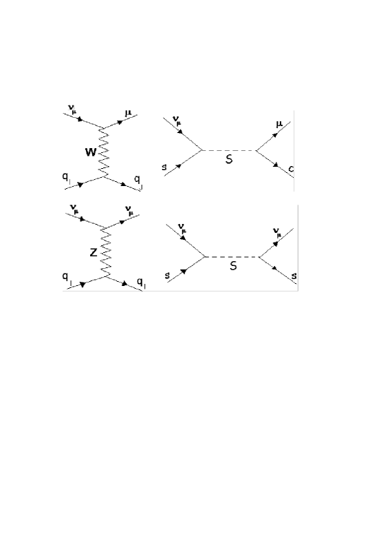
Figure 1: Diagrams contributing to the neutrino-nucleon cross section.

where $Q=(c,s)^{t}$ and $L=(\nu_{\mu},\mu)^{t}$ are the quarks and leptons $SU(2)$ left-handed doublets, $c_{R}$ and $\mu_{R}$ are the right singlets, and $g_{L}$ and $g_{R}$ the corresponding coupling constant.

We are interested in the second family since the directions of the produced muons can be determined with high accuracy.

In figure 1 we show beside the SM contribution for charged and neutral current the leptoquark relevant diagram, where the corresponding cross section for charged and neutral current are given by:

$$\frac{d\sigma^{CC}_{LQ}}{dxdy} = \frac{g_{L}^{2}}{32\pi}(g_{L}^{2}+g_{R}^{2})\frac{\hat{s}}{(\hat{s}-M^{2}_{LQ})^{2}+(\Gamma M_{LQ})^{2}}s(x,M_{LQ})$$

$$\frac{d\sigma^{NC}_{LQ}}{dxdy} = \frac{g_{L}^{4}}{32\pi}\frac{\hat{s}}{(\hat{s}-M^{2}_{LQ})^{2}+(\Gamma M_{LQ})^{2}}s(x,M_{LQ})$$ (2)

where $\hat{s}=xS$, $S=2M_{proton}E_{\nu}$ and the Leptoquark width is $\Gamma=(M_{LQ}/16\pi)(2g_{L}^{2}+g_{R}^{2})$. On the other hand the corresponding SM cross section reads for charged current

$$\begin{split}\frac{d\sigma^{CC}}{dxdy}=\frac{G_{F}^{2}s}{\pi}\left(\frac{M_{W}^{2}}{(Q^{2}+M_{W}^{2})}\right)^{2}x[Q^{CC}+(1-y)^{2}\bar{Q}^{CC}],\end{split}$$ (3)

and for the neutral current

$$\begin{split}\frac{d\sigma^{NC}}{dxdy}=\frac{G_{F}^{2}s}{\pi}\left(\frac{M_{Z}^{2}}{Q^{2}+M_{Z}^{2}}\right)^{2}\sum_{i=U,D}x[g^{i2}_{L}(Q^{i}+(1-y)^{2}\bar{Q}^{i})\\ +g^{i2}_{R}(\bar{Q}^{i}+(1-y)^{2}Q^{i})],\end{split}$$ (4)

where the quark combinations $\bar{Q}^{CC}$, $Q^{CC}$, $\bar{Q}^{i}$ and $Q^{i}$ for a isoscalar target are given in alfa ; gandhi and $g^{U}_{L}=1/2-2x_{W}/3$, $g^{D}_{L}=-1/2+x_{W}/3$, $g^{U}_{R}=-2x_{W}/3$, $g^{D}_{R}=x_{W}/3$, $c_{W}=\cos\theta_{W}$, $x_{W}=\sin^{2}\theta_{W}$.

In Fig. 2 we show the behavior of the total cross section ($\sigma^{t}(E)=\sigma^{CC}(E)+\sigma^{NC}(E)$) with the neutrino energy for different values of $M_{LQ}$ and the couplings $g_{L}=g_{R}=1$. We can appreciate a disagreement with the SM predictions, due to the leptoquark contribution for values of $E_{\nu}$ where the leptoquark can be on shell.

Figure 2: Total cross section for the SM and for different values of the leptoquark mass $M_{LQ}$ and for $g_{L}=g_{R}=1$.

II The surviving neutrino flux

The surviving flux of neutrinos of energy $E$, with inclination $\theta$ with respect to nadir direction, $\Phi(E,\theta)$, is the solution of the complete transport equation nicolaidis :

$$\frac{d\ln\Phi(E,\tau^{\prime})}{d\tau^{\prime}}=-\sigma^{t}(E)+\int_{E}^{\infty}dE^{\prime}\frac{\Phi(E^{\prime},\tau^{\prime})}{\Phi(E,\tau^{\prime})}\;\frac{d\sigma^{NC}}{dE},$$ (5)

where the first term correspond to absorption effects and the second one to the regeneration. Here, $0<\tau^{{}^{\prime}}<\tau(\theta)$ where $\tau=\tau(\theta)$ is the number of nucleons per unit area in the neutrino path through the Earth,

$$\tau(\theta)=N_{A}\int_{0}^{2R_{\rm E}\cos\theta}\rho(z)dz,$$ (6)

$N_{A}$ is the Avogradro number, $R_{\rm E}$ is the radius of the Earth, $\theta$ is the nadir angle taken from the down-going normal to the neutrino telescope and the earth density $\rho(r)$ is given by the preliminary reference earth model premm . In order to find a solution for this equation we make the following approximation ralston : we replace the fluxes ratio inside the integral of the second member by the ratio of fluxes that solve the homogeneous equation (i.e., only considering absorption effects)

$$\frac{\Phi(E^{\prime},\tau^{\prime})}{\Phi(E,\tau^{\prime})}\;\;\rightarrow\;\;\frac{\Phi_{0}(E^{\prime},\theta)}{\Phi_{0}(E,\theta)}e^{-\Delta(E^{\prime},E)\tau^{\prime}}$$ (7)

where $\Delta(E^{\prime},E)=[\;\sigma^{t}(E^{\prime})-\sigma^{t}(E)\;]$ and $\Phi_{0}(E^{\prime},\theta)$ is the initial flux at the earth surface. How we explain later, we will use the initial flow given by the sum of the atmospheric flux, with a well-known angular dependency, with a diffuse and isotropic cosmic flux. Thus, integrating the transport equation we have

$$\Phi(E,\theta)=\Phi_{0}(E,\theta)e^{-\sigma_{eff}(E,\theta)\tau(\theta)},$$ (8)

where

$$\sigma_{eff}(E,\theta)=\sigma^{t}(E)-\sigma^{reg}(E,\theta),$$ (9)

with

$$\sigma^{reg}(E,\theta)=\int_{E}^{\infty}dE^{\prime}\;\frac{d\sigma^{NC}}{dE}\left(\frac{\Phi_{0}(E^{\prime},\theta)}{\Phi_{0}(E,\theta)}\right)\left(\frac{1-e^{-\Delta(E^{\prime},E)\tau(\theta)}}{\tau(\theta)\Delta(E^{\prime},E)}\right).$$ (10)

It is important to mention that the solution of the transport equation, Eq. (8) is the first, but quite accurate, approximation of the iterative method showed in Ref.perrone .

III The Observable $\alpha(E)$

A kilometer cubic neutrino telescope as IceCube is capable of probing fundamental questions of ultra-high energy neutrino interactions. Disagreement with the Standard Model prediction for the cross section could be an indication of new physics. The problem is that the knowledge of neutrino flux and neutrino-nucleon cross section must be built up simultaneously, since we are largely ignorant of both in the energy regime of interest. The knowledge of one is dependent on knowledge of the other. In these conditions we have defined in a previous work alfa an observable ($\alpha(E)$) to search effects of new physic in the neutrino-nucleon interaction. This new observable works by comparing the surviving flux at the detector such that the observable is weakly dependent of the initial flux.

Figure 3: The utilized flux obtained by adding the atmospheric and the isotropical cosmic flux.

The angle $\alpha(E)$ and the related ratio $\eta(E)$ introduced in Ref.alfa are the observable that we shall use in this paper in order to study the impact of leptoquark physics on neutrino detection in a neutrino telescope such as IceCube. By definition $\alpha(E)$ is the angle that divides the Earth into two homo-event sectors. When neutrinos traverse the planet in their journey to the detector, they find different matter densities, and then, different number of nucleons to interact with. In this conditions, the number of neutrinos that finally arrive to the detector depends on the arrival directions, indicated by the angle $\theta$ with respect to the nadir direction. If we consider only upward-going neutrinos of a given energy $E$, that is, the ones with arrival directions $\theta$ such that $0<\theta<\pi/2$, there will always exist an angle $\alpha(E)$ such that the number of events for $0<\theta<\alpha(E)$ equals that for $\alpha(E)<\theta<\pi/2$.

Clearly, the value of $\alpha(E)$ is energy dependent. For low energies, the cross section decreases and the Earth becomes transparent to neutrinos. In this case $\alpha(E)\rightarrow\pi/3$ for a diffuse isotropic flux since this angle divides the hemisphere into two sectors with the same solid angle. Obviously for extremely high energies, where most neutrinos are absorbed, $\alpha(E)\rightarrow\pi/2$, and for intermediate energies $\alpha(E)$ varies accordingly between these limiting behaviors.

In order to define $\alpha(E)$ we consider the expected number of events (muon tracks though charged currents $\nu_{\mu}N$ interactions) at IceCube in the energy interval $\Delta E$ and in the angular interval $\Delta\theta$ that can be estimated as

$${\mathcal{N}}=n_{\rm T}T\int_{\Delta\theta}\int_{\Delta E}d\Omega dE_{\nu}\sigma^{CC}(E)\Phi(E,\theta),$$ (11)

where $n_{\rm T}$ is the number of target nucleons in the effective detection volume, $T$ is the running time, and $\sigma^{CC}(E)$ is the charged neutrino-nucleon cross section. We take the detection volume for the events equal to the instrumented volume for IceCube, which is roughly 1 km³ and corresponds to $n_{\rm T}\simeq 6\times 10^{38}$. The function $\Phi(E,\theta)$ in Eq.(11) is the survival flux which is the solution (Eq.(8)) of the complete transport equation nicolaidis .

The definition of $\alpha(E)$ is essentially the equality between two number of events, thus, to a good approximation, for each energy bin all the previous factors cancel except the integrated fluxes at each side. In this way, $\alpha(E)$ can be defined by the equation

$$\int_{0}^{\alpha(E)}d\theta\sin\theta\;\Phi_{0}(E,\theta)e^{-\sigma_{eff}(E,\theta)\tau(\theta)}=\int_{\alpha(E)}^{\pi/2}d\theta\sin\theta\;\Phi_{0}(E,\theta)e^{-\sigma_{eff}(E,\theta)\tau(\theta)},$$ (12)

which is numerically solved to give the results shown in the Fig. 4(solid line). There we show the SM prediction for $\alpha(E)$, the theoretical uncertainties as we explain below and the leptoquarks contribution for different values of the mass $M_{LQ}$ and for the coupling $g=g_{L}=g_{R}=1$.

Figure 4: The predictions for $\alpha(E)$ obtained for different values of $M_{LQ}$. The shaded region represent the theoretical uncertainties for $\alpha_{SM}(E)$.

The main characteristics of $\alpha(E)$ have been reported recently in Ref.alfa . It is worth to notice that $\alpha(E)$ is weakly dependent on the initial flux but, at the same time it is strongly dependent on the neutrino nucleon cross-section. Hence, the use of the observable $\alpha(E)$ reduces the effects of the experimental systematics and initial flux dependence. Since the functional form of $\alpha(E)$ sharply depends on the interaction cross section neutrino-nucleon, if physics beyond the SM operates at these high energies it will become manifest directly onto the function $\alpha(E)$.

In order to evaluate the impact of the observable $\alpha(E)$ to bound new physics effects, we have estimated the corresponding uncertainties on the SM prediction for $\alpha(E)$. Considering the number of events as distributed according to a Poisson distribution the uncertainty can be propagated onto the angle $\alpha_{\rm SM}(E)$. The number of events $N$ as a function of $\alpha_{\rm SM}$ is

$$N=2\pi n_{\rm T}T\Delta E\sigma^{CC}(E)\int_{0}^{\alpha_{\rm SM}}d\theta\sin\theta\;\Phi_{0}(E,\theta)e^{-\sigma_{eff}(E,\theta)\tau(\theta)},$$ (13)

where we have considered the effective volume for contained events so that an accurate and simultaneous determination of the muon energy and shower energy is possible and then of the neutrino energy. For IceCube, it corresponds to the instrumented volume, roughly 1 km³, implying a number of target nucleons $n_{\rm T}\simeq 6\times 10^{38}$. We have considered an integration time $T=15$ yr which is the expected lifetime of the experiment. To propagate the error on $N$ to obtain the one on $\alpha$, we note that

$$\delta N=\dfrac{dN}{d\alpha}\delta\alpha,$$ (14)

and dividing by $N$ we obtain the statistical errors on $\alpha$

$$\delta\alpha=\left[\int^{\alpha_{\rm SM}(E)}_{0}d\theta\left(\dfrac{\sin\theta}{\sin\alpha_{\rm SM}}\right)\left(\dfrac{\Phi_{0}(E,\theta)}{\Phi_{0}(E,\alpha_{SM})}\right)\dfrac{\exp{[-\sigma_{eff}(E,\theta)\tau(\theta)]}}{\exp{[-\sigma_{eff}(E,\alpha_{SM})\tau(\alpha_{SM})]}}\right]\left(\dfrac{\delta N}{N}\right),$$ (15)

where for Poisson distributed events we have

$$\delta N=\sqrt{N}.$$ (16)

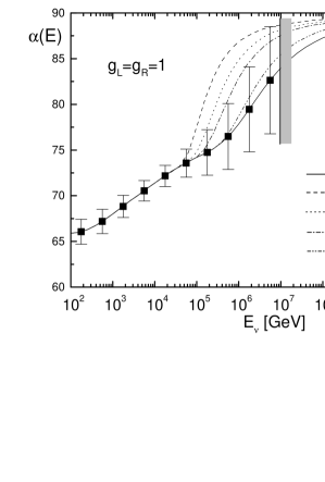
Figure 5: The predictions for $\alpha(E)$ obtained for different values of $M_{LQ}$. The indicated errors are obtained by adding in quadrature the theoretical uncertainties and the statistical errors as it just was explained in the text.

In order to evaluate the errors on $\alpha(E)$, it is necessary to consider a level of initial flux $\Phi_{0}(E,\theta)$. Here we have added together the cosmological diffuse isotropic flux and the atmospheric one(see Fig. 3). For the atmospheric flux, we have considered the one given in Ref.atmos . For the cosmological diffuse flux, the usual benchmark is the so-called Waxman-Bahcall (WB) flux for each flavor, $E_{\nu_{\mu}}^{2}\phi_{\rm WB}^{\nu_{\mu}}\simeq 2.4\times 10^{-8}{\rm GeV}\ {\rm cm}^{-2}{\rm s}^{-1}{\rm sr}^{-1}$, which is derived assuming that neutrinos come from transparent cosmic ray sources waxman-bahcall , and that there is an adequate transfer of energy to pions following $pp$ collisions. However, one should keep in mind that if there are in fact hidden sources which are opaque to ultra-high energy cosmic rays, then the expected neutrino flux will be higher.

On the other hand, we have the experimental bounds set by AMANDA. A summary of these bounds can be found in Refs.desiati ; amanda-bound and as a representative value we take $E_{\nu_{\mu}}^{2}\phi_{\rm AM}^{\nu_{\mu}}\simeq 8\times 10^{-8}{\rm GeV}\ {\rm cm}^{-2}{\rm s}^{-1}{\rm sr}^{-1}$. With the intention to estimate the number of events, we have considered an intermediate flux (INT) level slightly below the present experimental bound by AMANDA,

$$E_{\nu_{\mu}}^{2}\phi_{\rm INT}^{\nu_{\mu}}\simeq 5\times 10^{-8}{\rm GeV}\ {\rm cm}^{-2}{\rm s}^{-1}{\rm sr}^{-1}.$$ (17)

Moreover we have considered the theoretical uncertainties on the observable $\alpha_{SM}(E)$, which come from the uncertainties in the earth density, the standard model neutrino-nucleon cross section and the initial neutrino flux. As we explained above, we have considered the initial flux as the sum between the atmospheric flux and an isotropic diffuse cosmic flux. The observable $\alpha(E)$ is weakly dependent on the isotropic uncertainties in the cosmic flux, but it is dependent on the anisotropic uncertainties in the atmospheric flux. Uncertainties in the calculated neutrino intensity arise from lack precise knowledge of the input quantities, which are the primary spectrum and the inclusive cross section for production of pions and kaons by hadronic interaction in the atmosphere. If we consider the primary spectrum as isotropic then, the corresponding uncertainties do not affect significatively to $\alpha(E)$. Any isotropic overall factor that we include to modify the initial atmospheric flux do not produce higher effects on $\alpha(E)$ because it is defined by comparing the number of events from different angular directions. In this conditions the principal source of uncertainties is the inclusive cross section for production of pions and kaons. We include theoretical uncertainties in the energy-angular dependence in the atmospheric flux due to the uncertainties in the $K/\pi$ ratio as an angular uncertainty between horizontal and vertical neutrino events. In order to take into account these uncertainties and their effect on $\alpha(E)$ we have multiplied the atmospheric initial flux by an angular dependent factor, imposing opposite uncertainties of $\pm$10% to horizontal and vertical flux respectively and interpolating for intermediate angular values. In a similar way we have taken into account the uncertainties that come from the earth density and the neutrino-nucleon cross section premm ; saakar , such that it maximize the uncertainties on $\alpha(E)$. The results are shown as shaded region in Fig.4.

We consider the theoretical uncertainties discussed above and the statistical errors (Eq.(15)) as uncorrelated statistical errors and we sum them in quadrature. The results are shown as error bars in Fig.(5).

As it was discussed in Ref.alfa the interval for maximum sensitivity for $\alpha$ is $10^{5}\rm{GeV}<E<10^{7}\rm{GeV}$. However, as for lower energies the atmospheric flux grows and then the statistical errors fall, we have considered as an energy window for the fits the interval: $10^{2}\rm{GeV}<E<10^{7}\rm{GeV}$. In Fig. 5 we show our results for the observable $\alpha(E)$ and the corresponding errors within the mentioned energy window. In Fig. 3 we show the used flux.

In the same context, we can define another observable related to $\alpha(E)$. We consider the hemisphere $0<\theta<\pi/2$ divided into two regions by the angle $\alpha_{SM}(E)$, ${\cal R}_{1}$ for $0<\theta<\alpha_{SM}(E)$ and ${\cal R}_{2}$ for $\alpha_{SM}(E)<\theta<\pi/2$. We then calculate the ratio $\eta(E)$ between the number of events for each region,

$$\eta(E)=\frac{N_{1}}{N_{2}},$$ (18)

where $N_{1}$ is the number of events in the region ${\cal R}_{1}$ and $N_{2}$ the number of events in the region ${\cal R}_{2}$. By using $\eta(E)$ the effects of experimental systematic and initial flux dependence are reduced. If there is only SM physics, then we have that the ratio $\eta_{SM}(E)=1$. In order to estimate the capability of $\eta(E)$ to bound leptoquarks effects, we have considered the values of $\eta(E)$ along with their error bars in Fig. 7 as if they had been obtained from experimental measurements for $\eta(E)$. We proceed, then, to perform a $\chi^{2}$-analysis taking as free parameters the leptoquark mass $M_{LQ}$ and the couplings $g=g_{L}=g_{R}$ and considering as experimental point the SM values for $\eta(E)$ for the same energy bin used in Fig. 5. We define the $\chi^{2}$ function in the usual way,

$$\chi^{2}=\sum_{i=1,10}\dfrac{(\eta_{\rm SM}(E_{i})-\eta(E_{i},M_{LQ},g))^{2}}{(\delta\eta(E_{i}))^{2}}.$$ (19)

Figure 6: $\eta(E)$ for different values of $M_{LQ}$. We include the theoretical uncertainties as a shaded region around the standard model value $\eta=1$.

where $\delta\eta$ are errors obtained by adding in quadrature the statistical errors and the theoretical uncertainties. According to the definition of $\eta(E)$ (Eq.(18)) the statistical errors are given by $\delta\eta_{st}(E_{i})=\sqrt{2/N_{i}}$ for events distributed according to a Poisson distribution. In the same way that we have done for $\alpha(E)$ we can propagate the theoretical uncertainties on the observable $\eta(E)$ and these are show in Fig.(6) as a shaded region around the Standard Model prediction ($\eta=1$). These theoretical uncertainties are added in quadrature with the statistical errors for $\eta(E)$ and the results are show as errors bar in the Fig(7). Is important to realize that the atmospheric flux is lower than the cosmic one for energies higher than $10^{5}GeV$. In the other hand the leptoquark contribution is very small for energies lower than $10^{5}GeV$. In this conditions we do not expect a strong dependence of the leptoquarks bounds on the atmospheric flux uncertainties.

The function $\chi^{2}$ is minimized to obtain the allowed region in the ($M_{LQ}$, $g$) plane for $g_{L}=g_{R}=g$, which corresponds to the region below the curve shown in Fig. 8. In the same figure we also include the bounds obtained from the D0 experiment obtained for the second family (vertical line) d0 .

Figure 7: $\eta(E)$ for different values of $M_{LQ}$. We include the statistical errors obtained of a number of events distributed as a Poisson distribution added in quadrature with the theoretical uncertainties as it was explained in the text.

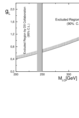
Figure 8: The excluded regions in the $(M_{LQ},g)$ plane (for $g_{L}=g_{R}=g$) is above the curve. The region to left the vertical is excluded by D0 d0 .

IV Conclusions

In the present work we studied the effects of leptoquarks contributions to the neutrino-nucleon cross section on the survival neutrino flux in a neutrino telescope like IceCube. We have found a considerable disagreement with the SM prediction for the neutrino observables defined above, particulary for low values of $M_{LQ}$. For high values of $M_{LQ}$ this disagreement tends to disappear.

We have also studied the possibility to bound effects of leptoquarks contributions to the interactions between muon neutrinos and the nucleons of the Earth using the observable $\eta(E)$. In this context, we fitted the theoretical expression for $\eta(E)$ as a function of the $M_{LQ}$ and $g=g_{L}=g_{R}$ taking as experimental data the SM values obtained for $\eta$ ($\eta_{SM}(E)=1$) along with the errors that come from the theoretical uncertainties and the number of events distributed according to a Poisson distribution. The results are shown in Fig. 8 as a allowed region plot. Finally, would like comment that a similar region was obtained in Ref. leptogarcia , but using the down-going neutrinos and the inelasticity distribution of events as an useful observable also defined in IceCube. Perhaps, the simultaneous use of both methods will make possible to improve the bounds on leptoquarks physics.

- (1) W. M. Yao et al. Journal of Physics G 33 (2006) 1.
- (2) M.C. Gonzalez-Garcia. Phys. Lett. B663 (2008) 405.
- (3) M. M. Reynoso and O. A. Sampayo, Phys.Rev.D76 (2007) 033003.
- (4) O.A.Sampayo and M.Reynoso, Acta Phys. Pol. 39 (2008) 599, I.Romero and O.A.Sampayo Mod. Phys. Lett. A24 (2009) 523, G.Gonzalez-Sprimberg, R.Martinez and O.A.Sampayo Phys. Rev. D79 (2009) 053005.
- (5) L.A.Anchordoqui, C.A.Garcia Canal, H.Goldberg, D.Gomez Dumm and F.Halzen, Phys. Rev. D74 (2006) 125021.
- (6) L.Anchordoqui, M.Glenz and L.Parker, Phys.Rev.D75 (2007) 024011.
- (7) W.Buchmuller, R.Ruckl and Wyler, Phys.Lett.B 191 (1987) 442 [Erratum-ibid. B 448, 320 (199)].
- (8) H.Georgi and S.L.Glashow, Phys. Rev. Lett. 32, (1974) 438. J.C.Pati and A.Salam, Phys. Rev. D 10 (1974) 275.
- (9) A.Y.Smirnov and F.Vissani, Phys. Lett. B 380 (1996) 317.
- (10) R. Gandhi, C. Quigg, M. H. Reno, I. Sarcevic, Astropart. Phys. 5 (1996) 81.
- (11) A. Nicolaidis and A. Taramopoulus, Phys. Lett. B 386 (1996) 211.
- (12) A. M. Dziewonski and D. L. Anderson, Phys. Earth Planet Inter. 25 (1981) 297.
- (13) P. Jain, S. Kar, D. W. McKay, S. Panda, J. P. Ralston, Phys. ReV. D 66 (2002) 065018.
- (14) V.A.Naumov and L.Perrone., Astropart. Phys. 10 (1999) 239.
- (15) V.Agrawal, T.K.Gaisser, P.Lipari and T.Stanev, Physical Review D 53 (1996) 1314.
- (16) E. Waxman and J. N. Bahcall, Phys. Rev. D 59 (1999) 023002.
- (17) P. Desiati, [astro-ph/0611603]
- (18) M. Ackermann et al, Astropart. Phys. 22 (2005) 339.
- (19) A.Cooper-Sarkar and S.Sarkar, JHEP0801 (2008) 075.
- (20) V.M.Abazov et al. [D0 collaboration], Phys. Lett. B636 (2006) 183. [hep-ph/0601047].