Quantum Interference Effects in Spacetime of Slowly Rotating Compact Objects in Braneworld

Mamadjanov A.I., Hakimov A.A., Tojiev S.R.

Abstract

The phase shift a neutron interferometer caused by the gravitational field and the rotation of the earth is derived in a unified way from the standpoint of general relativity. General relativistic quantum interference effects in the slowly rotating braneworld as the Sagnac effect and phase shift effect of interfering particle in neutron interferometer are considered. It was found that in the case of the Sagnac effect the influence of brane parameter is becoming important due to the fact that the angular velocity of the locally non rotating observer must be larger than one in the Kerr space-time. In the case of neutron interferometry it is found that due to the presence of the parameter $Q^{*}$ an additional term in the phase shift of interfering particle emerges from the results of the recent experiments we have obtained upper limit for the tidal charge as $Q^{*}\lesssim 10^{7}\rm{cm}^{2}$. Finally, as an example, we apply the obtained results to the calculation of the (ultra-cold neutrons) energy level modification in the braneworld.

1 Introduction

The detection of gravitational radiation provides not only a verification of the predictions of general relativity, but also opens a new window for astronomical observations. In this respect, it is desirable to understand thoroughly the general relativistic effects on the quantum mechanical interference. It would be of great significance to have a formalism to derive these various effects in a unified way. The aim of this paper is to show such a treatment. We show that the Sagnac effect and phase shift effect in a neutron interferometer in the braneworld.

The idea that our Universe might be a three-brane [1], emdedded in a higher dimensional spacetime, has recently attracted much attention. Static and spherically symmetric exterior vacuum solutions of the brane world models were initially proposed by Dadhich et al [2, 3] which have the mathematical form of the Reissner-Nordström solution, in which a tidal Weyl parameter $Q^{*}$ plays the role of the electric charge of the general relativistic solution. The role of the tidal charge in the orbital resonance model of quasiperiodic oscillations in black hole systems [4] and in neutron star binary systems [5] have been studied intensively. The so-called DMPR solution was obtained by imposing the null energy condition on the three-brane for a bulk having nonzero Weyl curvature. In this paper we testing the Sagnac effect and phase shift effect in a neutron interferometer in that the braneworld.

The experiment to test the effect of the gravitational field of the Earth on the phase shift in a neutron interferometer were first proposed by Overhauser and Colella [6]. Then this experiment was successfully performed by Collela, Overhauser and Werner [7]. After that, there were found other effects, related with the phase shift of interfering particles. Among them the effect due to the rotation of the Earth [8, 9], which is the quantum mechanical analog of the Sagnac effect, and the Lense-Thirring effect [10] which is a general relativistic effect due to the dragging of the reference frames. So we do not consider the neutron spin in this paper

In the paper [11] a unified way of study of the effects of phase shift in neutron interferometer due to the various phenomena was proposed. Here we extend this formalism to the case of the slowly rotating braneworld in order to derive such phase shift due to either existence or nonexistence of the tidal brane charge.

The Sagnac effect is well known and thoroughly studied in the paper [12]. It presents the fact that between light or matter beam counter-propagating along a closed path in a rotating interferometer a fringe shift $\triangle\varphi$ arises. This phase shift can be interpreted as a time delay $\triangle T$ between two beams, as it can be seen below, doesn’t include the mass or energy of particles. That is why we may consider the Sagnac effect as the ”universal” effect of the geometry of space-time, independent of the physical nature of the interfering beams. Here we extend the recent results obtained in the papers [13, 14] where it has been shown a way of calculation of this effect in analogy with the Aharonov-Bohm effect, to the case of slowly rotating braneworld.

The paper is organized as follows. In section 2, we taking starting from the covariant. Klein-Gordon equation in the braneworld , and consider terms the phase difference of the wave function. In section 3 we consider interference in Mach-Zender interferometer in the background of spacetime of black hole in braneworld. Section 4 is devoted to study Sagnac effect in the slowly rotating braneworld.

Recently Granit experiment [15] verified the quantization of the energy level of ultra-cold neutrons (UCN) in the Earth’s gravity field and new, more precise experiments are planned to be performed. Experiments with UCN have high accuracy and that is the reason to look for verification of the gravitomagnetism in such experiments. As an example we investigate modification of UCN energy levels caused by the existence of brane parameter.

Throughout, we use space-like signature ( -, +, +, +) (However, for those expressions with an astrophysical application we have written the speed of light explicitly). Greek indices are taken to run from 0 to 3 and Latin indices from 1 to 3; covariant derivatives are denoted with a semi-colon and partial derivatives with a comma.

2 The Phase shift

We assume that the external gravitational field of the earth is described by the braneworld model proposed recently in papers [11]. Slowly rotating gravitating object in braneworld in a spherical coordinate system is described by the metric .

$$ds^{2}=-A^{2}dt^{2}+H^{2}dr^{2}+r^{2}d\theta^{2}+r^{2}\sin^{2}\theta d\phi^{2}-2\widetilde{\omega}(r)r^{2}\sin^{2}\theta dtd\phi,$$ (1)

here

$$A^{2}(r)\equiv\left(1-\frac{2M}{r}+\frac{Q^{*}}{r^{2}}\right)=H^{-2},$$ (2)

is the Reissner-Nordström-type exact solution [2] for the metric outside the gravitating object and $\widetilde{\omega}(r)=\omega(1-\frac{Q^{*}}{2rM})=2Ma/r^{3}(1-Q^{*}/2rM)$.

Using the Klein-Gordon equation

$$\nabla^{\mu}\nabla_{\mu}\Phi-(mc/\hbar)^{2}\Phi=0,$$ (3)

for particles which have a mass $m$, in the paper [11] it was defined the wave function $\Phi$ of interfering particles as

$$\Phi=\Psi exp\left(-i\frac{mc^{2}}{\hbar}t\right)\ ,$$ (4)

where $\Psi$ is the nonrelativistic wave function.

In the present situation, both $GM/rc^{2}$ and $a/r$ are sufficiently small and their higher order terms can be neglected. Therefore, to the first order in $M$ and $Q$ and neglecting the terms of $O((\upsilon/c)^{2})$, the Klein-Gordon equation in the braneworld becomes

$$i\hbar\frac{\partial\Psi}{\partial t}=-\frac{\hbar^{2}}{2m}\left[\frac{1}{r^{2}}\frac{\partial}{\partial r}\left(r^{2}\frac{\partial}{\partial r}\right)-\frac{L^{2}}{r^{2}\hbar^{2}}\right]\Psi-\frac{GMm}{r}\Psi+\frac{Q^{*}mc^{2}}{2r^{2}}\Psi+\frac{2GMa}{r^{3}c}(1-\frac{Q^{*}}{r^{2}}-\frac{Q^{*}c^{2}}{2rMG})L_{z}\Psi\ ,$$ (5)

where we have used the following notations:

$$L^{2}=-\hbar^{2}\left[\frac{1}{\sin\theta}\frac{\partial}{\partial\theta}\left(\sin\theta\frac{\partial}{\partial\theta}\right)+\frac{1}{\sin^{2}\theta}\frac{\partial^{2}}{\partial\phi^{2}}\right]\ ,$$ (6)

$$L_{z}=-i\hbar\frac{\partial}{\partial\phi}\ ,$$ (7)

which correspond the square of the total orbital angular momentum and $z$ component of the orbital angular momentum operators of the particle with respect to the center of the earth, respectively. After the coordinate transformation $\phi\rightarrow\phi+\Omega t$, where $\Omega$ is the angular velocity of the earth, we obtain the Schrödinger equation for an observer fixed on the earth in the following form:

$$i\hbar\frac{\partial\Psi}{\partial t}=-\frac{\hbar^{2}}{2m}\left[\frac{1}{r^{2}}\frac{\partial}{\partial r}\left(r^{2}\frac{\partial}{\partial r}\right)-\frac{L^{2}}{r^{2}\hbar^{2}}\right]\Psi-\frac{GMm}{r}\Psi+\frac{Q^{*}mc^{2}}{2r^{2}}\Psi-\Omega L_{z}\Psi$$

$$\qquad\qquad+\frac{2GMa}{r^{3}c}L_{z}\Psi-\frac{GQ^{*}ac}{r^{4}}\left(1+\frac{2GM}{c^{2}r}\right)L_{z}\Psi\ .$$ (8)

The Hamiltonian derived in the last section can be divided in to the five terms as:

$$H=H_{0}+H_{1}+H_{2}+H_{3}+H_{4},$$ (9)

where

$$H_{0}=-\frac{\hbar^{2}}{2m}\frac{1}{r^{2}}\frac{\partial}{\partial r}\left(r^{2}\frac{\partial}{\partial r}\right)+\frac{L^{2}}{2mr^{2}}\ ,\quad H_{1}=-\frac{GMm}{r}+\frac{Q^{*}mc^{2}}{2r^{2}}\ ,\quad H_{2}=-\Omega L_{z}\ ,\quad$$

$$H_{3}=\frac{2GMa}{r^{3}c}L_{z}\ ,\quad\quad H_{4}=-\frac{Q^{*}ac}{r^{4}}\left(1+\frac{2GM}{c^{2}r}\right)L_{z}.$$ (10)

$H_{0}$ is the Hamiltonian for a freely propagating particle, $H_{1}$ is the Newtonian gravitational potential energy, $H_{2}$ is concerned to the rotation of the gravitating source, $H_{3}$ is related to the Lense-Thirring effect (dragging of the inertial frames). The phase shift terms due to $H_{1},H_{2}$ and $H_{3}$ are

$$\beta_{Sag}\simeq\frac{2m\bf{\Omega}\cdot\textbf{S}}{\hbar}\ ,\quad\beta_{drag}\simeq\frac{2Gm}{\hbar c^{2}R^{3}}\textbf{J}\cdot\left[\textbf{S}-3\left(\frac{\textbf{R}}{R}\cdot\textbf{S}\right)\frac{\textbf{R}}{R}\right]\ ,$$ (11)

respectively and in the first place, let us calculate the phase shift due to the gravitational potential. For the purpose of the present discussion, the quasi-classical approximation is valid and the phase shift is given by the integration along a classical trajectory (see.fig 1)

$$\beta_{grav}=\beta_{ABD}-\beta_{ACD}=-\frac{1}{\hbar}\int\frac{GQ^{*}a}{r^{4}}\left(1+\frac{2M}{r}\right)dr\simeq\frac{m^{2}S\lambda}{2\pi\hbar^{2}}\left(g-\frac{Q^{*}c^{2}}{R^{3}}\right)\sin\phi\ \ .$$ (12)

The phase difference $\beta_{grav}$ will be

$$\beta_{grav}=\left[\frac{m^{2}S\lambda g}{2\pi\hbar^{2}}-\frac{m^{2}S\lambda}{2\pi\hbar^{2}}\cdot\frac{Q^{*}c^{2}}{R^{3}}\right]=\beta\pm\Delta\beta\ .$$ (13)

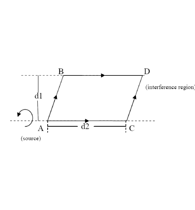
Figure 1: Schematic illustration of alternate paths separated in vertical direction in a neutron interferometer.

As we know according to the experiment [7] the phase difference due to the gravitational potential of the earth was in good agreement with the theoretical prediction within an error of $1\%$. Therefore one can easily obtain the following upper limit for the module of the tidal brane charge as:

$$Q^{*}\lesssim 10^{7}\rm{sm}^{2}\ .$$ (14)

Here $S=d_{1}d_{2}$ is the area of interferometer, $\bf S$ is the area vector of the sector ABCD (see fig. 1), ${\bf\Omega}=(0,0,\Omega)$ and ${\bf J}=(0,0,J)$ are the angular velocity and the angular momentum vectors of the object correspondingly, $\bf R$ is the position vector of the instrument from the center of the gravitating object, $\lambda$ is de Broglie wavelength.

The last term of the equation (10) represents the parts $H_{4}$ Hamiltonian

$$H_{4}=-\frac{Q^{*}ac}{r^{4}}\left(1+\frac{2GM}{c^{2}r}\right)L_{z}\ ,$$ (15)

related to the $Q^{*}$-Brane parameter.

Integrating it over time along the trajectory of the particle, one can find the corresponding phase shift

$$\beta_{4}=-\frac{1}{\hbar}\int\frac{2GMQ^{*}a}{r^{5}c}L_{z}dt,\quad\beta_{5}=-\frac{1}{\hbar}\int\frac{Q^{*}ac}{r^{4}}L_{z}dt\ .$$ (16)

Presenting ${\bf r}={\bf R}+{\bf r^{\prime}}$, where $\bf r^{\prime}$ denotes position of the given point of the interferometer from the center of the instrument, and assuming that $r^{\prime}/R$ is small one can obtain that the angular dependence of $\beta_{brane}$

$$\beta_{brane}=\beta_{4(ABD)}-\beta_{4(ACD)}=\frac{2GQ^{*}m}{\hbar c^{2}}\oint\frac{{\bf J}\cdot({\bf r}\times d{\bf r})}{r^{5}}=\frac{2GQ^{*}m}{\hbar c^{2}}{\bf J}\cdot\oint\frac{({\bf R}+{\bf r^{\prime}})\times d{\bf r^{\prime}}}{|{{\bf R}}+{\bf r^{\prime}}|^{5}}$$

$$\simeq-\frac{2GQ^{*}m}{\hbar c^{2}R^{5}}{{\bf J}}\cdot\left[\oint{\bf r^{\prime}}\times d{\bf r^{\prime}}-5\oint\left(\frac{{\bf R}}{R}\cdot\textbf{r}^{\prime}\right)\frac{{{\bf R}}}{R}\times d\textbf{r}^{\prime}\right]=-\frac{2GQ^{*}m}{\hbar c^{2}R^{5}}{{\bf J}}\left[\textbf{S}-5\left(\frac{{\bf R}}{R}\cdot\textbf{S}\right)\frac{{\bf R}}{R}\right]\ ,$$ (17)

and

$$\beta^{\prime}_{brane}=\beta_{5(ABD)}-\beta_{5(ACD)}=\frac{Q^{*}m}{\hbar M}\oint\frac{{\bf J}\cdot(\textbf{r}\times d\textbf{r})}{r^{4}}=\frac{Q^{*}m}{\hbar M}{\bf J}\cdot\oint\frac{({\bf R}+\textbf{r}^{\prime})\times d\textbf{r}^{\prime}}{|{\bf R}+\textbf{r}^{\prime}|^{4}}$$

$$\simeq-\frac{Q^{*}m}{\hbar MR^{4}}{\bf J}\cdot\left[\oint\textbf{r}^{\prime}\times d\textbf{r}^{\prime}-4\oint\left(\frac{{\bf R}}{R}\cdot\textbf{r}^{\prime}\right)\frac{{\bf R}}{R}\times d\textbf{r}^{\prime}\right]=-\frac{Q^{*}m}{\hbar MR^{4}}{\bf J}\left[\textbf{S}-4\left(\frac{{\bf R}}{R}\cdot\textbf{S}\right)\frac{{\bf R}}{R}\right]\ ,$$ (18)

where ${\bf R}$ represents the position vector of the instrument from the center of the earth. If we assume that the earth is a sphere of radius $R$ with uniform density, then

$${\bf J}=\frac{2}{5}MR^{2}{\bf\Omega}\ ,$$ (19)

and, if R is perpendicular to $\bf S$

$$\beta_{brane}=-\frac{1}{5}\frac{r_{g}Q^{*}}{R^{3}}\beta_{Sag},\quad\beta^{\prime}_{brane}=-\frac{1}{5}\frac{Q^{*}}{R^{2}}\beta_{Sag}\ ,$$ (20)

if R is parallel to $\bf S$

$$\beta_{brane}=\frac{4}{5}\frac{r_{g}Q^{*}}{R^{3}}\beta_{Sag},\quad\beta^{\prime}_{brane}=\frac{3}{5}\frac{Q^{*}}{R^{2}}\beta_{Sag}\ ,$$ (21)

where $r_{g}=2GM/c^{2}$ is the Schwarzchild radius of earth.

Astrophysically it is interesting to apply the obtained result for the Hamiltonian of the particle, moving around rotating gravitating object in braneworld, to the calculation of energy level of ultra-cold neutrons (UCN) (as it was done for slowly rotating Kerr space-time in the work [16] and for slowly rotating object with nonvanishing gravitomagnetic charge in the work [17]). Recently it was investigated the effect of the angular momentum perturbation of the Hamiltonian $H_{2}=\Omega L_{z}$ on the energy levels of UCN [16]. Our purpose is generalize this correction to the case of the gravitating object (Earth in particular case) which possess also brane parameter. Denote as the unperturbed non-relativistic stationary state of the 2- spinor (describing UCN) in the field of the rotating gravitating object in braneworld. Then we have

$$H_{4}\psi=i\hbar\frac{Q^{*}ac}{r^{4}}\left(1+\frac{2GM}{c^{2}r}\right)\frac{\partial\psi}{\partial\phi}=i\hbar\frac{Q^{*}ac\sin\theta}{r^{3}}\left(1+\frac{2GM}{c^{2}r}\right)\nabla\psi\cdot e_{\phi}\ ,$$ (22)

here $\nabla\psi$ is the Laplasian of the spherical coordinates, which is usually written as:

$$\nabla\psi=\frac{\partial\psi}{\partial r}e_{r}+\frac{1}{r}\frac{\partial\psi}{\partial\theta}e_{\theta}+\frac{1}{r\sin\theta}\frac{\partial\psi}{\partial\phi}e_{\phi}\ .$$ (23)

By adopting new Catesian coordinates $x,y,z$ within $e_{x}\equiv e_{\phi}$ and axis $z$ being local vertical, when the stationary state is assumed to have the form

$$\phi(x)=\phi_{\upsilon}(z)e^{i(k_{1}x+k_{2}y)}\ ,$$ (24)

one can easily derive from (22)

$$H_{4}\psi=i\hbar\frac{Q^{*}ac\sin\theta}{r^{3}}\left(1+\frac{2GM}{c^{2}r}\right)\frac{\partial\psi}{\partial x}=-\hbar k_{1}\frac{Q^{*}ac\sin\theta}{r^{3}}\left(1+\frac{2GM}{c^{2}r}\right)\psi$$

$$\qquad\qquad=-mu_{1}\frac{Q^{*}ac\sin\theta}{r^{3}}\left(1+\frac{2GM}{c^{2}r}\right)\psi\ ,$$ (25)

where the following notation has been used

$$u_{1}\equiv{\bf u}\cdot\mathbf{e}_{\phi},\quad{\bf u}\equiv\frac{\hbar}{m}(k_{1}\mathbf{e}_{x}+k_{2}\mathbf{e}_{y})\ .$$ (26)

Following to the works [16] and [17] we can compute modification of the energy level as first-order perturbation:

$$(\delta E)_{brane}\simeq\langle\psi|H_{4}\psi\rangle=-mu_{1}\int\frac{Q^{*}ac\sin\theta}{r^{3}}\left(1+\frac{2GM}{c^{2}r}\right)|\psi|^{2}dV\ .$$ (27)

Assume $r=(R+z)\cos\chi$ (where $\chi$ is the latitude angle) and $\sin\theta$ to be equal to 1, that is $\theta=\pi/2$. Assuming now $z\ll{R}$ one can extend (27) as

$$(\delta E^{\prime})_{brane}\simeq\langle\psi|H_{4}\psi\rangle=-mu_{1}\frac{Q^{*}ac}{{R}^{3}\cos^{3}\chi}+mu_{1}\frac{3Q^{*}ac}{{R}^{4}\cos^{3}\chi}\int z|\psi|^{2}dV\ ,$$ (28)

and

$$(\delta E^{\prime\prime})_{brane}\simeq\langle\psi|H_{4}\psi\rangle=-mu_{1}\frac{2GMQ^{*}a}{{R}^{4}c\cos^{4}\chi}+mu_{1}\frac{8GMQ^{*}a}{{R}^{5}c\cos^{4}\chi}\int z|\psi|^{2}dV\ ,$$ (29)

where we have separated equation (27) into two parts as $(\delta E)_{brane}=(\delta E^{\prime})_{brane}+(\delta E^{\prime\prime})_{brane}$. Then we remember that $\int z|\psi|^{2}dV$ is the average value $\langle z\rangle_{n}$ of $z$ for the stationary state $\psi=\psi_{n}$. For further calculation we need to use formulae for $\langle z\rangle_{n}$ from [16]

$$\langle z\rangle_{n}=\frac{2}{3}\frac{E_{n}}{mg}\ .$$ (30)

Now one can easily estimate the relative modification of the energy level $E_{n}$ of the neutrons, placed in braneworld.

$$\frac{(\delta E^{\prime})_{brane}}{E_{n}}\simeq\frac{2u_{1}Q^{*}ac}{R^{4}g\cos^{3}\chi}\ ,\quad\quad\frac{(\delta E^{\prime\prime})_{brane}}{E_{n}}\simeq\frac{16}{3}\frac{GMQ^{*}u_{1}a}{R^{5}g\cos^{4}\chi}=\frac{16}{3}\frac{Q^{*}u_{1}a}{R^{3}\cos^{4}\chi}\ .$$ (31)

We numerically estimate the obtained modification using the following parameters for the Earth: $u_{1}\simeq+10m/s$, $Q\sim 10^{9}sm$, $\cos\chi\simeq 0.71$, $a\simeq 3.97m$, $g\simeq 10m/s^{2}$ and $R\simeq 6.4\cdot 10^{8}sm$, $c\simeq 3\cdot 10^{8}m/s$

$$\frac{(\delta E^{\prime})_{brane}}{E_{n}}\simeq 4\times 10^{-11}\ .$$ (32)

For the surface of the Earth we can neglect $(\delta E^{\prime\prime})_{brane}$ term. From the obtained result (32) one can see, that the in influence of brane parameter will be stronger in the vicinity of compact gravitating objects with small $R$.

3 The interference in a Mach-Zehnder-type interferometer

Spacetime metric of the rotating black hole in braneworld in coordinates ${t,r,\theta,\varphi}$ takes form (see e.g, [18])

$$ds^{2}=-\frac{\Delta-a^{2}\sin^{2}\theta}{\Sigma}dt^{2}+\frac{(\Sigma+a^{2}\sin^{2}\theta)^{2}-\Delta a^{2}}{\Sigma}\sin^{2}\theta d\varphi^{2}$$

$$\qquad\quad+\frac{\Sigma}{\Delta}dr^{2}+\Sigma d\theta^{2}-2\frac{\Sigma+a^{2}\sin^{2}\theta-\Delta}{\Sigma}a\sin^{2}\theta d\varphi dt\ ,\ \quad$$ (33)

where $\Sigma=r^{2}+a^{2}\cos^{2}\theta$, $\Delta=r^{2}+a^{2}-2Mr+Q^{*}$, $Q^{*}$ is the bulk tidal charge, $M$ is the total mass and $a$ is related to the angular momentum of the black hole.

The components of the tetrad frame for the stationary observer for metric (33) are

$${\bf e}_{\hat{t}}^{\mu}=\left(1-\frac{2M}{r}+\frac{Q^{*}}{r^{2}}\right)^{-\frac{1}{2}}\left(1,0,0,0\right),\hskip 19.91684pt{\bf e}_{\mu}^{\hat{t}}=-\left(1-\frac{2M}{r}+\frac{Q^{*}}{r^{2}}\right)^{\frac{1}{2}}\left(1,0,0,\frac{2Mr-Q^{*}}{r^{2}}\right)$$ (34)

$${\bf e}_{\hat{r}}^{\mu}=\left(1-\frac{2M}{r}+\frac{Q^{*}}{r^{2}}\right)^{\frac{1}{2}}(0,1,0,0),\hskip 28.45274pt{\bf e}_{\mu}^{\hat{r}}=\left(1-\frac{2M}{r}+\frac{Q^{*}}{r^{2}}\right)^{-\frac{1}{2}}(0,1,0,0)$$ (35)

$${\bf e}_{\hat{\theta}}^{\mu}=\frac{1}{r}\left(0,0,1,0\right),\hskip 105.2751pt{\bf e}_{\mu}^{\hat{\theta}}=r(0,0,1,0)$$ (36)

$${\bf e}_{\hat{\varphi}}^{\mu}=\frac{1}{r\sin\theta}\left(\frac{Q^{*}-{2M}{r}}{r\sqrt{r^{2}-{2M}{r}+{Q^{*}}}},0,0,1\right),{\bf e}_{\mu}^{\hat{\varphi}}=r\sin\theta(0,0,1,1)$$ (37)

and the acceleration of the Killing trajectories [19] is

$$a_{\mu}=\frac{1}{2}\partial_{\mu}\ln(-g_{00})\ ,$$ (38)

and we obtain for nonvanishing component of the acceleration

$$a_{\hat{r}}=\frac{1}{r}\left(\frac{M}{r}-\frac{Q^{*}}{r^{2}}\right)\left(1-\frac{2M}{r}+\frac{Q^{*}}{r^{2}}\right)^{-\frac{1}{2}}\ .$$ (39)

The nonzero components of rotation tensor of the stationary congruence $\chi_{\mu\nu}$ in the slowly rotating braneworld are given by

$$\chi_{\hat{r}\hat{\varphi}}=\frac{a\sin\theta}{r^{2}}\left(1-\frac{2M}{r}+\frac{Q^{*}}{r^{2}}\right)^{-1}\left(\frac{M}{r}-\frac{Q^{*}}{r^{2}}\right)\ ,$$ (40)

$$\chi_{\hat{\theta}\hat{\varphi}}=\frac{a\cos\theta}{r^{2}}\left(1-\frac{2M}{r}+\frac{Q^{*}}{r^{2}}\right)^{-\frac{1}{2}}\left(\frac{Q^{*}}{r^{2}}-\frac{2M}{r}\right)\ .$$ (41)

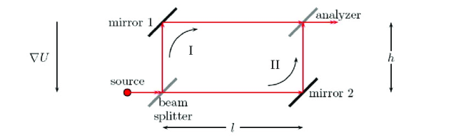
Figure 2: The gradient of $U$ in the interferometer’s rest frame. $h$ and $l$ are the interferometer’s height and length.

Introducing the $\mathcal{A_{\mu}}$ vector potential of the electromagnetic field in the Lorentz gauge in simple form $\mathcal{A}^{\alpha}=C_{1}\xi^{\alpha}_{t}+C_{2}\xi^{\alpha}_{\varphi}$ [20] for the metric (1) with components. There the constant $C_{2}=B/2$, where gravitational source is immersed in the uniform magnetic field $\bf B$ being parallel to its axis of rotation (properties of black hole immersed in external magnetic field have been studied in [21, 22]), and the second constant $C_{1}=aB$ can be calculated from the asymtotic properties of spacetime (1) at the infinity.

$$\mathcal{A}_{t}=-aB\left[1-\left(\frac{2M}{r}-\frac{Q^{*}}{r^{2}}\right)\left(1-\frac{1}{2}\sin^{2}\theta\right)\right]\ ,$$ (42)

$$\mathcal{A}_{\varphi}=\frac{Br^{2}}{2}\sin^{2}\theta\ ,$$ (43)

we can write the total energy of the particle in the weak field approximation in the following form:

$$\mathcal{E}=p(\xi)+\mathcal{E}_{pot}=p(\xi)+e_{p}\mathcal{A}_{t}\ ,$$ (44)

where $e_{p}$ is electric charge of the particle. This is interpreted as total conserved energy consisting of a gravitationally modified kinetic and rest energy $p(\xi)$, a modified electrostatic energy $e_{p}\mathcal{A}_{t}$. For later use note the measured components of the electromagnetic field, which the electric and magnetic fields are $E_{\alpha}=F_{\alpha\beta}u^{\beta}$ and $B_{\alpha}=(1/2)\eta_{\alpha\beta\mu\nu}F^{\beta\mu}u^{\nu}$, where $F_{\alpha\beta}=\mathcal{A}_{\beta,\alpha}-\mathcal{A}_{\alpha,\beta}$ is the field tensor, $\eta_{\alpha\beta\mu\nu}=\sqrt{-g}\epsilon_{\alpha\beta\mu\nu}$ is the pseudo-tensorial expression for the Levi-Civita symbol $\epsilon_{\alpha\beta\mu\nu}$, $g\equiv det|g_{\alpha\beta}|$.

$$B_{\hat{r}}=-\frac{B}{2}\ ,\hskip 28.45274ptB_{\hat{\theta}}=-\frac{B\sin\theta}{2}\left(1-\frac{2M}{r}+\frac{Q^{*}}{r^{2}}\right)^{\frac{1}{2}}\ ,$$ (45)

$$E_{\hat{r}}=\frac{aB}{r}\left[2\left(\frac{Q^{*}}{r^{2}}-\frac{M}{r}\right)+\sin^{2}\theta\left(\frac{3M}{r}-\frac{2Q^{*}}{r^{2}}\right)\right],\hskip 28.45274ptE_{\hat{\theta}}=0\ .$$ (46)

Now with these results we obtain as total phase shift [19] like in the following form

$$\Delta\phi=\mathcal{E}\Sigma\bigg{[}-\frac{\mathcal{E}}{p_{0}}(\cos{\beta}a_{\hat{r}}-\cos{\gamma}\sin{\beta}a_{\hat{\theta}}-\sin\gamma\sin\beta a_{\hat{\varphi}})-\frac{1}{p_{0}}(\cos\beta\partial_{\hat{r}}\mathcal{E}_{pot}-\cos{\gamma}\sin{\beta}\partial_{\hat{\theta}}\mathcal{E}_{pot}$$

$$\qquad\qquad-\sin{\gamma}\sin{\beta}\partial_{\hat{\varphi}}\mathcal{E}_{pot})+\sin\beta\chi_{\hat{\theta}\hat{\varphi}}+\cos\gamma\cos\beta\chi_{\hat{\varphi}\hat{r}}+\sin\gamma\cos\beta\chi_{\hat{r}\hat{\theta}}\bigg{]}$$

$$\qquad\qquad+e_{p}\Sigma(\sin\beta B_{\hat{r}}+\cos\gamma\cos\beta B_{\hat{\theta}}+\sin\gamma\cos\beta B_{\hat{\varphi}})\ ,$$ (47)

where $\partial_{\hat{\mu}}=e_{\hat{\mu}}^{\nu}\partial_{\nu}$. And there $\Sigma$ is the area of the interferometer, and $\gamma$ is the angle of the baseline with respect to ${\bf e}_{\hat{\varphi}}$ and $\beta$ the tilt angle. Therefore we can independently vary the angles $\beta$ and $\gamma$ , where one can extract from phase shift measurements the following combinations of terms:

$$\Delta\phi\left(\beta=0,\gamma=0\right)=\frac{\Sigma\Lambda\mathcal{L}}{p_{0}r\mathcal{W}^{\frac{1}{2}}}(\frac{ap_{0}}{\mathcal{W}^{\frac{1}{2}}}-\Lambda+e_{p}aB)-\frac{1}{2}e_{p}B\Sigma\sin\theta\mathcal{W}\qquad$$ (48)

$$\Delta\phi\left(\beta=\frac{\pi}{2},\gamma=\frac{\pi}{2}\right)=-\Lambda\frac{\Sigma a\mathcal{K}\mathcal{L}}{r^{2}\mathcal{W}^{\frac{1}{2}}}\cos\theta-\frac{e_{p}B}{2}$$ (49)

$$\Delta\phi\left(\beta=\frac{\pi}{2},\gamma=0\right)=-\Lambda\frac{\Sigma a\mathcal{K}\mathcal{L}}{r^{2}\mathcal{W}^{\frac{1}{2}}}\cos\theta-\frac{e_{p}B}{2}$$ (50)

$$\Delta\phi\left(\beta=0,\gamma=\frac{\pi}{2}\right)=\frac{\Sigma\Lambda}{p_{0}r\mathcal{W}^{\frac{1}{2}}}(e_{p}aB-\Lambda)$$ (51)

where

$$\left(1-\frac{2M}{r}+\frac{Q^{*}}{r^{2}}\right)=\mathcal{W},\quad\left(\frac{2M}{r}-\frac{Q^{*}}{r^{2}}\right)=\mathcal{K},\quad\left(\frac{M}{r}-\frac{Q^{*}}{r^{2}}\right)=\mathcal{L}$$ (52)

$$\Lambda=\left\{p(\xi)+e_{p}aB\left[1-\mathcal{K}(1-\sin^{2}\theta/2)\right]\right\}$$ (53)

Using above obtained results we can estimate upper limit for brane parameter. Using the results of Earth based atom interferometry experiments [23] would give us an estimate $Q^{*}\leq 10^{8}$ cm²

4 The Sagnac effect

As it was showed that the Sagnac effect for counter-propagating on a round trip in a interferometer rotating in a flat space-time, may be obtained by a formal analogy with the Aharonov-Bohm effect. Here we study the interference process of matter or light beams in the spacetime of slowly rotating compact gravitating (say Earth) in braneworld in terms of the Aharonov-Bohm effect [24]. The phase shift

$$\Delta\phi=\frac{2m\rho_{0}}{c\hbar}\oint_{C}{\bf A}_{G}\cdot dx,$$ (54)

detected by a uniformly rotating interferometer, and the time difference between the propagation times of the co-rotating and counter-rotating beams will be equal to

$$\Delta T=\frac{2\rho_{0}}{c^{3}}\oint_{C}{\bf A}_{G}\cdot dx.$$ (55)

In the expressions (54) – (55) $m$ indicates the mass (or the energy) of the particle of the interfering beams , $A_{G}$ is the gravito-magnetic vector potential, which is obtained from the expression

$${\bf A}^{G}_{i}\equiv c^{2}\frac{\rho_{i}}{\rho_{0}},$$ (56)

and $\rho(x)$ is the unit four-velocity of particles:

$$\rho^{\alpha}\equiv\left\{\frac{1}{\sqrt{-g_{00}}},0,0,0\}\right\},\quad\rho_{\alpha}\equiv\{-\sqrt{-g_{00}},g_{i0}\rho^{0}\}.$$ (57)

where $g_{\alpha\beta}$ is the components of the metric (58) In equatorial plane $(\theta=\pi/2)$ we apply the coordinate transformation $\phi\rightarrow\phi+\Omega t$ to the metric (58), where $\Omega$ is the angular velocity of the gravitating object, we obtain

$$ds^{2}=-(A^{2}-r^{2}\Omega^{2}+2\widetilde{\omega}r^{2}\Omega)dt^{2}+H^{2}dr^{2}+r^{2}d\phi^{2}+2r^{2}(\Omega-\widetilde{\omega})dtd\phi,$$ (58)

for simplicity we expand the $H^{2}$ in the terms of $1/r$, then one can easily obtain the following expression:

$$H^{2}\simeq 1+\frac{2M}{r}-\frac{Q^{*}}{r^{2}}$$ (59)

From this equation one can see, that the unit vector field $\rho(x)$ along the trajectories $r=R=\rm{const}$ will be

$$\rho_{0}=-(\rho^{0})^{-1}$$

$$\rho_{\phi}=r^{2}(\Omega-\widetilde{\omega})\rho^{0},$$ (60)

where we have used the following notation

$$\rho^{0}=\left[1-\frac{2M}{r}+\frac{Q^{*}}{r^{2}}-r^{2}\Omega(\Omega-\widetilde{\omega})\right]^{-1/2}\ .$$ (61)

Now, inserting the components of $\rho(x)$ into the equation (56) one obtain

$${\bf A}^{G}_{\phi}=-r^{2}(\Omega-\widetilde{\omega})(\rho^{0})^{2}$$ (62)

Integration vector potential, as it is shown in equation (54) and (55), one can get the following expressions for $\Delta\phi$ and $\Delta T$ (here we returned to the physical units):

$$\Delta\phi=\frac{4\pi m}{\hbar}r^{2}(\Omega-\widetilde{\omega})\rho^{0}$$ (63)

$$\Delta T=\frac{4\pi}{c^{2}}r^{2}(\Omega-\widetilde{\omega})\rho^{0}$$ (64)

Following to the paper [24] one can find a critical angular velocity $\bar{\Omega}$

$$\bar{\Omega}=\widetilde{\omega}=\omega\left(1-\frac{Q^{*}}{2rm}\right)$$ (65)

which corresponds to zero time delay $\Delta T=0$. $\bar{\Omega}$ is the angular velocity of zero angular momentum observers (ZAMO). As we remember that brane parameter is a negative, then one can see that parameter $\bar{\Omega}$ increases in braneworld.

5 Conclusion

In the present paper we have considered quantum interference effects in spacetime of black hole on braneworld and found that the presence of brane parameter in the metric can have influence on different quantum phenomena. Namely, we have obtained the phase shift and time delay in Sagnac effect can be affected by brane parameter. Then, we have found an expression for the phase shift in a neutron interferometer due to existence of tidal charge and studied the feasibility of its detection with the help of ”figure-eight” interferometer. We have also investigated the application of obtained results to the calculation of energy levels of UCN and found modifications to be rather small for the Earth, but maybe more relevant for compact astrophysical objects. The result shows that the phase shift for a Mach- Zehnder interferometer in spacetime of gravitational object on braneworld is influenced by brane parameter. Obtained results can be further used in experiments to detect the interference effects related to the phenomena of braneworld. Recently authors of the paper [25] got estimation upper limit for brane parameter as $Q^{*}\leq 10^{8}\rm{cm}^{2}$ from classical Solar system tests. In the paper [26] also made some good estimations for brane parameter from effects around planets in Solar system. Here we estimated upper limit for brane parameter as $Q^{*}\leq 10^{7}$ cm² using Earth based experiments [7].

References

[1]L. Randall and R. Sundrum, Phys. Rev. Lett.
83, 3370; 4690 (1999).
[2]N.K. Dadhich, R. Maartens, P.Papodopoulos, and
V.Rezania, Phys. Lett. B 487, 1 (2000).
[3]R. Maartens, Living Rew. Relativity 7, 7(2004).
[4] Z. Stuchlik and A. Kotrlová, Gen. Rel.
Grav., 41, 1305 (2009).
[5] A. Kotrlová, Z. Stuchlik, and G. Török, Class.
Quantum Grav., 25, 225016 (2008).
[6]A.W. Overhauser and R.Colella, Phys. Rev.
Lett. 33, 1237 (1974).
[7] R.Colella, A.W. Over Hauser, and S.A. Werner,
Phys. Rev. Lett. 34, 1472 (1975).
[8]L.A. Page, Phys. Rev. Lett. 35, 543 (1975).
[9]S.A. Werner, J.L. Staudenmann, and R.Colella,
Phys. Rev. Lett. 42, 1103 (1979).
[10] B.Mashhoon, F.W. Hehl, and D.S. Theiss, Gen.
Rel. Grav. 16, 711 (1984).
[11]J. Kuroiwa, M.Kasai, and T. Futamase, Phys.
Lett. A 182, 330 (1993).
[12]G. Rizzi and M.L. Ruggiero, gr-qc/0305084
(2004).
[13]G.Rizzi and M.L. Ruggiero, Gen.Rel. Grav.
35, 1743 (2003).
[14]M.L. Ruggiero, Gen. Rel. Grav. 37,
1845 (2005).
[15] V. V. Nesvizhevsky et. al., Phys.
Rev. D 67, 102002 (2003).
[16]M. Arminjon, Phys. Let. A 372, 2196
(2008).
[17]V.S. Morozova and B.J. Ahmedov, Int. J. Mod. Phys. D
18, 107 (2009).
[18]
A. N. Aliev and A. E. Gümrükçüoǧlu, Phys.
Rev. D 71, 104027 (2005).
[19]V. Kagramanova, J. Kuntz, and C.
Lämmerzahl, Class. Quantum Grav. 25, 105023 (2008).
[20]A. A. Abdujabbarov, B. J. Ahmedov, and V. G.
Kagramanova, Gen. Rel. Grav. 40, 2515(2008).
[21] R. A. Konoplya, Phys. Lett. B 644, 219 (2007), [arXiv:gr-qc/0608066].
[22] R. A. Konoplya, Phys. Rev. D 74, 124015 (2006), [arXiv:gr-qc/0610082].
[23] S. Dimopoulos, P.W. Graham, J.M. Hogan, and M.E. Kasevich.
Phys. Rev. D, 78, 042003 (2008).
[24]M.L. Ruggiero, Gen. Rel.Grav. 37,
1845 (2005).
[25] C.G. Böhmer, T. Harko, and F. S. N. Lobo, Classical Quantum
Gravity 25, 045015 (2008).
[26]S. Jalalzadeh., M. Mehrnia, and H. R. Sepangi,
arXiv:0906.4404v1 [gr-qc] (2009).