Compass model on a ladder and square clusters

Abstract

We obtained exact heat capacities of the quantum compass model on the square $L\times L$ clusters with $L=2,3,4,5$ using Kernel Polynomial Method and compare them with heat capacity of a large compass ladder. Intersite correlations found in the ground state for these systems demonstrate that the quantum compass model differs from its classical version.

Quantum compass model originating from the orbital (Kugel-Khomskii) superexchange in transition metal oxides has been recently studied both using analytical [1] and numerical [2, 3] approach. In spite of remarkable progress in numerical methods for two–dimensional (2D) Ising–like models [4, 5], exact solutions are necessary to investigate the structure of excited states. The one–dimensional (1D) compass model is exactly solvable by mapping to quantum Ising model [6] and exhibits interesting properties while approaching to the quantum critical point at zero temperature [7]. In addition, its ladder version, first considered by Douçot et al. [1] is solvable in a similar way and its partition function [8] can be obtained exactly in case of a large (but finite) system. There is no exact solution for the 2D compass model but the latest Monte Carlo data [3] prove that the model exhibits a phase transition at finite temperature both in quantum and classical version with symmetry breaking between $x$ and $z$ part of the Hamiltonian. This paper suggests a scenario for a phase transition with increasing cluster size by the behavior of the specific heat obtained via Kernel Polynomial Method (KPM) [9].

The Hamiltonian of the quantum compass model on a square $L\times L$ lattice is given by

$${\cal H}(\alpha)=(-1)^{L}J\sum_{i,w=1}^{L}\left\{(1-\alpha)\sigma^{x}_{i,w}\sigma^{x}_{i+1,w}+\alpha\sigma^{z}_{i,w}\sigma^{z}_{i,w+1}\right\},$$ (1)

where $\sigma^{z,x}_{i,w}$ are the $z$ and $x$ Pauli matrices for site $\{i,w\}$, where $i$ ($w$) is a vertical (horizontal) index, and we implement periodic boundary conditions. The sign factor $(-1)^{L}$ is introduced to provide comparable ground state properties for odd and even systems. Parameter $\alpha\in[0,1]$ makes this model interpolate between the situation when we have $L$ independent Ising chains interacting with $x$ and $z$ components of spins for $\alpha=0$ and $\alpha=1$ respectively. The case we have already discussed is the compass model on a ladder [8]; this can be included into present discussion by restricting the range of the summation over $i$ to the value $2$ in the Hamiltonian.

The latter case is especially interesting, as we can obtain exact ground state for any size $L$ of the system. The quantities referring to the full spectrum, like the density of states, heat capacity and thermodynamic correlation functions can be determined for $L$ sufficiently big (like $L=52$) to be representative for the thermodynamic limit. Solution for a ladder system is based on the construction of invariant subspaces which are related to the symmetry operators $\sigma^{z}_{1,w}\sigma^{z}_{2,w}$. It brings us to a purely 1D Hamiltonian describing an Ising chain in transverse field but depending on in which subspace we are — some of the $\sigma^{z}_{i}\sigma^{z}_{i+1}$ bonds are missing. An analogous construction is possible for a square lattice but in this case simplifications are rather modest; we cannot find an exact solution anyway. This is not the case for a finite system - exact diagonalization (ED) methods can be applied and symmetries can reduce the Hilbert space considerably.

Ground state energies and energy gap of the model given by (1) has been already calculated for different values of $\alpha$ and for $L\in[2,5]$ using ED and for higher $L$ using Green’s function Monte Carlo method [2]). Our approach will be based on KPM [9] which will let us calculate the densities of states and the partition functions for square lattices of the sizes up to $L=5$. We start by applying Lanczos algorithm to determine spectrum width which is needed for KPM calculations. The resulting few lowest energies that we get from the Lanczos recursion can be compared with the density of states to check if the KPM results are correct. One should be aware that the spectra of odd systems are qualitatively different from those of even ones. For the even systems operator $S$ defined as $S=\prod_{i,w=1}^{L}\frac{1}{2}\{1-(-1)^{i+w}\}\sigma^{y}_{i,w}$, anticommutes with the Hamiltonian (1). This means that for every eigenvector $|v\rangle$ satisfying ${\cal H}(\alpha)|v\rangle=E(\alpha)|v\rangle$ we have another eigenvector $|w\rangle=S|v\rangle$ that satisfies ${\cal H}(\alpha)|w\rangle=-E(\alpha)|w\rangle$. This proves that even values of $L$ spectrum of ${\cal H}(\alpha)$ is symmetric around zero but for odd $L$’s this does not hold; $S$ no longer anticommutes with the Hamiltonian. To obtain symmetric spectrum we would have to impose open boundary conditions.

We would like to highlight that KPM calculation for $5\times 5$ lattice ($2^{2}5$ - dimensional Hilbert space) would be impossible without using the symmetry operators. These operators are usually called $P_{i}$ and $Q_{w}$ [1] and are defined for $i,w=1,2,\cdots,L$ as

$$P_{i}=\prod_{w=1}^{L}\;\sigma^{x}_{i,w},\hskip 28.45274ptQ_{w}=\prod_{i=1}^{L}\;\sigma^{z}_{i,w}.$$ (2)

One can easily check that although both operators commute with the Hamiltonian, $P_{i}$ and $Q_{w}$ anticommute. Thus, we cannot find a common eigenbasis for $P$’s, $Q$’s and the Hamiltonian; we should find a different set of operators. A good choice is to take all $P_{i}$ with $i=1,2,\dots,L$ and $R_{w}\equiv Q_{w}Q_{w+1}$ with $w=1,2,\dots,L-1$. This gives us $(L-1)\times L$ commuting symmetries. Let’s denote their eigenvalues as $p_{i}$ and $r_{w}$ taking pseudospin values $\pm 1$. Each choice of $p_{1},p_{2},\dots,p_{L}$ and $r_{1},r_{2},\cdots,r_{L-1}$ defines an invariant subspace in which the Hamiltonian can be written in terms of $(L-1)\times(L-1)$ new spin operators and $(L-1)\times L$ parameters $\{p_{i}\}$ and $\{r_{w}\}$. This statement can be proved by giving the explicit form of the spin transformation.

The main benefit for us is that after the transformation the Hamiltonian of $5\times 5$ compass model ($\alpha=1/2$) turns into $2^{9}$ spin models, each one on $4\times 4$ lattice. In fact, the number of different models is much lower than $2^{9}$; most of resulting Hamiltonians differ only by a similarity transformation. We can check this using Lanczos algorithm; if the two lowest energy levels from two subspaces are the same then it is reasonable to assume that these spectra are identical and the Hamiltonians are the same. Finally, we find out that only $10$ out of $512$ Hamiltonians are different; their two lowest energies and degeneracies ars given in table 1. In fact, these energies are known with much higher precision ($10^{-6}$) than that given in the table 1, and we also get quite good estimation for the highest energies. This gives us a starting point for KPM calculations.

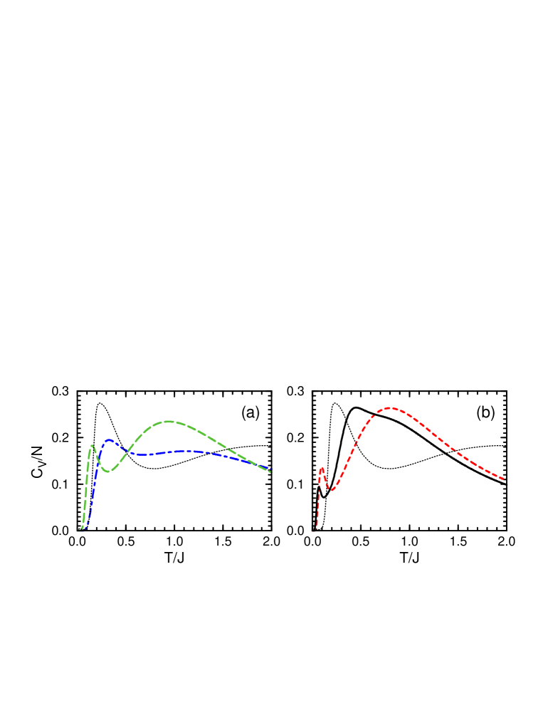
Figure 1: Heat capacities as functions of temperature for $\alpha=\frac{1}{2}$ for the compass clusters $L\times L$ of sizes $L=2,3$ (panel (a), dashed-dotted and long-dashed lines) and $L=4,5$ (panel (b), dashed and solid lines) and for the compass ladder of $104$ spins (black dotted line).

Table 1: Ground state energy $E_{0}$ and first excited state energy $E_{1}$ and their degeneracies $d$ for $10$ nonequivalent subspaces of the $5\times 5$ compass model (1) at $\alpha=1/2$.

$n\!$	1	2	3	4	5	6	7	8	9	10
$\!E_{0}\!\!$	$-14.54\!$	$-14.31\!$	$-14.30\!$	$-14.22\!$	$-13.75\!$	$-13.67\!$	$-13.52\!$	$-13.45\!$	$-13.22\!$	$-12.79\!\!$
$\!E_{1}\!\!$	$-13.80\!$	$-13.15\!$	$-12.91\!$	$-12.50\!$	$-12.86\!$	$-12.99\!$	$-13.26\!$	$-12.67\!$	$-12.88\!$	$-12.30\!\!$
$d\!$	2	20	20	20	50	100	50	100	100	50

Kernel Polynomial Method is based on the expansion into the series of Chebyshev polynomials [9]. Chebyshev polynomial of the $n$-th degree is defined as $T_{n}(x)=\cos[n\arccos x]$ where $x\in[-1,1]$ and $n$ is integer. Further on we are going to calculate $T_{n}$ of the Hamiltonian so first we need to renormalize it so that its spectrum fits the interval $[-1,1]$. This can be done easily if we know the width of the spectrum. Our aim is to calculate the renormalized density of states $\tilde{\rho}(E)$ given by $\tilde{\rho}(E)=(1/D)\sum_{n=0}^{D-1}\delta(E-\tilde{E_{n}})$, where the sum is over eigenstates of ${\cal H}(\alpha)$ and $D$ is the dimension of the Hilbert space. The moments $\mu_{n}$ of the expansion of $\tilde{\rho}(E)$ in basis of Chebyshev polynomials can be expressed by

$$\mu_{n}=\int_{-1}^{1}T_{n}(E)\tilde{\rho}(E)dE=\frac{1}{D}\Tr\{T_{n}(\tilde{\cal{H}})\}\,.$$ (3)

Trace can be efficiently estimated using stochastic approximation:

$$\Tr\,\{T_{n}(\tilde{\cal{H}})\}\approx\frac{1}{R}\sum_{r=1}^{R}\;\langle r|T_{n}(\tilde{{\cal H}})|r\rangle\,,$$ (4)

where $|r\rangle$ ($r=1,2,\dots,R$) are randomly picked complex vectors with components $\chi_{r,k}$ ($k=1,2,\dots,D$) satisfying $\langle\chi_{r,k}\rangle=0$, $\langle\chi_{r,k}\chi_{r^{\prime},l}\rangle=0$, $\langle\bar{\chi}_{r,k}\chi_{r^{\prime},l}\rangle=\delta_{r,r^{\prime}}\delta_{k,l}$ (average is taken over the probability distribution). This approximation converges very rapidly to the true value of the trace, especially for large $D$. Action of the $T_{n}(\tilde{\cal{H}})$ operator on a vector $|r\rangle$ can be determined recursively using the following relation between Chebyshev polynomials: $T_{n}(\tilde{\cal H})|r\rangle=\{2\tilde{\cal H}\,T_{n-1}(\tilde{\cal H})-T_{n-2}(\tilde{\cal H})\}|r\rangle$. We can also use the relation $2T_{m}(x)T_{n}(x)=T_{m+n}(x)+T_{m-n}(x)$ to get moments $\mu_{2n}$ from the polynomials of the degree $n$. Finally the required function,

$$\tilde{\rho}(E)\approx\frac{1}{\pi\sqrt{1-E^{2}}}\left\{g_{0}\mu_{0}+2\sum_{n=1}^{N-1}g_{n}\mu_{n}T_{n}(E)\right\}\,,$$ (5)

can be reconstructed from the $N$ known moments, where $g_{n}$ coefficients come from the integral kernel we use for better convergence. Here we use Jackson kernel. Choosing the arguments of $\tilde{\rho}(E)$ as being equal to $E_{k}=\cos[(2k-1)\pi/2N^{\prime}]$ ($k=1,2,\dots,N^{\prime}$) we can change the last formula into a cosine Fourier series and use Fast Fourier Transform algorithms to obtain rapidly $\tilde{\rho}(E_{k})$. This point is crucial when $N$ and $N^{\prime}$ are large, which is the case here; our choice will be $N=20000$ and $N^{\prime}=2N$. In such a way we can get the density of states for $4\times 4$ and $5\times 5$ systems. In the latter case we obtain $10$ energy spectra for $10$ nonequivalent subspaces — these can be summed up with proper degeneracy factors (see table 1) to get the final density of states $\tilde{\rho}(E)$ and next the partition function via rescaling and numerical integration.

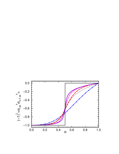
Figure 2: Correlations $\langle\sigma^{x}_{i,w}\sigma^{x}_{i+1,w}\rangle$ in the ground state calculated for sizes $L=2,3,4,5$ (dashed-dotted, long-dashed, dashed and solid line) and for infinite ladder (black dotted line) as functions of $\alpha$. Step function shows a discontinuous transition for a classical compass model at $\alpha=1/2$.

The heat capacity $C_{V}$ for the compass $L\times L$ clusters behaves differently from that for a compass ladder, see heat. The main difference is vanishing of the low–$T$ peak when the system’s size increases. This correspond to vanishing of the low–energy modes which is consistent with presence of the ordered phase for finite $T$ in the thermodynamic limit. In contrast, heat capacity of the ladder indicates robust low–energy excitations and dense excitation spectrum at higher energies causing a broad peak in $C_{V}$.

In cor we compare nearest neighbor correlations as functions of $\alpha$ for finite clusters, infinite compass ladder and classical compass model on a square lattice. Curves for finite clusters converge to certain final functions which is something intermediate between classical case and quantum ladder. This result shows that even in large $L$ limit the 2D compass model preserves quantum correction to a classical behavior even though it chooses ordering in one direction [3].

In summary, we have shown that exact heat capacities of square compass $L\times L$ clusters could be obtained by implementing the symmetries up to $L=5$. The behavior of the low–$T$ peak in the heat capacity indicates that the gap in the spectrum decreases with increasing $L$. This agrees with the numerical results obtained before by numerical approach [2].

We acknowledge support by the Foundation for Polish Science (FNP) and by the Polish Ministry of Science and Higher Education under Project No. N202 068 32/1481.

References

References

- [1] Douçot B, Feigel man M V, Ioffe L B and Ioselevich A S 2005 Phys. Rev. B 71 024505
- [2] Dorier J, Becca F and Mila F 2005 Phys. Rev. B 72 024448
- [3] Wenzel S and Janke W 2008 Phys. Rev. B 78 064402
- [4] Vidal G 2007 Phys. Rev. Lett. 99 220405
- [5] Cincio L, Dziarmaga J and Rams M M 2008 Phys. Rev. Lett. 100 240603
- [6] Brzezicki W, Dziarmaga J and Oleś A M 2007 Phys. Rev. B 75 134415
- [7] Eriksson E and Johannesson H 2009 Preprint arXiv:0903.1682
- [8] Brzezicki W and Oleś A M 2009 Phys. Rev. B 80 submitted
- [9] Weisse A and Fehske H 2008 Computational Many Particle Physics Lect. Notes Phys. vol 739, ed H Fehske, R Schneider and A Weisse (Berlin: Springer) pp 545 -77