Path integral approach to Asian options in the Black-Scholes model

Abstract

We derive a closed-form solution for the price of an average price as well as an average strike geometric Asian option, by making use of the path integral formulation. Our results are compared to a numerical Monte Carlo simulation. We also develop a pricing formula for an Asian option with a barrier on a control process, combining the method of images with a partitioning of the set of paths according to the average along the path. This formula is exact when the correlation is zero, and is approximate when the correlation increases.

I Introduction

Since the beginning of financial science, stock prices, option prices and other quantities have been described by stochastic and partial differential equations. Since the 1980s however, the path integral approach, created in the context of quantum mechanics by Richard Feynman Feynman (1), has been introduced to the field of finance Dash 1 (2, 3). Earlier, Norbert Wiener Wiener (4), in his studies on Brownian motion and the Langevin equation, used a type of functional integral that turns out to be a special case of the Feynman path integral (see also Mark Kac Kac (5), and for a general overview see Kleinert Kleinert (6) and Schulman Schulman (7)). The power of path-integration for finance (Kleinert (6),Rosa-Clot (8, 9, 10, 11, 12, 13, 14)) lies in its ability to naturally account for payoffs that are path-dependent. This makes path integration the method of choice to treat one of the most challenging types of derivatives, the path-dependent options. Feynman and Kleinert Feynman-Kleinert (15) showed how quantum-mechanical partition functions can be approximated by an effective classical partition function, a technique which has been successfully applied to the pricing of path-dependent options (see ref. Kleinert (6) and references therein, and Refs. Kleinert 2 (12, 16) for recent applications).

There exist many different types of path-dependent options. The two types which are considered in this paper are Asian and barrier options. Asian options are exotic path-dependent options for which the payoff depends on the average price of the underlying asset during the lifetime of the option Hull (17, 11, 18, 19). One distinguishes between average price and average strike Asian options. The average price Asian option has been treated in the context of path integrals by Linetsky Linetsky (20). The payoff of an average price is given by $\max(\bar{S}_{T}-K,0)$ and $\max(K-\bar{S}_{T},0)$ for a call and put option respectively. Here $K$ is the strike price and $\bar{S}_{T}$ denotes the average price of the underlying asset at maturity $T$. $\bar{S}_{T}$ can either be the arithmetical or geometrical average of the asset price. Average price Asian options cost less than plain vanilla options. They are useful in protecting the owner from sudden short-lasting price changes in the market, for example due to order imbalances Rosenow (21). Average strike options are characterized by the following payoffs: $\max(S_{T}-\bar{S}_{T},0)$ and $\max(\bar{S}_{T}-S_{T},0)$ for a call and put option respectively, where $S_{T}$ is the price of the underlying asset at maturity $T$. Barrier options are options with an extra boundary condition. If the asset price of such an option reaches the barrier during the lifetime of the option, the option becomes worthless, otherwise the option has the same payoff as the option on which the barrier has been imposed. (for more information on exit-time problems see Ref. Masilover (22) and the references therein)

In section II we treat the geometrically averaged Asian option. In section II.1 the asset price propagator for this standard Asian option is derived within the path integral framework in a similar fashion as in Ref. Linetsky (20) for the weighted Asian option. The underlying principle of this derivation is the effective classical partition function technique developed by Feynman and Kleinert Feynman-Kleinert (15). In section II.2 we present an alternative derivation of this propagator using a stochastic calculus approach. This propagator now allows us to price both the average price and average strike Asian option. For both types of options this results in a pricing formula which is of the same form as the Black-Scholes formula for the plain vanilla option. Our result for the option price of an average price Asian option confirms the result found in the literature Linetsky (20, 23). For the average strike option no formula of this simplicity exists as far as we know. Our derivation and analysis of this formula is presented in section II.3, where our result is checked with a Monte Carlo simulation. In section III we impose a boundary condition on the Asian option in the form of a barrier on a control process, and check whether the method used in section II is still valid when this boundary condition is imposed on the propagator for the normal Asian option, using the method of images. Finally in Section IV we draw conclusions.

II Geometric Asian options in the Black-Scholes model

II.1 Partitioning the set of all paths

The path integral propagator is used in financial science to track the probability distribution of the logreturn $x_{t}=\log(S_{t}/S_{0})$ at time $t$, where $S_{0}$ is the initial value of the underlying asset. This propagator is calculated as a weighted sum over all paths from the initial value $x_{0}=0$ at time $t=0$ to a final value $x_{T}=\log(S_{T}/S_{0})$ at time $t=T:$

$$\mathcal{K}\left(x_{T},T|0,0\right)=\int\mathcal{D}x\text{ }\exp\left(-\int_{0}^{T}\mathcal{L}_{BS}\left[x(t)\right]\,dt\right)$$ (1)

The weight of a path, in the Black-Scholes model, is determined by the Lagrangian

$$\mathcal{L}_{BS}\left[x(t)\right]=\frac{1}{2\sigma^{2}}\left[\dot{x}-\left(\mu-\frac{\sigma^{2}}{2}\right)\right]^{2}$$ (2)

where $\mu$ is the drift and $\sigma$ is the volatility appearing in the Wiener process for the logreturn Rosa-Clot (8).

For Asian options, the payoff is a function of the average value of the asset. Therefore we introduce $\bar{x}_{T}=\log\left(\bar{S}_{T}/S_{0}\right)$ as the logreturn corresponding to the average asset price at maturity $T$. When $\bar{S}_{T}$ is the geometric average of the asset price, then $\bar{x}_{T}$ is an algebraic average.

$$\bar{x}_{T}=\frac{1}{T}\int_{0}^{T}x(t)dt.$$ (3)

The key step to treat Asian options within the path integral framework is to partition the set of all paths into subsets of paths, where each path in a given subset has the same average $\bar{x}_{T}$. Summing over only these paths that have a given average $\bar{x}_{T}$ defines the conditional propagator $\mathcal{K}\left(x_{T},T\,\left|0,0\right|\bar{x}_{T}\right)$:

$$\mathcal{K}\left(x_{T},T\,\left|0,0\right|\bar{x}_{T}\right)=\int\mathcal{D}x\,\delta\left(\bar{x}_{T}-\frac{1}{T}\int_{0}^{T}x(t)\,dt\right)\exp\left(-\int_{0}^{T}\mathcal{L}_{BS}\left[x(t)\right]\,dt\right)$$ (4)

This is indeed a partitioning of the sum over all paths:

$$\mathcal{K}\left(x_{T},T|0,0\right)={\displaystyle\int\limits_{-\infty}^{\infty}}d\bar{x}_{T}\text{ }\mathcal{K}\left(x_{T},T\,\left|0,0\right|\bar{x}_{T}\right)$$ (5)

The delta function in the sum $\int\mathcal{D}x$ over all paths picks out precisely all the paths that will have the same payoff for an Asian option.

The calculation of $\mathcal{K}\left(x_{T},T\,\left|0,0\right|\bar{x}_{T}\right)$ is straightforward; when the delta function is rewritten as an exponential,

$$\mathcal{K}\left(x_{T},T\,\left|0,0\right|\bar{x}_{T}\right)={\displaystyle\int\limits_{-\infty}^{\infty}}\frac{dk}{2\pi}e^{ikx}\int\mathcal{D}x\,\exp\left(-\int_{0}^{T}\left(\mathcal{L}_{BS}\left[x(t)\right]+\frac{1}{T}ikx(t)\right)dt\right),$$ (6)

the resulting Lagrangian is that of a free particle in a constant force field in 1D. The resulting integration over paths is found by standard procedures Feynman Hibbs (24):

$$\mathcal{K}\left(x_{T},T\,\left|0,0\right|\bar{x}_{T}\right) =\frac{\sqrt{3}}{\pi\sigma^{2}T}\exp\left\{-\frac{1}{2\sigma^{2}T}\left[x_{T}-\left(\mu-\frac{\sigma^{2}}{2}\right)T\right]^{2}\right.$$

$$\left.-\frac{6}{\sigma^{2}T}\left(\bar{x}_{T}-\frac{x_{T}}{2}\right)^{2}\right\},$$ (7)

and corresponds to the result found by Kleinert Kleinert (6) and by Linetsky Linetsky (20).

II.2 Link with stochastic calculus

The conditional propagator $\mathcal{K}\left(x_{T},T\,\left|0,0\right|\bar{x}_{T}\right)$ is interpreted in the framework of stochastic calculus as the joint propagator $\mathcal{K}\left(x_{T},\bar{x}_{T},T\,|0,0,0\right)$ of $x_{T}$ and its average $\bar{x}_{T}$. The calculation of $\mathcal{K}\left(x_{T},\bar{x}_{T},T\,|0,0,0\right)$ here is similar to the derivation presented in Ref. Glassy (25) where this joint propagator is calculated for the Vasicek model. The main point is that in a Gaussian model the joint distribution of the couple $\left\{x_{T},\bar{x}_{T}\right\}$ has to be Gaussian too. As a consequence this joint distribution is fully characterized by the expectation values and the variances of $x_{T}$ and $\bar{x}_{T}$ and by the correlation between these two processes. The expectation value of $\bar{x}_{T}\left(t\right)$ is given by $\left(\mu-\frac{\sigma^{2}}{2}\right)\frac{t}{2}$, its variance by $\frac{\sigma^{2}t}{3}$ and the correlation between the two processes by $\frac{\sqrt{3}}{2}$. The density function of such a Gaussian process is then known to be

$$\mathcal{K}\left(x_{T},\bar{x}_{T},T\,|0,0,0\right) =\frac{\sqrt{3}}{\pi\sigma^{2}T}\exp\left(-\frac{2}{\sigma^{2}T}\left\{\left[x_{T}-\left(\mu-\frac{\sigma^{2}}{2}\right)T\right]^{2}+3\left[\bar{x}_{T}-\left(\mu-\frac{\sigma^{2}}{2}\right)\frac{T}{2}\right]^{2}\right.\right.$$

$$\left.\left.-3\left[x_{T}-\left(\mu-\frac{\sigma^{2}}{2}\right)T\right]\left[\bar{x}_{T}-\left(\mu-\frac{\sigma^{2}}{2}\right)\frac{T}{2}\right]\right\}\right)$$ (8)

This agrees with Eq. (7) for $\mathcal{K}\left(x_{T},T\,\left|0,0\right|\bar{x}_{T}\right)$.

II.3 Pricing of an average strike geometric Asian option

If the payoff at time $T$ of an Asian option is written as $V_{T}^{Asian}(x_{T},\bar{x}_{T})$, then the expected payoff is

$$\mathbb{E}\left[V_{T}^{Asian}(x_{T},\bar{x}_{T})\right]={\displaystyle\int\limits_{-\infty}^{\infty}}dx_{T}{\displaystyle\int\limits_{-\infty}^{\infty}}d\bar{x}_{T}\text{ }V_{T}^{Asian}(x_{T},\bar{x}_{T})\mathcal{K}\left(x_{T},T\,\left|0,0\right|\bar{x}_{T}\right)$$ (9)

The price of the option, $V_{0}^{Asian}$ is the discounted expected payoff,

$$V_{0}^{Asian}=e^{-rT}\mathbb{E}\left[V_{T}^{Asian}(x_{T},\bar{x}_{T})\right]$$ (10)

where $r$ is the discount (risk-free) interest rate. Using expression (9) the price of any option which is dependent on the average of the underlying asset during the lifetime of the option can be calculated. We will now derive the price of an average strike geometric Asian call option explicitly. In order to do this, expression (9) has to be evaluated using the payoff:

$$V_{T}^{Asian}(x_{T},\bar{x}_{T})=\max(S_{T}-\bar{S}_{T},0)=S_{0}\max(e^{x_{T}}-e^{\bar{x}_{T}},0)$$ (11)

Substituting (11) in (10) yields

$$V_{0}^{Asian}=S_{0}e^{-rT}{\displaystyle\int\limits_{-\infty}^{\infty}}d\bar{x}_{T}{\displaystyle\int\limits_{\bar{x}_{T}}^{\infty}}dx_{T}\text{ }\left(e^{x_{T}}-e^{\bar{x}_{T}}\right)\mathcal{K}\left(x_{T},T\,\left|0,0\right|\bar{x}_{T}\right)$$ (12)

where the lower boundary of the $x_{T}$ integration now depends on $\bar{x}_{T}$. When considering an average price call, the payoff (for a call option) is $\max(\bar{S}_{T}-K,0)$ leading to a constant lower boundary $\log(K/S_{0})$ for the $\bar{x}_{T}$ integration, and the integrals are easily evaluated. In the present case however, the integration boundary is more complicated and it is more convenient to express this boundary through a Heaviside function, written in its integral representation:

$$V_{0}^{Asian} =S_{0}\,e^{-rT}\,\frac{1}{2\pi i}\int_{-\infty}^{+\infty}d\bar{x}_{T}\,\,\int_{-\infty}^{+\infty}dx_{T}\int_{-\infty}^{+\infty}d\tau\,\frac{e^{i\left(x_{T}-\bar{x}_{T}\right)\tau}}{\tau-i\varepsilon}$$ (13)

$$\times\left(e^{x_{T}}-e^{\bar{x}_{T}}\right)\mathcal{K}\left(x_{T},T\,\left|0,0\right|\bar{x}_{T}\right)$$

Now the two original integrals have been reduced to Gaussians at the cost of inserting a complex term in the exponential. Expression (13) can be split into two terms denoted $I_{1}$ and $I_{2}$, where

$$I_{1} =S_{0}e^{-rT}\frac{\sqrt{3}}{\pi\sigma^{2}T}\,\frac{1}{2\pi i}\int_{-\infty}^{+\infty}d\tau\frac{1}{\tau-i\varepsilon}\int_{-\infty}^{+\infty}d\bar{x}_{T}\int_{-\infty}^{+\infty}dx_{T}$$

$$\times\exp\left\{-\frac{1}{2\sigma^{2}T}\left[x_{T}-\left(\mu-\frac{\sigma^{2}}{2}\right)T\right]^{2}\right.$$

$$\left.-\frac{6}{\sigma^{2}T}\left(\bar{x}_{T}-\frac{x_{T}}{2}\right)^{2}+i\left(x_{T}-\bar{x}_{T}\right)\tau+x_{T}\right\}$$ (14)

and $I_{2}$ has the same form, except with $\bar{x}_{T}$ instead of $x_{T}$ in the last term of the argument of the exponent. As a first step, the Gaussian integrals over $x_{T}$ and $\bar{x}_{T}$ are calculated, yielding

$$I_{1}=S_{0}\,e^{-\left(r-\mu\right)T}\frac{1}{2\pi i}\int_{-\infty}^{+\infty}\frac{f\left(\tau\right)}{\tau-i\varepsilon}d\tau$$ (15)

with

$$f\left(\tau\right)=\exp\left[-\frac{\sigma^{2}T}{6}\tau^{2}+\left(\mu+\frac{\sigma^{2}}{2}\right)\frac{iT}{2}\tau\right]$$ (16)

Now the integral has been reduced to a form which can be rewritten by making use of Plemelj’s formulae. Taking into account symmetry, this reduces to

$$\int_{-\infty}^{+\infty}\frac{f\left(\tau\right)}{\tau-i\varepsilon}d\tau=i\pi\left[\operatorname{erf}\left(\frac{b}{2\sqrt{a}}\right)+1\right]$$ (17)

with

$$\left\{\begin{array}[c]{l}\vskip 3.0pt plus 1.0pt minus 1.0pta=\dfrac{\sigma^{2}T}{6}\\ \vskip 3.0pt plus 1.0pt minus 1.0ptb=\left(\mu+\dfrac{\sigma^{2}}{2}\right)\dfrac{T}{2}\end{array}\right.$$ (18)

The first term thus becomes

$$I_{1}=S_{0}e^{-rT}\frac{\sqrt{3}}{\pi\sigma^{2}T}\,\frac{1}{2}\left\{\operatorname{erf}\left[\sqrt{\frac{3T}{8\sigma^{2}}}\left(\mu+\frac{\sigma^{2}}{2}\right)\right]+1\right\}$$ (19)

The second term, $I_{2},$ is evaluated similarly, leading to

$$V_{0}^{Asian} =S_{0}e^{-rT}\left(\frac{\sqrt{3}}{\pi\sigma^{2}T}\,\frac{1}{2}\left\{\operatorname{erf}\left[\sqrt{\frac{3T}{8\sigma^{2}}}\left(\mu+\frac{\sigma^{2}}{2}\right)\right]+1\right\}\right.$$

$$\left.-\exp\left[\left(\mu-\frac{\sigma^{2}}{6}\right)\frac{T}{2}\right]\left\{\operatorname{erf}\left[\sqrt{\frac{3T}{8\sigma^{2}}}\left(\mu-\frac{\sigma^{2}}{6}\right)\right]+1\right\}\right)$$ (20)

Using the cumulative distribution function of the normal distribution

$$\Phi\left(x\right)=\nolinebreak\frac{1}{2}\left[1+\operatorname{erf}\left(\frac{x}{\sqrt{2}}\right)\right]$$ (21)

this can be rewritten in a more compact form as

$$V_{0}^{Asian}=S_{0}e^{-rT}\left(e^{\mu T}\,\,\Phi\left(d_{1}\right)-e^{\left(\mu-\frac{\sigma^{2}}{6}\right)\frac{T}{2}}\Phi\left(d_{2}\right)\right)$$ (22)

with the following shorthand notations

$$\left\{\begin{array}[c]{c}\vskip 3.0pt plus 1.0pt minus 1.0ptd_{1}=\sqrt{\dfrac{3T}{4\sigma^{2}}}\left(\mu+\dfrac{\sigma^{2}}{2}\right)\\ \vskip 3.0pt plus 1.0pt minus 1.0ptd_{2}=\sqrt{\dfrac{3T}{4\sigma^{2}}}\left(\mu-\dfrac{\sigma^{2}}{6}\right)\end{array}\right.$$ (23)

Expression (22) is the analytic pricing formula for an average strike geometric Asian call option, obtained in the present work with the path integral formalism. To the best of our knowledge, no pricing formula of this simplicity exists. To check this formula, we compared its results to those of a Monte Carlo simulation. The Monte Carlo scheme used is as follows Glassy (25): first, the evolution of the logreturn is simulated for a large number of paths. This evolution is governed by a discrete geometric Brownian motion for a number of time steps. Using the value for the logreturn at each time step, the average logreturn can be calculated for every path. Subsequently the payoff per path can be obtained, which is then used to calculate the option price by averaging over all payoffs per path en discounting back in time. The analytical result and the Monte Carlo simulation agree to within a relative error of 0.3% when 500 000 samples and 100 time steps are used. This means that our analytical result lies within the error bars at every point. We also obtained the result for an average price Asian option; in contrast to the new result for the average strike option this could be compared to the existing formula Linetsky (20, 23), and was found to be the same.

III Asian option with a barrier on a control process

III.1 Derivation of the option price

In this case we consider two stochastic processes:

$$\left\{\begin{array}[c]{l}\vskip 3.0pt plus 1.0pt minus 1.0ptdx=\left(\mu-\dfrac{\sigma^{2}}{2}\right)dt+\sigma dW_{1}\\ \vskip 3.0pt plus 1.0pt minus 1.0ptdy=\left(\nu-\dfrac{\xi^{2}}{2}\right)dt+\xi dZ\end{array}\right.$$ (24)

which are correlated in the following manner: $\left\langle dW_{1}dZ\right\rangle=\rho dt$. The $x$ process models the logreturn of the asset price which underlies the Asian option, and the $y$ process describes the control process. The payoff for an Asian option with a barrier on a control process is the same as for a normal Asian option, with the extra condition that the payoff is zero whenever the value of $\allowbreak y$ surpasses a certain predetermined barrier. This is an example of an up-and-out barrier. There are other types of barrier options, namely down-and-out etc., but since their treatment is analogous we will not consider them here. The payoff for an Asian option with a barrier on a control process is given by:

$$V_{T}^{AB}(x_{T},\bar{x}_{T})=\left\{\begin{array}[c]{l}S_{0x}e^{\bar{x}_{T}}-K\text{ \ \ \ \ }\forall t\in\left[0,T\right]:y\left(t\right)<y_{B}\\ \leavevmode\nobreak\ \ \ 0\text{ \ \leavevmode\nobreak\ \leavevmode\nobreak\ \leavevmode\nobreak\ \leavevmode\nobreak\ \ \ \leavevmode\nobreak\ \leavevmode\nobreak\ \leavevmode\nobreak\ \ \leavevmode\nobreak\ \leavevmode\nobreak\ \leavevmode\nobreak\ \leavevmode\nobreak\ }\exists t\in\left[0,T\right]:y\left(t\right)\geq y_{B}\end{array}\right.$$ (25)

where the payoff of an average price Asian option has been used. Here $S_{0x}$ denotes the initial asset price of the asset corresponding to the logreturn $x$ and $y_{B}$ is the value of the barrier which has been placed upon the $y$ process. It is difficult to price this option using payoff (25) because of the extra barrier condition. However, if this condition could somehow be included in the propagator for these two processes, then the payoff would reduce to that of a normal (average price) Asian option, making the calculations more tractable. To construct this new propagator, henceforth called barrier-propagator, a linear combination of propagators for the combined evolution of both processes given in (24) can be taken:

$$\mathcal{K}_{y}^{B}\left(x_{T},y_{T},\bar{x}_{T},T\,|0,0,0,0\right)=\mathcal{K}\left(x_{T},y_{T},\bar{x}_{T},T\,|0,0,0,0\right)+C\leavevmode\nobreak\ \mathcal{K}\left(x_{T},y_{T},\bar{x}_{T},T\,|x_{S},y_{S},\bar{x}_{S},0\right)$$ (26)

where $\mathcal{K}_{y}^{B}$ stands for the propagator for the processes $x$ and $y$ where a barrier condition has been placed upon the $y$ process. The propagator $\mathcal{K}\left(x_{T},y_{T},\bar{x}_{T},T\,|0,0,0,0\right)$ belonging to the system (24) is an extension of the propagator (7), and is given by:

$$\mathcal{K}\left(x_{T},y_{T},\bar{x}_{T},T\,|0,0,0,0\right) =\sqrt{\frac{3}{2\pi^{3}T^{3}\sigma^{4}\xi^{2}\left(1-\rho^{2}\right)}}$$

$$\times\exp\left\{\frac{\rho}{\sigma\xi\left(1-\rho^{2}\right)T}\left[x_{T}-\left(\mu-\frac{\sigma^{2}}{2}\right)T\right]\left[y_{T}-\left(\nu-\frac{\xi^{2}}{2}\right)T\right]\right.$$

$$-\frac{1}{2\sigma^{2}\left(1-\rho^{2}\right)T}\left[x_{T}-\left(\mu-\frac{\sigma^{2}}{2}\right)T\right]^{2}-\frac{1}{2\xi^{2}\left(1-\rho^{2}\right)T}$$

$$\left.\times\left[y_{T}-\left(\nu-\frac{\xi^{2}}{2}\right)T\right]^{2}-\frac{6}{\sigma^{2}T}\left(\bar{x}_{T}-\frac{x_{T}}{2}\right)^{2}\right\}$$ (27)

Furthermore C is a factor upon which three conditions will be placed and $x_{S},y_{S}$ represent the initial condition from which the mirror-propagator starts. This mirror-propagator is used to eliminate all paths that cross the barrier, and because the paths represented by the mirror-propagator usually have higher values than the paths represented by the propagator $\mathcal{K}\left(x_{T},y_{T},\bar{x}_{T},T\,|0,0,0,0\right)$, they have been given another average $\bar{x}_{S}$. The barrier-propagator must be zero at the boundary:

$$\mathcal{K}_{y}^{B}\left(x_{T},y_{B},\bar{x}_{T},T\,|0,0,0,0\right)=0$$ (28)

Using this boundary condition, an expression for C can be derived which must satisfy three conditions: firstly C must be independent of the averages $\bar{x}_{T}$ and $\bar{x}_{S}$, secondly it may not depend on $x_{T}$ and finally it must be time-independent. This eventually leads to the following propagator for the total system of correlated stochastic processes $x$ and $y$, with a barrier condition on $y$ when $y_{T}\in\left[-\infty,y_{B}\right[$:

$$\mathcal{K}_{y}^{B}\left(x_{T},y_{T},\bar{x}_{T},T\,|0,0,0,0\right) =\mathcal{K}\left(x_{T},y_{T},\bar{x}_{T},T\,|0,0,0,0\right)$$

$$-e^{\frac{2y_{B}}{\xi\left(4-3\rho^{2}\right)}\left[\frac{4}{\xi}\left(\nu-\frac{\xi^{2}}{2}\right)-3\frac{\rho}{\sigma}\left(\mu-\frac{\sigma^{2}}{2}\right)\right]}\leavevmode\nobreak\ \mathcal{K}\left(x_{S},y_{S},\bar{x}_{S},T\,|0,0,0,0\right)$$ (29)

with the following shorthand notations:

$$\left\{\begin{array}[c]{l}x_{S}=\dfrac{2y_{B}}{\xi}\allowbreak\dfrac{\rho\sigma}{\left(4-3\rho^{2}\right)}\\ \bar{x}_{S}=\dfrac{-\left(x_{S}-x_{T}\right)+\sqrt{\left(x_{S}-x_{T}\right)^{2}+4\leavevmode\nobreak\ \bar{x}_{T}\left(\bar{x}_{T}-x_{T}\right)}}{2}\\ y_{S}=2y_{B}\end{array}\right.\vskip 6.0pt plus 2.0pt minus 2.0pt$$ (30)

The propagator (29) is equal to zero when $y_{T}\in\left[y_{B},+\infty\right]$. A graphical presentation of propagator (29) is shown in Fig. 1.

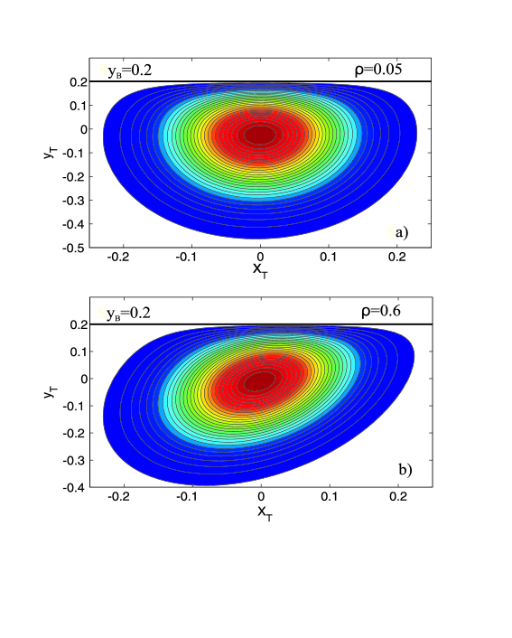
Figure 1: Graphical representation of the barrier-propagator (29) in arbitrary units, for the system of two correlated processes $x$ and $y$, given by (24), where a barrier has been placed on the $y$ process at $y_{B}=0.2$. The following values were used in this figure: $\mu=\nu=0.03\$Year${}^{-1};\sigma=\xi=0.25\leavevmode\nobreak\$Year${}^{-\frac{1}{2}};T=1\leavevmode\nobreak\$Year

Using the propagator (29) the price of an Asian option with a barrier $V_{0}^{AB}$ can be calculated. The general pricing formula is given by:

$$V_{0}^{AB}=e^{-rT}\int_{-\infty}^{y_{B}}dy_{T}\,\int_{-\infty}^{+\infty}d\bar{x}_{T}\,\,\int_{-\infty}^{+\infty}dx_{T}\,\mathcal{K}_{y}^{B}\left(x_{T},y_{T},\bar{x}_{T},T\,|0,0,0,0\right)\,V_{T}^{Asian}(x_{T},\bar{x}_{T})$$ (31)

This calculation was done for an average price option: $V_{T}^{Asian}(x_{T},\bar{x}_{T})=\max\left(S_{0x}e^{\bar{x}_{T}}-K,0\right)$. The calculation, though rather cumbersome, is essentially the same as for the Asian options in section II. The integral over $x_{T}$ is a Gaussian integral, and the remaining two integrals can be transformed into a standard bivariate cumulative normal distribution, defined by:

$$N[a,b;\chi]=\frac{1}{2\pi\sqrt{1-\chi^{2}}}\int_{-\infty}^{a}\int_{-\infty}^{b}\exp\left(-\frac{1}{2\left(1-\chi^{2}\right)}\left(x^{2}+y^{2}-2\chi xy\right)\right)dxdy$$ (32)

This eventually leads to the following pricing formula for an Asian option with a barrier:

$$V_{0}^{AB} =e^{-rT}\left[S_{0x}e^{\frac{T}{2}\left(\mu-\frac{\sigma^{2}}{6}\right)}N\left(d_{1},d_{2},-\sqrt{\frac{3}{4}}\rho\right)-K\leavevmode\nobreak\ N\left(d_{3},d_{4},-\sqrt{\frac{3}{4}}\rho\right)\right.$$

$$-S_{0x}\leavevmode\nobreak\ e^{\frac{3T}{\sigma^{2}}\left(\frac{x_{S}}{T}+\frac{\sigma^{2}}{6}\right)\left[2\frac{x_{S}}{T}+\left(\mu-\frac{\sigma^{2}}{6}\right)\right]}\left(\frac{B}{S_{0y}}\right)^{\frac{2\left[\frac{4}{\xi}\left(\nu-\frac{\xi^{2}}{2}\right)-3\frac{\rho}{\sigma}\left(\mu-\frac{\sigma^{2}}{2}\right)\right]}{\xi\left(4-3\rho^{2}\right)}}N\left(d_{5},d_{6},-\sqrt{\frac{3}{4}}\rho\right)$$

$$\left.+K\leavevmode\nobreak\ e^{\frac{3}{\sigma^{2}}x_{S}\left[\frac{2x_{S}}{T}+\left(\mu-\frac{\sigma^{2}}{2}\right)\right]}\left(\frac{B}{S_{0y}}\right)^{\frac{2\left[\frac{4}{\xi}\left(\nu-\frac{\xi^{2}}{2}\right)-3\frac{\rho}{\sigma}\left(\mu-\frac{\sigma^{2}}{2}\right)\right]}{\xi\left(4-3\rho^{2}\right)}}N\left(d_{7},d_{8},-\sqrt{\frac{3}{4}}\rho\right)\right]$$ (33)

where the following shorthand notations were used:

$$\begin{array}[c]{l}d_{1}=-\dfrac{\ln\left(\dfrac{K}{S_{0x}}\right)-\dfrac{T}{2}\left(\mu+\dfrac{\sigma^{2}}{6}\right)}{\sqrt{\dfrac{\sigma^{2}T}{3}}}\\ d_{2}=\dfrac{\ln\left(\dfrac{B}{S_{0y}}\right)-T\left(\nu-\dfrac{\xi^{2}}{2}+\dfrac{\sigma\xi\rho}{2}\right)}{\sqrt{\xi^{2}T}}\\ d_{3}=-\dfrac{\ln\left(\dfrac{K}{S_{0x}}\right)-\dfrac{T}{2}\left(\mu-\dfrac{\sigma^{2}}{2}\right)}{\sqrt{\dfrac{\sigma^{2}T}{3}}}\\ d_{4}=\dfrac{\ln\left(\dfrac{B}{S_{0y}}\right)-T\left(\nu-\dfrac{\xi^{2}}{2}\right)}{\sqrt{\xi^{2}T}}\\ d_{5}=-\dfrac{\ln\left(\dfrac{K}{S_{0x}}\right)-T\left[2\dfrac{x_{S}}{T}+\dfrac{1}{2}\left(\mu+\dfrac{\sigma^{2}}{6}\right)\right]}{\sqrt{\dfrac{\sigma^{2}T}{3}}}\\ d_{6}=\dfrac{\ln\left(\dfrac{B}{S_{0y}}\right)-\dfrac{T}{\sigma}\left[3\xi\rho\dfrac{x_{S}}{T}+\sigma\dfrac{x_{S}}{T}+\sigma\left(\nu-\dfrac{\xi^{2}}{2}+\dfrac{\sigma\xi\rho}{2}\right)\right]}{\sqrt{\xi^{2}T}}\\ d_{7}=-\dfrac{\ln\left(\dfrac{K}{S_{0x}}\right)-T\left[\dfrac{2x_{S}}{T}+\dfrac{1}{2}\left(\mu-\dfrac{\sigma^{2}}{2}\right)\right]}{\sqrt{\dfrac{\sigma^{2}T}{3}}}\\ d_{8}=\dfrac{\ln\left(\dfrac{B}{S_{0y}}\right)-\dfrac{T}{2\sigma}\left[\dfrac{1}{T}\left(6\rho x_{S}\xi+2\sigma y_{S}\right)+2\sigma\left(\nu-\dfrac{\xi^{2}}{2}\right)\right]}{\sqrt{\xi^{2}T}}\end{array}$$ (34)

III.2 Results and discussion

Fig. (2) shows the option price for an Asian option with a barrier as a function of the initial asset price belonging to the $y$ process, defined by: $S_{Ty}=S_{0y}e^{y_{T}}$.

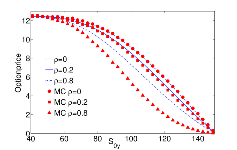
Figure 2: Option price for an Asian option with a barrier, as a function of the initial asset price belonging to the $y$ process. Since no specific asset is considered the option price could be stated in any currency, therefore this figure is given in arbitrary units. The analytical result deviates from the Monte Carlo simulation (MC) for increasing correlation. The value for the barrier used in this figure is $B=150\text{.}$

This figure shows that the analytical result derived in section III.1 deviates from the Monte Carlo simulation with increasing correlation. The approximate nature of our approach can be understood as follows. The essence of the approach presented here is that to calculate the price of Asian barrier options, two steps need to be taken. First, a partitioning of paths according to the average along the path must be performed, and second, the method of images must be used in order to cancel out paths which have reached the barrier. The difficulty combining these two steps, is that mirror paths have a different average than the original paths, and thus belong to a different partition. This difficulty can apparently be overcome by treating the average itself as a separate, correlated process (as proposed in Ref. Glassy (25)). This procedure, relating $\mathcal{K}\left(x_{T},T\,\left|0,0\right|\bar{x}_{T}\right)$ to $\mathcal{K}\left(x_{T},\bar{x}_{T},T\,|0,0,0\right)$, leads to the correct propagator (and price) in the case of a plain Asian option as shown in section II.2.

However, from the results shown in Fig. 2 it is clear that this is no longer the case for an Asian option with a barrier on a correlated control process. This is because the exact average of the $x$ process does not behave as a separate, correlated process (the average described by this process is henceforth called the approximate average). This approach is exact for a plain Asian option, where all paths contribute, but when a barrier is implemented using the method of images, and thus eliminating some of the paths, the following approximation is made. When the $y$ process hits the barrier and is thus eliminated, its corresponding $x$ and $\bar{x}$ processes are eliminated as well. But the $\bar{x}$ process considered in our derivation is only approximate, so the wrong $\bar{x}$ paths are eliminated. The central question is whether this will lead to a difference between the distribution of contributing paths for the exact averages and the corresponding distribution for the approximate averages, when a barrier has been implemented. Figure 3 shows that this is indeed the case, and that this difference increases when correlation increases.

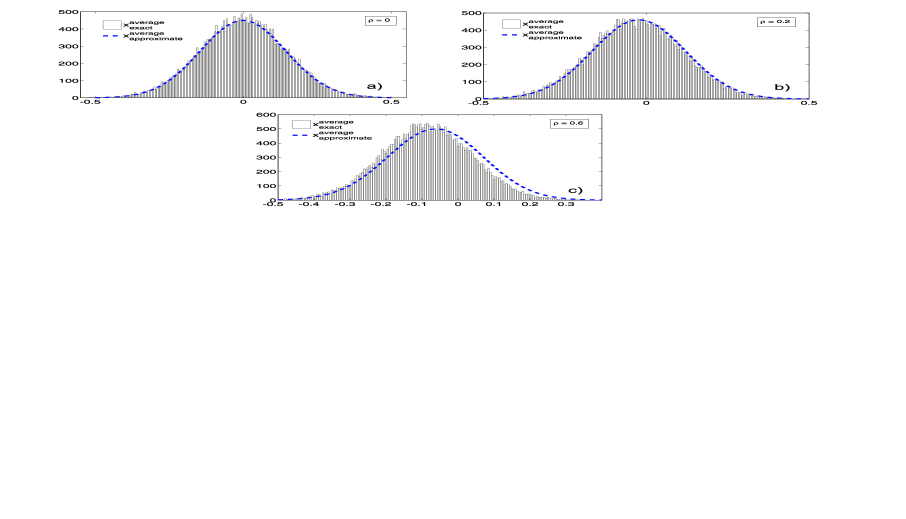
Figure 3: Comparison of the distribution of the exact and the approximate average of the logreturn $x$, when a barrier is present. a) When the correlation equals zero, both distributions are equal b) For relative small values of the correlation, the assumption that the $\bar{x}$ process is correlated with the process for the logreturn $x$ is still relatively good.  c) When the correlation is relatively large, the distribution of the exact averages deviates significantly from the approximate averages.

When the correlation is zero, the paths which are eliminated for both the exact and the approximate average are randomly distributed (because the behavior of $\bar{x}$ has nothing to do with the behavior of $y$) , which means that both distributions remain the same Gaussian as they would be without a barrier. This is the reason why our result is exact when correlation is zero. Another source of approximation lies in the use of the Black-Scholes model which has well-known limitations Bouchaud (14, 17). Several other types of market models propose to overcome such limitations, for example by introducing additional ad hoc stochastic variables Heston (26) or by improving the description of the behavior of buyers/sellers Medo (27). The extension of the present work to for example the Heston model lies beyond the scope of this article.

IV Conclusions

In this paper, we derived a closed-form pricing formula for an average price as well as an average strike geometric Asian option within the path integral framework. The result for the average price Asian option corresponds to that found by Linetsky Linetsky (20), using the effective classical partition function technique developed by Feynman and Kleinert Feynman-Kleinert (15). The result for the average strike Asian option was compared to a Monte Carlo simulation. We found that the agreement between the numerical simulation and the analytical result for an average strike Asian option is such that they coincide to within a relative error of less than 0.3 % for at least 500 000 samples and 100 time steps.

Furthermore, a pricing formula for an Asian option with a barrier on a control process was developed. This is an Asian option with the additional condition that the payoff is zero whenever the value of the control process crosses a certain predetermined barrier. The pricing of this option was performed by constructing a new propagator which consisted of a linear combination of two propagators for a regular Asian option. The resulting pricing formula is exact when the correlation is zero, and is approximate when the correlation increases. The central approximation made in our derivation, is that the process for the average logreturn $\bar{x}$ is treated as a stochastic process, which is correlated with the process of the logreturn $x$. This assumption is correct whenever all price-paths contribute to the total sum, but becomes approximate when a boundary condition is applied.

- (1) R.P. Feynman, Space-time approach to non-relativistic quantum mechanics, Reviews of Modern Physics 20 (1948) 367 387.
- (2) J. Dash, Path integrals and options - I, CNRS Preprint CPT-88/PE.2206, 1988.
- (3) J. Dash, Path integrals and options - II, CNRS Preprint CPT-89/PE.2333, 1989.
- (4) N. Wiener, The average of an analytical functional, Proceedings of the National Academy of Sciences 7 (1921) 253 260.
- (5) M. Kac, Wiener and integration in function spaces, American Mathematical Society. Bulletin. New Series 72 (1966) 52 68.
- (6) H. Kleinert, Path Integrals in Quantum Mechanics, Statistics, Polymer Physics, and Financial Markets, 5th edition, World Scientific Publishing Co., Singapore, 2009, pp. 1 1547.
- (7) L.S. Schulman, Techniques and Applications of Path Integration, John Wiley & Sons, Inc., 1981.
- (8) M. Rosa-Clot, S. Taddei, A path integral approach to derivative security pricing: I. Formalism and analytical results, International Journal of Theoretical and Applied Finance (2002).
- (9) M. Rosa-Clot, S. Taddei, A path integral approach to derivative security pricing: II. Numerical methods, Arxiv preprint cond-mat/9901279, 1999.
- (10) G. Montagna, N. Moreni, O. Nicrosini, A path integral way to option pricing, Physica A 310 (2002) 450.
- (11) G. Bormetti, G. Montagna, N. Moreni, O. Nicrosini, Pricing exotic options in a path integral approach, Quantitative Finance 6 (2006) 55.
- (12) H. Kleinert, Option pricing from path integral for non-gaussian fluctuations. Natural martingale and application to truncated Lévy distributions, Physica A 312 (2002) 217.
- (13) B.E. Baaquie, A path integral approach to option pricing with stochastic volatility: Some exact results, Journal of Physics. I France 7 (1997) 1733.
- (14) J.-P. Bouchaud, M. Potters, Theory of Financial Risks and Derivative Pricing, From Statistical Physics to Risk Management, Cambridge University Press, 2000.
- (15) R.P. Feynman, H. Kleinert, Effective classical partition functions, Physical Review A 34 (1986) 5080.
- (16) D. Lemmens, M. Wouters, J. Tempere, S. Foulon, A path integral approach to closed-form option pricing formulas with applications to stochastic volatility and interest rate models, Physical Review. E 78, 016101 (2008).
- (17) J.C. Hull, Options, Futures and Other Derivatives, 6th edition, Prentice Hall, 2006.
- (18) A.G.Z. Kemna, A.C.F. Vorst, A pricing method for options based on average asset values, Journal of Banking and Finance 14 (1990) 113 129.
- (19) S.M. Turnbull, L.M. Wakeman, A quick Algorithm for pricing European average options, Journal of Financial and Quantitative Analysis 26 (3) (1991).
- (20) V. Linetsky, The path integral approach to financial modeling and options pricing, Computational Economics 11 (1998) 129 163.
- (21) B. Rosenow, Fluctuations and market friction in financial trading, International Journal of Modern Physics C 13 (2002) 419.
- (22) J. Masoliver, J. Perello, Escape problem under stochastic volatility: The Heston model, Physical Review E 78 (2008) 056104.
- (23) A. Lipton, Mathematical Methods For Foreign Exchange: A Financial Engineer’s Approach, World Scientific Publishing, 2001.
- (24) R.P. Feynman, A.R. Hibbs, Quantum Mechanics and Path Integrals, McGraw-Hill, New York, N.Y, 1965.
- (25) P. Glasserman, Monte Carlo Methods in Financial Engineering, Springer, New York, 2004.
- (26) S.L. Heston, Review of Financial Studies 6 (1993) 327.
- (27) M. Medo, Y.-C. Zhang, Market model with heterogeneous buyers, Physica A 387 (2008).