Feynman path-integral treatment of the BEC-impurity polaron

Abstract

The description of an impurity atom in a Bose-Einstein condensate can be cast in the form of Fröhlich’s polaron Hamiltonian, where the Bogoliubov excitations play the role of the phonons. An expression for the corresponding polaronic coupling strength is derived, relating the coupling strength to the scattering lengths, the trap size and the number of Bose condensed atoms. This allows to identify several approaches to reach the strong-coupling limit for the quantum gas polarons, whereas this limit was hitherto experimentally inaccessible in solids. We apply Feynman’s path-integral method to calculate for all coupling strengths the polaronic shift in the free energy and the increase in the effective mass. The effect of temperature on these quantities is included in the description. We find similarities to the acoustic polaron results and indications of a transition between free polarons and self-trapped polarons. The prospects, based on the current theory, of investigating the polaron physics with ultracold gases are discussed for lithium atoms in a sodium condensate.

I Introduction

Quantum gases are used as an excellent testbed for many-body theory, and are particularly useful to investigate strong-coupling regimes or strongly correlated regimes that have remained out of reach in the solid statedalibardreview . The current work focuses on the physics of an impurity in a Bose-Einstein condensate (BEC), as this system opens a new and promising avenue to investigate long-standing problems in polaron theorypolaronreview . In 1952 Fröhlich, inspired by Landau’s concept of the polaron, derived a Hamiltonian that describes a charge carrier (electron, hole) interacting with its self-induced polarization, in an ionic crystal or a polar semiconductorLandau ; Frohlich . The Fröhlich polaron Hamiltonian has resisted exact analytical diagonalization since 1952 and became a laboratory to test methods of quantum field theorypolaronreview . Tomonaga’s canonical transformation was applied to study the weak coupling regime. Bogoliubov tackled the polaron strong coupling limit with one of his canonical transformations. Feynman used his path integral formalism (and an ad-hoc variational principle) to develop a superior all coupling approximation for the polaronFeynman . These studies were addressing the self-energy, the effective mass and the mobility of Fröhlich polarons. Studies of the optical absorption of a Fröhlich polaron were initiated by Evrard et al. KED for strong coupling and by Gurevich et al. Gurevich for the weak coupling limit. Devreese et al. Optipol calculated the optical absorption of the Fröhlich polaron at all coupling using Feynman path integrals and the response formalism introduced in Ref. FHIP . The results of Ref. Optipol reveal the internal excitation structure of the Fröhlich polaron that is absent in Ref. FHIP .

However the largest Fröhlich polaron coupling constant established in any solid by experiment is not large enough to reveal the rich internal excitation structure of the optical absorption predicted in Ref. Optipol . The possibility to tune the coupling strength in the BEC-impurity system presents a marvellous challenge and opportunity to experimentally reveal the internal excitation structure and its related resonances and scattering states “contained” in the Fröhlich field-theoretical polaron Hamiltonian. Quantum gases could therefore reveal important and subtle characteristics (eigenstates, resonances,…) of a Hamiltonian devised for a solid, however, that cannot be realized in a solid. The observation of the spectra of the BEC-impurity Hamiltonian at large coupling would be all the more interesting in view of recent studies of the spectrum of the Fröhlich polaron Hamiltonian with Diagrammatic Quantum Monte-Carlo numerical techniques MishchenkoPRL and with a new strong coupling model DeFilippisPRL96 that explore the validity of the Franck-Condon principle with increasing coupling strength. Similarly, the transition between quasi-free polarons and self-trapped polarons predicted for acoustic polaronsacoustipol is expected to occur in a coupling regime hitherto inaccessible in the solid state. Finally, a better understanding of the intermediate and strong-coupling regimes is needed to further elucidate the role of polarons and bipolarons in unconventional pairing mechanisms for high-temperature superconductivityalexandrov .

The Hamiltonian of an impurity in a Bose-Einstein condensate can be mapped onto the polaron Hamiltonian when the Bogoliubov approximation is validTimmermansPRL ; TimmermansPRA . The polaronic effects comes about through the coupling of the impurity with the Bogoliubov excitations, as shown in Sec. II. We apply the path-integral formalism, valid at all values of the coupling strength, to describe the polaronic effect in a condensate in Sec. III. As a concrete example, we use the parameters for a lithium impurity in a sodium condensate, and derive an expression linking the experimental parameters to a dimensionless coupling constant analogous to the Fröhlich coupling constant for electrons in polar crystals. The polaronic energy shift, the effective mass increase and the polaron radius are studied for all values of this coupling strength and at all temperatures where the Bogoliubov approximation is valid, in Sec. IV.

II The polaron Hamiltonian for an impurity in a condensate

The Hamiltonian of a single atom, in the presence of a Bose gas is given by:

$$\hat{H}=\frac{\hat{p}^{2}}{2m_{I}}+\sum_{\mathbf{k}}\varepsilon_{\mathbf{k}}\hat{a}_{\mathbf{k}}^{{\dagger}}\hat{a}_{\mathbf{k}}+\frac{1}{2}\sum_{\mathbf{k},\mathbf{k}^{\prime}\mathbf{,q}}V_{BB}(\mathbf{q})\hat{a}_{\mathbf{k}^{\prime}-\mathbf{q}}^{{\dagger}}\hat{a}_{\mathbf{k+q}}^{{\dagger}}\hat{a}_{\mathbf{k}}\hat{a}_{\mathbf{k}^{\prime}}+\sum_{\mathbf{k},\mathbf{q}}V_{IB}(\mathbf{q})\hat{\rho}_{I}(\mathbf{q})\hat{a}_{\mathbf{k}^{\prime}\mathbf{-q}}^{{\dagger}}\hat{a}_{\mathbf{k}^{\prime}}$$ (1)

The first term represents the kinetic energy of the ”impurity” atom with mass $m_{I}$. The operators $\hat{a}_{\mathbf{k}}^{{\dagger}},\hat{a}_{\mathbf{k}}$ create and annihilate a boson with mass $m_{B}$, wave number k, and energy $\varepsilon_{\mathbf{k}}=(\hbar k)^{2}/(2m_{B})-\mu$ where $\mu$ is the chemical potential. These bosons interact, and $V_{BB}(\mathbf{q})$ is the Fourier transform of the boson-boson interaction potential. The interaction between the bosonic atoms and the impurity atom is described by a potential $V_{IB}(\mathbf{q})$ coupling the boson density to the impurity density $\hat{\rho}_{I}(q)$ which can be expressed as a function of the impurity position operator $\hat{r}$ as

$$\hat{\rho}_{I}(\mathbf{q})=\int d^{3}\mathbf{r}\text{ }e^{-i\mathbf{q\cdot r}}\delta(\mathbf{r}-\mathbf{\hat{r}}).$$ (2)

Bose-Einstein condensation is realized when the single-particle density matrix has an eigenvalue $N_{0}\gg 1$ comparable to the total number of bosons PenroseOnsager . For a homogeneous condensate, this is expressed by the Bogoliubov shift Bogoliubov which transforms the Hamiltonian (1) into

$$\hat{H}=E_{GP}+N_{0}V_{IB}(\mathbf{0})+\dfrac{\hat{p}^{2}}{2m_{I}}+{\displaystyle\sum\limits_{\mathbf{k}\neq 0}}E_{\mathbf{k}}\hat{b}_{\mathbf{k}}^{{\dagger}}\hat{b}_{\mathbf{k}}+{\displaystyle\sum\limits_{\mathbf{k}\neq 0}}\sqrt{\dfrac{\xi_{\mathbf{k}}N_{0}}{E_{\mathbf{k}}}}V_{IB}(\mathbf{k})\hat{\rho}_{I}(\mathbf{k})\left[\hat{b}_{\mathbf{k}}+\hat{b}_{-\mathbf{k}}^{{\dagger}}\right]$$ (3)

Here, the operators $\hat{b}_{\mathbf{k}}^{{\dagger}},\hat{b}_{\mathbf{k}}$ create resp. annihilate Bogoliubov excitations with wave number $\mathbf{k}$ and dispersion

$$E_{\mathbf{k}}=\sqrt{\xi_{\mathbf{k}}\left[\xi_{\mathbf{k}}+2N_{0}V_{BB}(\mathbf{k})\right]}$$ (4)

where $\xi_{\mathbf{k}}=(\hbar k)^{2}/(2m_{B})$. The first term in (3) represents the Gross-Pitaevskii energy Stringaribook

$$E_{GP}=N_{0}\varepsilon_{0}+\frac{N_{0}^{2}}{2}V_{BB}(\mathbf{0})+\frac{1}{2}{\displaystyle\sum\limits_{\mathbf{k}\neq 0}}N_{0}V_{BB}(\mathbf{k})$$ (5)

and the second term is the interaction shift due to the impurity. For both the boson-boson interaction and the boson-impurity interaction we will assume contact pseudopotentials: $V_{BB}(\mathbf{r}-\mathbf{r}^{\prime})=g_{BB}\delta(\mathbf{r}-\mathbf{r}^{\prime})$ and $V_{IB}(\mathbf{r}-\mathbf{r}^{\prime})=g_{IB}\delta(\mathbf{r}-\mathbf{r}^{\prime})$. The interaction strengths $g_{BB}$ and $g_{IB}$ are related to the boson-boson scattering length $a_{BB}$ and the boson-impurity scattering length $a_{IB},$ respectively, through the Lippmann-Schwinger equation. For the boson-boson interaction, the first order result $g_{BB}=4\pi\hbar^{2}a_{BB}/m_{B}$ will suffice. For the boson-impurity interaction, the Lippmann-Schwinger equation needs to be treated correctly up to second order to obtain valid results for the polaron problem, since as we shall see, $g_{IB}^{2}$ will appear in the expressions.

The resulting Hamiltonian (3) maps onto the Fröhlich polaron Hamiltonian Frohlich

$$\hat{H}_{pol}=\dfrac{\hat{p}^{2}}{2m_{I}}+{\displaystyle\sum\limits_{\mathbf{k}\neq 0}}\hbar\omega_{\mathbf{k}}\hat{b}_{\mathbf{k}}^{{\dagger}}\hat{b}_{\mathbf{k}}+{\displaystyle\sum\limits_{\mathbf{k}\neq 0}}V_{\mathbf{k}}e^{i\mathbf{k\cdot\hat{r}}}\left(\hat{b}_{\mathbf{k}}+\hat{b}_{-\mathbf{k}}^{{\dagger}}\right)$$ (6)

with

$$\hbar\omega_{\mathbf{k}} =ck\sqrt{1+(\xi k)^{2}/2}$$ (7)

$$V_{\mathbf{k}} =\sqrt{N_{0}}\left[\dfrac{(\xi k)^{2}}{(\xi k)^{2}+2}\right]^{1/4}g_{IB}$$ (8)

In these expressions $\xi=1/\sqrt{8\pi a_{BB}n_{0}}$ is the healing length of the Bose condensate with $n_{0}=N_{0}/V$ the condensate density (in the present calculatations for the homogeneous gas we work with unit volume) and $c=\hbar/(\sqrt{2}m_{B}\xi)$ is the speed of sound in the condensate. The operator structure of the BEC-impurity Hamiltonian and that of the Fröhlich polaron Hamiltonian is identical. Depending on the analytical form of the scalar functions multiplying the field operators, the Fröhlich polaron Hamiltonian, originally devised to describe the electron/hole - longitudinal optical phonon interaction, can depict as well the acousto-polaronacoustic1 ; acoustipol , the piezo-polaronMahan , the ripplo-polaron ripplopol , etc… However, a formalism/method that diagonalizes the Fröhlich Hamiltonian at all coupling, does so for all those different types of polarons, including the BEC-impurity polaron.

This mapping of the BEC-impurity problem onto the Fröhlich Hamiltonian, and the resulting possibility of polaronic self-trapping of an impurity in a condensate, has been the subject of recent theoretical investigations at strong coupling TimmermansPRL ; TimmermansPRA , and at low coupling with the Lee-Low-Pines scheme Huang . For small polarons in an optical lattice, a perturbative study exists BrudererPRA . As is also known from the study of the polaronic problem for slow electrons in a polar crystal, these approximations give qualitatively different results for different regimes of coupling strength. These different characteristics between weak-coupling and strong-coupling behavior are even more pronounced in the case of an impurity in a condensate. In this work, we present a calculation valid for all coupling strengths, based on the Feynman-Jensen variational scheme first successfully applied by Feynman Feynman to study slow electrons interacting with optical phonons in polar crystals. As discussed below, the present system will have more similarities to acoustic polarons than to the Fröhlich polarons.

III Jensen-Feynman free energy

III.1 General treatment

The calculation of the free energy $F$ of the polaron is based on the Feynman-Jensen variational inequality Feynmanbook ; Kleinertbook

$$F\leqslant F_{0}+\frac{1}{\hbar\beta}\left\langle\mathcal{S}-\mathcal{S}_{0}\right\rangle_{\mathcal{S}_{0}}$$ (9)

where $\mathcal{S}$ is the action functional of the real system described by the Hamiltonian (6), and $\mathcal{S}_{0}$ is the action functional of a variational model system with free energy $F_{0}$, and $\beta=1/(k_{B}T)$ with $T$ the temperature. This variational principle is an extension of the usual Gibbs-Bogoliubov variational principle $F\leqslant F_{0}+\left\langle\hat{H}-\hat{H}_{0}\right\rangle$ where $\hat{H}$ is the Hamiltonian of the system under study and $\hat{H}_{0}$ is a model Hamiltonian, and the brackets indicate statistical averaging. The inequality 9 can be derivedFeynmanbook ; Kleinertbook from the path-integral expression for the partition sum:

$$e^{-\beta F} =\int\mathcal{D}\mathbf{r}\text{ }e^{-\mathcal{S}[\mathbf{r}(t)]/\hbar}$$

$$=\int\mathcal{D}\mathbf{r}\text{ }e^{-\left\{\mathcal{S}[\mathbf{r}(t)]-\mathcal{S}_{0}[\mathbf{r}(t)]\right\}/\hbar}e^{-\mathcal{S}_{0}[\mathbf{r}(t)]/\hbar}$$

$$=e^{-\beta F_{0}}\left\langle e^{-\left(\mathcal{S}-\mathcal{S}_{0}\right)/\hbar}\right\rangle_{\mathcal{S}_{0}}$$

$$\geqslant\exp\left[-\beta F_{0}-\left\langle\mathcal{S}-\mathcal{S}_{0}\right\rangle_{\mathcal{S}_{0}}/\hbar\right]$$ (10)

where the inequality follows from the convexity of the exponential, and $\mathcal{D}\mathbf{r}$ represents the path-integral measure. The peculiarity of this variational principle, in comparison to the usual Rayleigh-Ritz variational approach, is that a variational action functional is used rather than a variational wave function. One important strength of the Feynman-Jensen principle is that it can be used at nonzero temperaturesFeynmanbook . Another strength, in comparison with the Gibbs-Bogoliubov variational principle, is that it can treat systems that are hard or impossible to describe in the standard Hamiltonian formalism, such as a collection of particles that interact through a retarded potential, such as Lienard-Wiechert potentials in electrodynamics, or the phonon-induced electron-electron potential in polaron theory. In particular, the polaron Hamiltonian (6) after the elimination of the phonon degrees of freedom leads to an action functional $\mathcal{S}$ containing retardation effects:

$$\mathcal{S}={\displaystyle\int\limits_{0}^{\hbar\beta}}\dfrac{m_{I}}{2}\dot{r}^{2}(\tau)d\tau-{\displaystyle\sum\limits_{\mathbf{k}\neq 0}}\dfrac{\left|V_{\mathbf{k}}\right|^{2}}{2\hbar}{\displaystyle\int\limits_{0}^{\hbar\beta}}d\tau{\displaystyle\int\limits_{0}^{\hbar\beta}}d\sigma\text{ }\mathcal{G}(\mathbf{k},|\tau-\sigma|)e^{i\mathbf{k\cdot}\left[\mathbf{r}(\tau)-\mathbf{r}(\sigma)\right]}.$$ (11)

with $\mathcal{G}(\mathbf{k},u)$ the Bogoliubov excitation Green’s function, given by

$$\mathcal{G}(\mathbf{k},u)=\frac{\cosh\left[\omega_{\mathbf{k}}(u-\hbar\beta/2)\right]}{\sinh(\hbar\beta\omega_{\mathbf{k}}/2)},$$ (12)

The action functional (11) is obtained by integrating out analytically the oscillator degrees of freedom corresponding to the Bogoliubov excitations, a technique introduced in the context of phonons in Ref. Feynman . This gives rise to a retarded interaction (proportional to $e^{i\mathbf{k\cdot}\left[\mathbf{r}(\tau)-\mathbf{r}(\sigma)\right]}$), mediated by the Bogoliubov-excitation Green’s function, and with coupling strength $\left|V_{\mathbf{k}}\right|^{2}/(2\hbar)$.

The system under study here is modelled by a variational trial system with free energy $F_{0}$ described by the action functional

$$\mathcal{S}_{0}={\displaystyle\int\limits_{0}^{\hbar\beta}}\dfrac{m_{I}}{2}\dot{r}^{2}(\tau)d\tau+\dfrac{MW^{3}}{8}{\displaystyle\int\limits_{0}^{\hbar\beta}}d\tau{\displaystyle\int\limits_{0}^{\hbar\beta}}d\sigma\dfrac{\cosh\left[W\left(|\tau-\sigma|-\hbar\beta/2\right)\right]}{\sinh\left(\beta\hbar W/2\right)}\left[\mathbf{r}(\tau)-\mathbf{r}(\sigma)\right]^{2}.$$ (13)

The model system corresponds to a mass $m_{I}$ that is coupled by a spring with spring constant $MW^{2}$ to a ”Bogoliubov” mass $M.$ Both $M$ and $W$ are variational parameters. The expectation value in the inequality is evaluated in the model system. This model system is chosen partly because the expectation values can be calculated analytically for it. For more details on the formalism, we refer to Ref. Feynman ; Feynmanbook ; Schultz :

$$F \leqslant\frac{3}{\beta}\left\{\ln\left[2\sinh\left(\frac{\beta\hbar\Omega}{2}\right)\right]-\ln\left[2\sinh\left(\frac{\beta\hbar W}{2}\right)\right]\right\}$$

$$-\frac{3}{2\beta}\frac{M}{m_{I}+M}\left[\frac{\hbar\beta\Omega}{2}\coth\left(\frac{\beta\hbar\Omega}{2}\right)-1\right]$$

$$-\sum_{\mathbf{k}}\frac{\left|V_{\mathbf{k}}\right|^{2}}{\hbar}{\displaystyle\int\limits_{0}^{\hbar\beta}}du\left(1-\frac{u}{\hbar\beta}\right)\mathcal{G}(\mathbf{k},u)\mathcal{M}_{M,\Omega}(\mathbf{k},u).$$ (14)

Here $\Omega=W\sqrt{1+M/m_{I}}$, and the memory function is given by

$$\mathcal{M}_{M,\Omega}(\mathbf{k},u)=\exp\left[-\frac{\hbar k^{2}}{2(m_{I}+M)}\left(u-\frac{u^{2}}{\hbar\beta}-\frac{M}{m_{I}}\frac{\cosh\left[\Omega(\hbar\beta/2)\right]-\cosh\left[\Omega(\hbar\beta/2-u)\right]}{\Omega\sinh(\beta\hbar\Omega/2)}\right)\right].$$ (15)

Rather than choosing $W,M$ as variational parameters, we can choose $\Omega,M$ as variational parameters.

III.2 BEC-impurity

Care should be taken when we substitute the interaction amplitude (8) into these expressions. Since $\left|V_{\mathbf{k}}\right|^{2}\propto g_{IB}^{2},$ we need to solve the Lippmann-Schwinger equation up to second order to obtain the link between $g_{IB}$ and $a_{IB}$ correctly; we find

$$\frac{2\pi\hbar^{2}a_{IB}}{m_{r}}=g_{IB}-g_{IB}^{2}\sum_{\mathbf{k}^{\prime}\neq 0}\frac{2m_{r}}{(\hbar k^{\prime})^{2}},$$ (16)

where $m_{r}$ is the relative mass ($m_{r}^{-1}=m_{B}^{-1}+m_{I}^{-1}$). From this, we find that the term $N_{0}V_{IB}(\mathbf{0})=N_{0}g_{IB}$ in (3) must also contribute a renormalization factor since

$$N_{0}g_{IB}\rightarrow N_{0}\left(\frac{2\pi\hbar^{2}a_{IB}}{m_{r}}+g_{IB}^{2}\sum_{\mathbf{k}^{\prime}\neq 0}\frac{2m_{r}}{(\hbar k^{\prime})^{2}}\right).$$ (17)

Substituting (8) and (7) into (14) then yields

$$F\leq\frac{3}{\beta}\left\{\ln\left[2\sinh\left(\frac{\beta\Omega}{2}\right)\right]-\ln\left[2\sinh\left(\frac{\beta\Omega}{2\sqrt{1+M}}\right)\right]\right\}$$ (18)

$$-\frac{3}{2\beta}\frac{M}{1+M}\left[\frac{\beta\Omega}{2}\coth\left(\frac{\beta\Omega}{2}\right)-1\right]$$

$$+\alpha\left(\frac{\tilde{m}_{B}+1}{\tilde{m}_{B}}\right)^{2}{\displaystyle\int\limits_{0}^{\infty}}\frac{dk}{4\pi}\left[\left(\frac{2\tilde{m}_{B}}{1+\tilde{m}_{B}}\right)-\frac{k^{3}}{\sqrt{2+k^{2}}}{\displaystyle\int\limits_{0}^{\beta/2}}\mathcal{G}(k,u)\mathcal{M}(k,u)du\right].$$

In this expression,

$$\alpha=a_{IB}^{2}/(a_{BB}\xi)$$ (19)

is the polaronic coupling strength. We use polaronic units, so that $\hbar=m_{I}=\xi=1$. That means the free energy is in units $\hbar^{2}/(m_{I}\xi^{2})$, so that $\beta=\hbar^{2}/(m_{I}\xi^{2}k_{B}T)$ and $\tilde{m}_{B}=m_{B}/m_{I}$. The integration variables $k,u$ and the variational parameters $M,\Omega$ in (18) are dimensionless. In these units, we find after substitution of (8) and (7), that the Green’s function is given by

$$\mathcal{G}(k,u)=\dfrac{\cosh\left[k\sqrt{k^{2}+2}(2u-\beta)/\left(4\tilde{m}_{B}\right)\right]}{\sinh\left[\beta k\sqrt{k^{2}+2}/\left(4\tilde{m}_{B}\right)\right]},$$

and the memory function takes the form

$$\mathcal{M}(k,u)=\exp\left[-\frac{k^{2}}{2(1+M)}\left(\frac{u(\beta-u)}{\beta}+M\frac{\cosh\left[\Omega(\beta/2)\right]-\cosh\left[\Omega(\beta/2-u)\right]}{\Omega\sinh(\beta\Omega/2)}\right)\right].$$ (20)

The first term of the integrand of the $k$-integral in (18) is due to a renormalization factor which arises when we relate $g_{IB}$ to the boson-impurity scattering length. This term is independent of the variational parameters $M$ and $\Omega$ and does not influence the optimization of the variational parameters; it is however necessary for the $k$-integrals to converge. In the case of the acoustic polaron, convergence in the variational minimization of (18) is sped up by introducing a cut-off $K_{c}$ to the wave-number integralacoustic1 ; acoustipol , for which there is a natural choice, namely the edge of the Brillouin zone. For atomic gases, as we show in Sec. IV, the results do not strongly depend on the value cut-off as long as it is on the order of the (inverse) Van der Waals radius which we use as a natural scale for $K_{c}$ in the present case. Note that, although these formulae are derived for any temperature (any $\beta$), the mapping onto the polaron Hamiltonian is only valid for temperatures below the critical temperature, and low enough so that the number of Bogoliubov excitations can be neglected with respect to the number of atoms in the condensate, so that (3) gives a good description of the quantum gas. In the discussion, we will look at realistic experimental values for $\beta$ and other parameters.

III.3 Weak and strong coupling limits

From our central result (18), we can retrieve both the weak-coupling and the strong-coupling results by a judicious choice of variational parameters, or rather variational trial actions. The weak-coupling limit is obtained by taking the limit $M\rightarrow 0$ in the Jensen-Feynman treatment, which corresponds to a the trial action

$$\mathcal{S}_{0}^{weak}={\displaystyle\int\limits_{0}^{\hbar\beta}}\dfrac{m_{I}}{2}\dot{r}^{2}(\tau)d\tau$$ (21)

of a free particle, as pointed out in the original work by Feynman Feynman . In the limit of zero temperature, this corresponds exactly to the second-order perturbation result $E^{weak}(\alpha)$; we find

$$E^{weak}=\alpha\dfrac{(1+\tilde{m}_{B})^{2}}{\tilde{m}_{B}}\frac{1}{2\pi}{\displaystyle\int\limits_{0}^{\infty}}dq\left[\frac{1}{1+\tilde{m}_{B}}-\sqrt{\frac{q^{2}}{q^{2}+2}}\frac{q}{\tilde{m}_{B}q+\sqrt{q^{2}+2}}\right]$$ (22)

Note that the variational energy becomes independent of $\Omega$ in the limit $M\rightarrow 0$. The energy grows linearly with $\alpha$, and the proportionality constant depends on $m_{B}$ :

$$E_{pol}^{weak}(\alpha)=\left\{\begin{array}[c]{c}\alpha/(\sqrt{2}\pi)\text{ for }m_{B}\rightarrow\infty\\ 4\sqrt{2}\alpha/(3\pi)\text{ for }m_{B}\rightarrow 1\\ \alpha/(\sqrt{2}m_{B})\text{ for }m_{B}\rightarrow 0\end{array}\right.$$ (23)

The strong-coupling limit is derived by taking the limit $M\rightarrow\infty$ in the Jensen-Feynman treatment. In this limit, the variational particle with mass $M\rightarrow\infty$ is fixed in place, and we get a particle attached by a spring to a fixed point rather than to a mobile variational mass. The resulting trial action for strong coupling isFeynman

$$\mathcal{S}_{0}^{strong}={\displaystyle\int\limits_{0}^{\hbar\beta}}\left(\dfrac{m_{I}}{2}\dot{r}^{2}(\tau)+\dfrac{m_{I}\Omega^{2}}{2}r^{2}(\tau)\right)d\tau.$$

relating the strong-coupling limit to the variational approach of Landau and PekarPekar1946 for the polaron problem, based on a Gaussian variational wave function. The variational energy becomes

$$E^{strong}\leq\frac{3}{4}\Omega+\lim_{\beta\rightarrow\infty}\alpha\left(\frac{\tilde{m}_{B}+1}{\tilde{m}_{B}}\right)^{2}{\displaystyle\int\limits_{0}^{\infty}}\frac{dk}{4\pi}\left[\left(\frac{2\tilde{m}_{B}}{1+\tilde{m}_{B}}\right)-\frac{k^{3}}{\sqrt{2+k^{2}}}{\displaystyle\int\limits_{0}^{\beta/2}}\mathcal{G}(k,u)\mathcal{M}(k,u)du\right]$$ (24)

Care must be taken with the limit $\beta\rightarrow\infty$ : since the convergence of $\mathcal{G}(k,u)$ to its $\beta\rightarrow\infty$ limit is not uniform the limit can not be interchanged with the integration.

IV Results and discussion

IV.1 Experimental realization

Before we turn to the results, it is useful to find typical experimental values of the system parameters. Consider a sodium condensate of $N_{0}=10^{5}$ atoms in a harmonic trap with axial and radial trapping frequencies $\omega_{\text{ax}}=2\pi\cdot 50$ Hz and $\omega_{\text{rad}}=2\pi\cdot 150$ Hz, respectively. As scattering length for sodium in the $\left|F,M_{F}\right\rangle=\left|1,1\right\rangle$ hyperfine state, we use $a_{BB}=2.8$ nmSamuelis . The condensate is suitably described by the Thomas-Fermi (TF) approximation. In our calculations we have assumed spatial homogeneity. The density appears in the theoretical results through the healing length, which is the relevant length-scale for the polaronic effect, and appears in expression (19) for the coupling constant. As long as the polaronic effects are restricted to a range considerably smaller than the TF radius (9.5 $\mu$m), we can use the local density at the center of the trap, $n_{0}=7\times 10^{13}$ cm^-3, to estimate the appropriate healing length. In the current example, it is $\xi=450$ nm at the center of the trap, indeed smaller than the TF radius. Using $\xi=1/\sqrt{8\pi n_{0}a_{BB}}$ and the Thomas-Fermi expression for $n_{0}$ in the expression (19), we find the useful relation for the coupling constant

$$\alpha=15^{1/5}\left(\frac{N_{0}a_{BB}}{\bar{a}_{HO}}\right)^{1/5}\frac{a_{IB}^{2}}{a_{BB}\bar{a}_{HO}}$$ (25)

expressing the polaronic coupling constant as a function of the number of condensate atoms $N_{0}$, the oscillator length $\bar{a}_{HO}=\sqrt{\hbar/(m\omega_{HO})}$, associated with the geometrical average trap frequency $\omega_{HO}=\sqrt[3]{\omega_{\text{ax}}\omega_{\text{rad}}^{2}}$, and the $s$-wave scattering lengths $a_{BB}$ and $a_{IB}$.

For the impurity, we consider a ⁶Li atom, so that

$$\tilde{m}_{B}=m_{B}/m_{I}=3.8$$ (26)

Using $a_{IB}=0.8$ nm as the ⁶Li-²³Na scattering length Gacesa , $\alpha$ is of the order of $10^{-3}$. For these values, the weak-coupling expression (22) is suitable. To increase $\alpha$, several strategies are possible. One possibility is to increase $a_{IB}/a_{BB}$ using Feshbach resonances to either increase $a_{IB}$ or decrease $a_{BB}$. One could also increase $a_{IB}/\bar{a}_{HO}$ by tightening the trap. The remaining factor in expression (25) varies slowly as a function of the TF parameter $N_{0}a_{BB}/\bar{a}_{HO}$.

We look in particular at two strategies for increasing $\alpha$ in the case of lithium impurities in a sodium condensate. On the one hand, one can minimize $a_{BB}$ using the zero-crossing near the sodium Feshbach resonance at 907 GInouye . The tunability of $a_{BB}$ is limited by the magnetic field stability; we expect a factor of 10 increase in $\alpha$ to be realistic. On the other hand, one can increase $a_{IB}$ using a sodium-lithium Feshbach resonance, for which the prime candidates are the already observed resonance at 796 G Stan or the predicted resonance at 1186 G Gacesa . In this strategy, the limiting factor to the tunability of $a_{IB}$ is the trapping lifetime of the lithium atoms. The main loss process is three-body recombination, involving one lithium and two sodium atoms, which is strongly enhanced near the lithium-sodium resonance as the loss scales as $a_{IB}^{4}$. We expect that an increase in $\alpha$ ($\propto a_{IB}^{2}$) up to a factor 1000 are still attainable. This leads to a maximal $\alpha$ of order unity, which is in the crossover to the strong-coupling regime. In addition, to avoid phase separation or collapse the trapping potential and the number of lithium atoms have to be carefully chosen.

The energy scale $\hbar^{2}/(m_{I}\xi^{2})$ corresponds to a frequency of $2\pi\cdot 8.1$ kHz or a temperature of ca. $390$ nK. With this choice,

$$\beta=\frac{390\text{ nK}}{T\text{ (nK)}}$$ (27)

The (ideal gas) critical temperature for the sodium condensate is $220$ nK, or $\beta=1.8$. As the lowest temperature we estimate $0.5$ $T_{\mu}$ where $T_{\mu}=\mu/k_{B}=53$ nK. This corresponds to $\beta=15,$ so that the experimentally relevant window for this parameter is $\beta\in[1.8,15]$.

The Bogoliubov dispersion at low $k$ is similar to that of acoustic phonons rather than to that of optical phonons. For the acoustic polaron, it is known that the variational parameters -especially the polaron mass- depend on the value of a cut-off in the $K_{c}$ integralacoustipol . For phonons in solids, this cut-off is related to the edge of the Brillouin zone. In the case of dilute quantum gases, a natural cut-off scale arises from the range $r_{0}$ of the interatomic potential: on scales smaller than this the interaction amplitude cannot be represented any more by expression (8) and should be suppressed. The range of the interatomic potential for sodium is estimated through the Van der Waals radius $r_{0}=2.4$ nm, related by $r_{0}=\frac{1}{2}(mC_{6}/\hbar^{2})^{1/4}$ to the Van der Waals coefficient $C_{6}=1556$ Derevianko . In units of $\xi^{-1}$, this places the cut-off at $K_{c}\approx 200$ for the parameters listed in this section.

IV.2 Free energy and critical coupling strength

Figure 1 shows the results for the free energy as a function of $\alpha$, using $m_{B}/m_{I}=3.8$ and a wave number cut-off at $K_{c}=200$, for different values of $\beta$, ranging from $\beta=100$ to $\beta=2$, where thermal depletion of the condensate starts to be appreciable. Standard cooling schemes, as mentioned, can cool down to roughly $\beta=15$. The dashed line shows the weak-coupling perturbative result valid for temperature zero (and without any wave number cut-off). As predicted by Timmermans and co-workers, at small $\alpha\ll 1$ and $\beta\gg 1$ the polaronic contribution to the energy is positive. It reaches a maximum around $\alpha=1.5-2.0$ and then decreases. The polaronic energy contribution becomes negative (indicative of a transition from an unbound state to a self-trapped state) at a critical coupling strength $\alpha_{c}\simeq 3$ for $T\rightarrow 0$. This critical value goes to zero for increasing temperatures. The perturbative solution is seen to fit well at low coupling. At larger coupling, the dashed curve indicates the strong-coupling variational result (24): it is significantly larger than the result of the full variation with $M$ and $\Omega$ free parameters, indicating that a Gaussian wave function may not be as suitable as it is for Fröhlich polarons in the solid state. We emphasize that the polaronic energy calculated here is the contribution from (6) and does not contain the terms $E_{GP}+N_{0}V_{IB}(\mathbf{0})$ which have a known dependence on the various tunable parameters $N_{0},a_{IB}$ and $a_{BB}$, and which complicate the experimental determination of the polaronic energy contribution. To observe polaronic effects, it may be more straightforward to measure the shift in effective mass of the impurity.

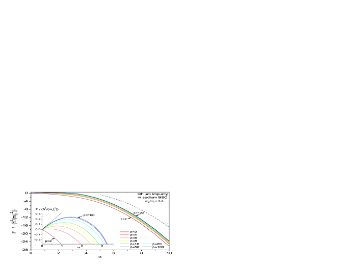
Figure 1: (Color online) The polaronic contribution (18) to the free energy of an impurity in a condensate is shown as a function of the coupling constant $\alpha$, for different values of the temperature. From top to bottom, these are $\beta=100,50,20,10,8,6,4,2$, corresponding in our example to $T=3.5,7,18,35,44,58,88$ and $175$ nK, respectively. The dashed curve shows the strong-coupling Pekar approximation. The inset zooms in on the small $\alpha$ region: the dashed line in inset shows the second order perturbation result.

IV.3 Effective mass increase

The effective polaron mass $m_{pol}$ can be derived from the path-integral propagation of a particle from $r(0)$ to a nearby point $r(\tau)=r(0)+v\tau$ by casting the resulting transition amplitude in the form $\exp\{-m_{pol}v^{2}\tau/2\}.$ Feynman notes that this procedure gives a value for $m_{pol}$ which is always within a few percent of $1+M$ with $M$ the variationally optimal mass $M$ of the trial modelFeynmanbook ; Schultz . Figure 2 shows the result for $M$ as a function of $\alpha$, for different values of the temperature. For small values of the coupling strength, the mass increases linearly with $\alpha$ as predicted by perturbation theory. However, near $\alpha\approx 3.5$, the behavior changes and the mass increases rapidly.

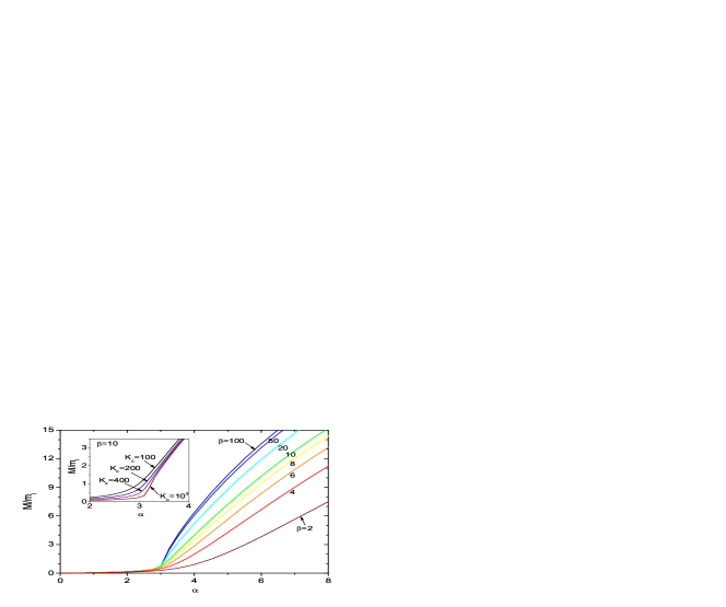
Figure 2: (Color online) The variational mass parameter $M$ is shown as a function of $\alpha.$ The effective polaron mass is to a good approximation given by $m_{pol}=m_{I}(1+M/m_{I}).$ The curves correspond to different temperatures ($\beta=100,50,20,10,8,6,4,2$, from top to bottom), at cut-off $K_{c}=200.$ The inset shows the effect of cutoff ($K_{c}=100,200,400,1000$, from top to bottom), at $\beta=10$.

The low-energy Bogoliubov excitations are sound waves, with a dispersion qualitatively similar to acoustic phonons. The effective mass of acoustic polarons – electrons interacting with acoustic phonons – shows a jump of several orders of magnitude in the effective mass (cf. acoustipol ) above a critical coupling strength. In the present case we also note a faster increase in the mass above a critical coupling strength, even though the interaction amplitude is different from that between acoustic phonons and electrons. In the dilute atomic gas, the transition is much less dramatic, and becomes smoother as temperature increases. We believe the smoothness of the crossover is not an artifact of the path-integral formalism, since in the case of the acoustic polarons it is the same formalism that predicts a discontinuous jump. For acoustic polarons, it is also predicted that the sharpness of the transition depends strongly on the cutoff: above a critical value of $K_{c}$ a discontinuity appears in the mass as a function of $\alpha$. So it is worthwhile to study the dependence of $M$ on the value of a cut-off to the $k$ integrations in (18) also in the present case. We find that increasing the cutoff sharpens the transition (as can be seen in the inset of Fig. 2), but no discontinuity arises as it does for the acoustic polaron. The difference is due to the fact that although the Bogoliubov excitation dispersion and the interaction amplitude show a similar $k$-dependence as in the case of acoustic polarons, this is only true in the limit $k\ll 1,$ and large deviations already occur for $k\approx 1$, the relevant length scale of the problem. Yet even though the transition is not as abrupt as for acoustic polarons, it is possible to distinguish two regimes. In conjunction with the crossover from positive to negative values of the free energy, this is again indicative of a transition between an quasi-free (unbound) impurity and self-trapping for the impurity.

IV.4 Polaron radius

The second variational parameter, $\Omega$, is linked to the polaron radius. Within the model system described by the action functional $\mathcal{S}_{0}$, expression (13), the expectation value of the square of the relative coordinate for the impurity – boson mass system is given by

$$\left\langle r^{2}\right\rangle=\frac{3}{2\Omega}\frac{M}{1+M}\coth\left(\frac{\beta\Omega}{2}\right)$$ (28)

The square root of this is a measure of the localization length of the impurity wave function. For strong coupling, this expectation value converges to the expectation value with respect to the variational wave function formulated by Landau and PekarPekar1946 .

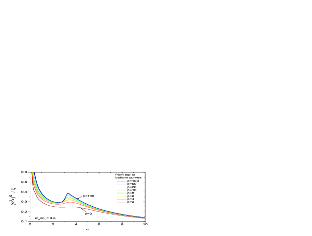
Figure 3: (Color online) The polaron radius in units of the healing length is plotted as a function of the coupling constant $\alpha$, for different temperatures. From top to bottom, $\beta=100,50,20,10,8,6,4,2$. Around $\alpha\approx 3$ nonmonotonous behavior develops as a function of $\alpha$ when the temperature is reduced.

Fig. (3) shows the polaron radius $\sqrt{\left\langle r^{2}\right\rangle}$ as a function of the coupling strength, for different values of $\beta,$ at a cut-off $K_{c}=200$. As the coupling strength is increased, the polaron radius decreases, indicating a stronger confinement of the impurity wave function. In particular the large $\alpha$ behavior might still depend on the cut-off, although a $1/\alpha$ dependence is expected independently of $K_{c}$. Near $\alpha\approx 3-3.5,$ we find that a local maximum develops and the behavior of the polaron size as a function of $\alpha$ becomes non-monotonic. It is not clear whether this local maximum is an intrinsic feature of the BEC-impurity polaron, or whether it is an artifact from the particular variational model used.

V Conclusion

When the Bogoliubov approximation applies, the Hamiltonian describing the impurity in a condensate can be cast in the form of the Fröhlich polaron Hamiltonian. The physics becomes similar to that of a Fröhlich polaron, where for the impurity in the BEC the Bogoliubov excitations have taken the role of the phonons and the interaction strength is related to the impurity-boson and boson-boson scattering lengths. The most accurate description of polaron physics in the case of electron-phonon interactions is given by Feynman’s variational treatment, which moreover allows to study the temperature dependence of observables such as the effective mass and the free energy. We have applied a Jensen-Feynman path-integral type calculation to the case of the impurity in a condensate and derived expression (18) for the free energy. Both in the free energy and the effective mass, a critical value of the coupling strength $\alpha\approx 3.5$ can be identified where the system crosses over from the weak-coupling to the strong-coupling regime. These regimes show a qualitatively different behavior of the effective mass and free energy. The sharp increase in the the effective mass in the strong-coupling regime hints at a transition from an quasi-free state to a large-mass state similar to that for acoustic polarons. It has been pointed outacoustipol that a transition from the quasi-free regime to the large-mass regime is impossible to realize in most semiconductors and III-V compounds, even in alkali halides. However, the present results indicate that it might be attainable in ultracold gases. For this purpose, we investigated the experimentally relevant values of the system parameters, and derived a useful expression (25) relating $\alpha$ to the various parameters in the case of a condensate in the Thomas-Fermi regime. This opens up the prospect to reach and investigate the strong-coupling regime in ultracold gases, whereas this regime has hitherto be inaccessible in the solid state.

- (1) I. Bloch, J. Dalibard, and W. Zwerger, Rev. Mod. Phys. 80, 885 (2008).
- (2) J. T. Devreese, A.S. Alexandrov, to appear in Reports on Progress in Physics (2009), arXiv:0904.3682.
- (3) L.D. Landau and S. I. Pekar, Zh. Eksp. Teor. Fiz. 18, 419 (1948).
- (4) H. Fröhlich, Adv. Phys. 3, 325 (1954).
- (5) R.P. Feynman, Phys. Rev. 97, 660 (1955).
- (6) E. Kartheuser, E. Evrard, and J. Devreese, Phys. Rev. Lett. 22, 94 (1969).
- (7) V.L. Gurevich, I. G. Lang, and Yu. A. Firsov, Sov. Phys. Solid St. 4, 918 (1962).
- (8) J. Devreese, J. De Sitter, and M. Goovaerts, Phys. Rev. B 5, 2367 (1972).
- (9) R. Feynman, R. Hellwarth, C. Iddings, and P. Platzman, Phys. Rev. 127, 1004 (1962).
- (10) A. S. Mishchenko, N. Nagaosa, N. V. Prokof’ev, A. Sakamoto, and B. V. Svistunov, Phys. Rev. Lett. 91, 236401 (2003).
- (11) G. De Filippis, V. Cataudella, A. S. Mishchenko, C. A. Perroni, J. T. Devreese, Phys. Rev. Lett. 96, 136405 (2006).
- (12) G.D. Mahan and J.J. Hopfield, Phys. Rev. Lett. 12, 241 (1964); V.B. Shikin and Y.P. Monarkha, Journal of Low Temp. Phys. 16, 193 (1974).
- (13) F.M. Peeters and J.T. Devreese, Phys. Rev. B 32, 3515 (1985).
- (14) A.S. Alexandrov, Phys. Rev. B 77, 094502 (2008); A.S. Alexandrov, in Polarons in Advanced Materials (Springer Series in Materials Science, vol.103, 2007), pp. 257-310, and references therein.
- (15) F. M. Cucchietti and E. Timmermans, Phys. Rev. Lett. 96, 210401 (2006).
- (16) K. Sacha and E. Timmermans, Phys. Rev. A 73, 063604 (2006).
- (17) G.D. Mahan, in Polarons in Ionic Crystals and Polar Semiconductors (ed. J. T. Devreese, North-Holland, Amsterdam, 1972), p. 553.
- (18) Jackson, S. A., and P. M. Platzman, Phys. Rev. B 24, 499 (1981); G.E. Marques, N. Studart, Phys. Rev. B 39, 4133 (1989); J. Tempere, S.N. Klimin, I.F. Silvera, J.T. Devreese, Eur. Phys. J. B 32, 329–338 (2003).
- (19) O. Penrose and L. Onsager, Phys. Rev. 104, 576 - 584 (1956).
- (20) N.N. Bogoliubov, J. Phys. (USSR) 11, 23 (1947).
- (21) L. Pitaevskii and S. Stringari, Bose-Einstein Condensation (Oxford Science Publications, Clarendon Press, Oxford, UK), 2003.
- (22) B.-B. Huang and S.-L. Wan, Chin. Phys. Lett. 26, 080302 (2009).
- (23) M. Bruderer, A. Klein, S.R. Clark, D. Jaksch, Phys. Rev. A 76, 011605 (2007).
- (24) R.P. Feynman, Statistical Mechanics: A Set Of Lectures (Addison-Wesley Publ. Co., Reading MA, USA), 1990.
- (25) H. Kleinert, Path Integrals in Quantum Mechanics, Statistics, Polymer Physics, and Financial Markets, 5th ed. (World Scientific, Singapore), 2009.
- (26) T.D. Schultz, Phys. Rev. 116, 526 (1959).
- (27) L.D. Landau and S.I. Pekar, Zh. Eksp. Teor. Fiz. 16, 341 (1946).
- (28) C. Samuelis, E. Tiesinga, T. Laue, M. Elbs, H. Knöckel, and E. Tiemann, Phys. Rev. A 63, 012710 (2000).
- (29) M. Gacesa, P. Pellegrini, and R. Côté, Phys. Rev. A 78, 010701 (2008).
- (30) S. Inouye, M. R. Andrews, J. Stenger, H.-J. Miesner, D. M. Stamper-Kurn, and W. Ketterle, Nature 392, 151 (1998).
- (31) C. A. Stan, M. W. Zwierlein, C. H. Schunck, S. M. Raupach, and W. Ketterle, Phys. Rev. Lett. 93, 143001 (2004).
- (32) A. Derevianko, W. R. Johnson, M. S. Safronova, and J. F. Babb, Phys. Rev. Lett. 82, 3589 (1999).