Quark propagator at finite temperature and finite momentum
in quenched lattice QCD

Abstract

We present an analysis of the quark spectral function above and below the critical temperature for deconfinement performed at zero and non-zero momentum in quenched lattice QCD using clover improved Wilson fermions in Landau gauge. It is found that the temporal quark correlation function in the deconfined phase near the critical temperature is well reproduced by a two-pole ansatz for the spectral function. This indicates that excitation modes of the quark field have small decay rates. The bare quark mass and momentum dependence of the spectral function is analyzed with this ansatz. In the chiral limit we find that the quark spectral function has two collective modes corresponding to the normal and plasmino excitations in the high temperature limit. Over a rather wide temperature range in the deconfined phase the pole mass of these modes at zero momentum, which corresponds to the thermal mass of the quark, is approximately proportional to temperature. With increasing bare quark masses the plasmino mode gradually disappears and the spectral function is dominated by a single pole. We also discuss quasi-particle properties of heavy quarks in the deconfined phase. In the confined phase, it is found that the pole ansatz for the spectral function fails completely.

I Introduction

The asymptotic freedom of QCD tells us that matter at extremely high temperature ($T$) becomes a simple thermodynamic system composed of weakly interacting quarks and gluons. Thermodynamic quantities approach the Stefan-Boltzmann limit for massless quarks and gluons in the high temperature limit. Deviation from this limit that arise from the temperature-dependent running gauge coupling $g$ can be calculated perturbatively BIR ; LeBellac . The excitation properties of quarks and gluons in this region can also be analyzed using perturbative techniques. The fact that $T$ dominates over all other scales allows to adopt the hard-thermal loop (HTL) approximation HTL , which enables us to calculate propagators of these fields in a gauge independent way. It is known that in leading order of HTL-resummed perturbation theory mass gaps arise in the excitation spectra of these degrees of freedom which are proportional to $gT$. They are called thermal masses LeBellac . These excitations acquire decay widths owing to medium effects, which are proportional to $g^{2}T$. At sufficiently high $T$ these widths thus are parametrically negligible compared to the thermal masses. In addition, a novel excitation, the plasmino, appears in the quark propagator, which has a minimum in its dispersion relation at nonzero momentum plasmino . Various discussions addressed the origin of such a peculiar mode Weldon:1989ys ; BBS92 ; Blaizot:1993bb ; Peshier:1999dt ; KKN06 ; Kitazawa:2007ep and its phenomenological consequences Braaten:1990wp .

As $T$ is lowered, the gauge coupling $g$ grows and perturbation theory eventually breaks down. At the same time, other scales, which are not negligible compared to $T$ emerge, and make the problem more complicated. This is, in particular, the case for the quark-gluon plasma (QGP) phase near the critical temperature of deconfinement, $T_{c}$, which is analyzed experimentally in heavy ion collision performed currently with the Relativistic Heavy Ion Collider (RHIC) RHIC . To analyze the highly non-perturbative properties of strongly interacting matter in the temperature range accessible to the RHIC experiments, a non-perturbative approach to QCD, such as lattice QCD Monte Carlo simulation, is needed.

Since the leading order HTL-resummed perturbative calculations predict that the decay widths of quarks and gluons grow faster than the thermal masses as $T$ is lowered, one may naïvely expect that for temperatures near $T_{c}$ the peaks in spectral functions of these degrees of freedom disappear. In other words, a quasi-particle description of these excitations would be inappropriate near $T_{c}$. There are, however, several arguments supporting the existence of quasi-particles with the quantum numbers of quarks in this region. For example, quasi-particles have been used successfully to describe lattice QCD results on the equation of states and susceptibilities EoS . The existence of quark quasi-particles near $T_{c}$ is also suggested by results from lattice simulations on baryon number, electric charge and strangeness fluctuations fluctuations ; newfluct . It is also notable that quark number scaling of the elliptic flow observed in the RHIC experiments Fries:2003kq suggests the existence of quark degrees of freedom in the hot and dense matter created at RHIC. Direct studies of excitation properties of quarks based on first principle lattice calculations may therefore help to clarify the physics behind these findings.

After some pioneering work on thermal properties of the quark propagator in lattice QCD simulations quark_lattice , in Karsch:2007wc the authors of the present paper investigated the spectral properties of quarks at zero momentum for two values of temperature in the deconfined phase, $T=1.5T_{c}$ and $3T_{c}$, in quenched lattice QCD in Landau gauge. In this work, we use a two-pole ansatz for the quark spectral function, $\rho(\omega,\bm{p})$, motivated by the structure of $\rho(\omega,\bm{p})$ in the high temperature limit. This ansatz includes contributions of the normal and plasmino modes and allows to analyze the importance of thermal widths of these modes. It is found that the Euclidean correlation function for quarks on the lattice is well reproduced by this ansatz. The result indicates that excitation modes of quarks form sharp peaks in $\rho(\omega,\bm{p})$ even near $T_{c}$. In this temperature range close to $T_{c}$ it also is found that the form of $\rho(\omega,\bm{p})$ is similar to that in the perturbative region. It clearly is quite different from that at $T=0$ which is given by field strength renormalization $Z(p)$ and mass function $M(p)$ T=0 .

At temperatures close to $T_{c}$, the appearance of scales which are not negligible compared to $T$ invalidates the simple picture provided by the HTL approximation, in addition to the failure of the perturbative treatment. From the analysis of simpler models, composed of fermions and bosons, it is known that the structure of $\rho(\omega,\bm{p})$ has a nontrivial dependence on the masses of fermions and bosons when these masses are comparable to $T$ BBS92 ; KKN06 ; Kitazawa:2007ep ; Harada:2008vk . Examples are the spectrum of fermions with a mass $m$ in QED or a Yukawa model with a massless boson BBS92 . In these models $\rho(\omega,\bm{p})$ is given by the HTL approximation and, in particular, receives contributions from the plasmino mode whenever $T/m$ is large enough. On the other hand, $\rho(\omega,\bm{p})$ approaches a free quark spectral function without the plasmino mode in the low temperature $T/m\to 0$ limit. As discussed in BBS92 , and summarized in Appendix A in the present paper, the numerical result, which has been obtain at the one loop order, shows that $\rho(\omega,\bm{p})$ changes continuously as a function of $T/m$ between these two limits. In Karsch:2007wc , we analyzed the dependence of $\rho(\omega,\bm{p})$ on the bare quark mass, $m_{0}$, for each $T$ and found that the lattice result are in accordance with these findings.

The main purpose of the present study is to extend the analysis of Karsch:2007wc to lower temperatures, closer to $T_{c}$, and to non-zero momentum. In addition to the temperature values analyzed before, we performed the simulations at three lower temperatures above and below $T_{c}$. We show that the results obtained in Karsch:2007wc do not change qualitatively even at $T=1.25T_{c}$. On the other hand, we find that the two-pole approximation completely fails below $T_{c}$, which indicates that excitations of quark fields with a narrow width do not exist in the confined phase. We also analyze the momentum dependence of $\rho(\omega,\bm{p})$ and show that the dispersion relations of the normal and plasmino modes behave reasonably at finite momentum. Furthermore, we discuss the spectral properties of the light and charm quarks.

An important aspect of the analysis of the quark spectral function is that these spectral functions directly reflect the symmetries of the thermal system and are sensitive to their explicit or spontaneous breaking. One can, for example, clearly observe the effect of chiral symmetry breaking in the scalar channel of the quark propagator. We show that the behavior of scalar channel is quite different between below and above $T_{c}$; while the scalar contribution to the spectral function becomes vanishingly small in the chiral limit above $T_{c}$, such a behavior is not observed below $T_{c}$. The behavior of the quark correlation function on exceptional configurations excp.conf is reported in detail in Appendix. B.

This paper is organized as follows. In the next section, we review the general properties of the quark spectral function and discuss its structure for some special cases. The setup of the numerical simulation is summarized in Sec. III. We then discuss the numerical results for the spectral function for $T>T_{c}$ in Sec. IV and Sec.V. In Sec. IV, we consider the bare quark mass dependence of the spectral function at zero momentum. This analysis is extended to finite momenta in Sec. V. Section VI is devoted to a discussion of the quark correlation function below $T_{c}$. We give a brief summary in Sec. VII. In Appendix A, we review the fermion spectral function in a Yukawa model. In Appendix B, the behavior of the quark propagator on exceptional configuration is presented.

II General properties of quark propagator and spectral function

In this section, we summarize the definition and properties of the quark propagator and the quark spectral function. While the content of this section may be familiar to many readers, this section also serves to introduce the notation used in subsequent sections. We also review the forms of the spectral function in some limiting cases which are of relevance in later sections.

II.1 Definitions

The excitation properties of quarks in a thermal medium can be extracted from the imaginary-time (Matsubara) quark propagator which is defined as,

$$S_{\mu\nu}^{bc}(\tau,\bm{x};0,\bm{y})=\langle{\rm T}_{\tau}\psi_{\mu}^{b}(\tau,\bm{x})\bar{\psi}_{\nu}^{c}(0,\bm{y})\rangle,$$ (1)

where $\tau$ is the imaginary time restricted to the interval $0\leq\tau<1/T$. Here ${\rm T}_{\tau}$ denotes the time-ordering along the imaginary time, and $\psi_{\mu}^{b}(\tau,\bm{x})$ is the quark operator, with Greek subscripts denoting the Dirac indices, and $b$ and $c$ representing colors. The thermal average $\langle{\cal O}\rangle$ is defined by $\langle{\cal O}\rangle=(1/Z){\rm Tr}[\mbox{e}^{-\beta H}{\cal O}]$, where the trace is taken over a complete set of quantum states and $Z={\rm Tr}[\mbox{e}^{-\beta H}]$. In the following analysis, we use the propagator in momentum space,

$$S_{\mu\nu}(\tau,\bm{p})=\frac{1}{VN_{c}}\sum_{b}\int d^{3}xd^{3}y\mbox{e}^{i{\bf p}\cdot({\bf x}-{\bf y})}S_{\mu\nu}^{bb}(\tau,\bm{x};0,\bm{y}),$$ (2)

where $V$ denotes the volume of the system and $N_{c}=3$ is the number of colors. Equation (2) is referred to as the correlation function in the following. Since $S_{\mu\nu}(\tau,\bm{p})$ is a gauge covariant quantity, gauge-fixing conditions are required to obtain non-zero expectation values. Equation (2) satisfies anti-periodic boundary condition along the imaginary time,

$$S_{\mu\nu}(\tau,\bm{p})=-S_{\mu\nu}(\tau-1/T,\bm{p}).$$ (3)

For zero quark chemical potential, the thermal ensemble has a charge conjugation symmetry. The thermal average thus satisfies $\langle{\cal O}\rangle=\langle{\cal COC}\rangle$, with ${\cal C}$ representing the unitary operator for charge conjugation. This symmetry leads to the following identity of the correlation function

$$S_{\mu\nu}(\tau,\bm{p}) =\left[CS^{T}(-\tau,-\bm{p})C^{-1}\right]_{\mu\nu}$$

$$=-\left[CS^{T}(1/T-\tau,-\bm{p})C^{-1}\right]_{\mu\nu},$$ (4)

where $C$ is the charge conjugation matrix; ${\cal C}\psi{\cal C}=C\psi^{T}$. In the last equality of Eq. (4), we used Eq. (3).

The Fourier transform of Eq. (2) with respect to $\tau$ is given by

$$S_{\mu\nu}(\tau,\bm{p})=T\sum_{n}\mbox{e}^{i\omega_{n}\tau}S_{\mu\nu}(i\omega_{n},\bm{p}),$$ (5)

with the Matsubara frequencies for fermions $\omega_{n}=(2n+1)\pi T$. The retarded propagator in real time is obtained by the analytic continuation of Eq. (5) as $S_{\mu\nu}^{\rm R}(\omega,\bm{p})=S_{\mu\nu}(i\omega_{n},\bm{p})|_{i\omega_{n}\to\omega+i\eta}$.

The spectral function is related to the retarded and Matsubara propagators as

$$\rho_{\mu\nu}(\omega,\bm{p}) =-(1/\pi){\rm Im}S_{\mu\nu}^{\rm R}(\omega,\bm{p})$$

$$=-(1/\pi)\left(S^{\rm R}(\omega,\bm{p})-\gamma^{0}S^{\rm R}(\omega,\bm{p})^{\dagger}\gamma^{0}\right)_{\mu\nu},$$ (6)

and

$$S_{\mu\nu}(i\omega_{n},\bm{p})=\int d\omega^{\prime}\frac{\rho_{\mu\nu}(\omega^{\prime},\bm{p})}{i\omega_{n}-\omega^{\prime}}.$$ (7)

From Eqs. (7) and (5), one obtains the relation between $\rho_{\mu\nu}(\omega,\bm{p})$ and $S_{\mu\nu}(\tau,\bm{p})$;

$$S_{\mu\nu}(\tau,\bm{p})=\int_{-\infty}^{\infty}d\omega\frac{\mbox{e}^{(1/2-\tau T)\omega/T}}{\mbox{e}^{\omega/2T}+\mbox{e}^{-\omega/2T}}\rho_{\mu\nu}(\omega,\bm{p}).$$ (8)

Using the charge conjugation symmetry, one can show that $\rho_{\mu\nu}(\omega,\bm{p})$ obeys the following relation,

$$\rho_{\mu\nu}(\omega,\bm{p})=[C\rho^{T}(-\omega,-\bm{p})C]_{\mu\nu}.$$ (9)

II.2 Dirac structure

Owing to parity and rotational symmetries, the Dirac structure of the quark spectral function at finite temperature is in general decomposed as

$$\rho_{\mu\nu}(\omega,\bm{p})$$

$$=\rho_{0}(\omega,p)(\gamma^{0})_{\mu\nu}-\rho_{\rm v}(\omega,p)(\hat{\bm{p}}\cdot\bm{\gamma})_{\mu\nu}+\rho_{\rm s}(\omega,p)\bm{1}_{\mu\nu},$$ (10)

where $p=|\bm{p}|$ and $\hat{\bm{p}}=\bm{p}/p$. Here,

$$\rho_{0}(\omega,p) ={\rm Tr}_{\rm D}[\rho(\omega,\bm{p})\gamma^{0}]/4,$$ (11)

$$\rho_{\rm v}(\omega,p) ={\rm Tr}_{\rm D}[\rho(\omega,\bm{p})\hat{\bm{p}}\cdot\bm{\gamma}]/4,$$ (12)

$$\rho_{\rm s}(\omega,p) ={\rm Tr}_{\rm D}[\rho(\omega,\bm{p})]/4,$$ (13)

with ${\rm Tr}_{\rm D}$ denoting the trace over Dirac indices. Using Eq. (9), it is shown that $\rho_{0}(\omega,p)$ is an even function and $\rho_{\rm v,s}(\omega,p)$ are odd functions of $\omega$;

$$\rho_{0}(\omega,p) =\rho_{0}(-\omega,p),$$ (14)

$$\rho_{\rm v}(\omega,p) =-\rho_{\rm v}(-\omega,p),$$ (15)

$$\rho_{\rm s}(\omega,p) =-\rho_{\rm s}(-\omega,p).$$ (16)

In some special cases, the Dirac structure of the spectral function can also be decomposed by using projection operators Blaizot:1993bb ; decomp . Two such examples, which are of relevance in the subsequent sections, are the spectral function at zero momentum and that having chiral symmetry. For the former case, $\rho_{\rm v}(\omega,p)$ vanishes and $\rho(\omega,\bm{p}=\bm{0})$ can be decomposed with the projection operators $L_{\pm}=(1\pm\gamma^{0})/2$ as

$$\rho(\omega,\bm{0})=\rho^{\rm M}_{+}(\omega)L_{+}\gamma^{0}+\rho^{\rm M}_{-}(\omega)L_{-}\gamma^{0},$$ (17)

where

$$\rho^{\rm M}_{\pm}(\omega) =\frac{1}{2}{\rm Tr}_{\rm D}[\rho(\omega,\bm{0})\gamma^{0}L_{\pm}]$$

$$=\rho_{0}(\omega,0)\pm\rho_{\rm s}(\omega,0).$$ (18)

We note that gamma matrices ($\gamma^{0}$) in Eq. (17) come directly from the definition of the quark propagator; $S(\tau)=\langle{\rm T}_{\tau}\psi(\tau)\bar{\psi}(0)\rangle=\langle{\rm T}_{\tau}\psi(\tau)\psi^{\dagger}(0)\rangle\gamma^{0}$.

If the system is chirally symmetric, the quark propagator must anti-commute with $\gamma_{5}$, and thus $\rho_{\rm s}(\omega,p)$ vanishes in Eq. (10). In this case, $\rho(\omega,\bm{p})$ can be decomposed using the projection operators $P_{\pm}(\bm{p})=(1\pm\gamma^{0}\hat{\bm{p}}\cdot\bm{\gamma})/2$ as

$$\rho(\omega,\bm{p})=\rho^{\rm P}_{+}(\omega,p)P_{+}(\bm{p})\gamma^{0}+\rho^{\rm P}_{-}(\omega,p)P_{-}(\bm{p})\gamma^{0},$$ (19)

where

$$\rho^{\rm P}_{\pm}(\omega,p) =\frac{1}{2}{\rm Tr}_{\rm D}[\rho(\omega,\bm{p})\gamma^{0}P_{\pm}(\bm{p})]$$

$$=\rho_{0}(\omega,p)\pm\rho_{\rm v}(\omega,p).$$ (20)

We note that in general $\rho^{\rm M}_{\pm}(\omega)$ and $\rho^{\rm P}_{\pm}(\omega,p)$ are neither even nor odd functions. Instead, the charge conjugation symmetry, Eq. (9), requires the following relations for $\rho^{\rm M}_{\pm}(\omega)$ and $\rho^{\rm P}_{\pm}(\omega,p)$;

$$\rho^{\rm M}_{\pm}(\omega) =\rho^{\rm M}_{\mp}(-\omega),$$ (21)

$$\rho^{\rm P}_{\pm}(\omega,p) =\rho^{\rm P}_{\mp}(-\omega,p).$$ (22)

Finally, the chirally symmetric spectral function at zero momentum is simply written as $\rho(\omega,\bm{0})=\rho_{0}(\omega,0)\gamma^{0}$. This function can be decomposed into the forms given by Eq. (17) as well as Eq. (19) with $\rho^{\rm M}_{\pm}(\omega)=\rho^{\rm P}_{\pm}(\omega,0)=\rho_{0}(\omega,0)$. Only in this case do $\rho^{\rm M}_{\pm}(\omega)$ and $\rho^{\rm P}_{\pm}(\omega,0)$ become even functions of $\omega$.

The spectral functions, $\rho^{\rm M}_{\pm}(\omega)$ and $\rho^{\rm P}_{\pm}(\omega,p)$, which arise in the decomposition of the spectral function $\rho(\omega,p)$, represent excitations having definite quantum numbers corresponding to each projection. Therefore, the excitation properties of quarks are more apparent in these channels rather than in Eqs. (11)-(13). Moreover, using the definition of the spectral function, one can prove that they are non-negative, $\rho^{\rm M}_{\pm}(\omega)\geq 0$ and $\rho^{\rm P}_{\pm}(\omega,p)\geq 0$. In the analyses presented in later sections, we therefore mainly refer to $\rho_{\pm}^{\rm M}(\omega)$ and $\rho_{\pm}^{\rm P}(\omega,0)$ instead of Eqs. (11)-(13). One can also show that $\rho_{0}(\omega,p)\geq 0$, while the signatures of $\rho_{\rm v}(\omega,p)$ and $\rho_{\rm s}(\omega,p)$ are not determined from the definition.

The correlation function $S_{\mu\nu}(\tau,\bm{p})$ is also decomposed similarly to Eq. (10),

$$S_{\mu\nu}(\tau,\bm{p})$$

$$=S_{0}(\tau,p)(\gamma^{0})_{\mu\nu}-S_{\rm v}(\tau,p)(\hat{\bm{p}}\cdot\bm{\gamma})_{\mu\nu}+S_{\rm s}(\tau,p)\bm{1}_{\mu\nu}.$$ (23)

Using the charge conjugation symmetry, one can show that $S_{0}(\tau,p)=S_{0}(1/T-\tau,p)$, $S_{\rm v,s}(\tau,p)=-S_{\rm v,s}(1/T-\tau,p)$. For zero momentum and in the chiral limit, the correlation function reduces to

$$S(\tau,\bm{0})\gamma^{0} =S^{\rm M}_{+}(\tau)L_{+}+S^{\rm M}_{-}(\tau)L_{-},$$ (24)

$$S(\tau,\bm{p})\gamma^{0} =S^{\rm P}_{+}(\tau,p)P_{+}(\bm{p})+S^{\rm P}_{-}(\tau,p)P_{-}(\bm{p}),$$ (25)

respectively. The charge conjugation symmetry requires that

$$S^{\rm M}_{\pm}(\tau)=S^{\rm M}_{\mp}(1/T-\tau),\quad S^{\rm P}_{\pm}(\tau,p)=S^{\rm P}_{\mp}(1/T-\tau,p),$$ (26)

while $S^{\rm M}_{\pm}(\tau)$ and $S^{\rm P}_{\pm}(\tau,p)$ are neither symmetric nor anti-symmetric. Only if the system is chirally symmetric, $S^{\rm M}_{+}(\tau)$ becomes a symmetric function,

$$S^{\rm M}_{+}(\tau)=S^{\rm M}_{+}(1/T-\tau).$$ (27)

II.3 Spectral functions in some special cases

II.3.1 Free quarks

The retarded propagator of a free quark with Dirac mass $m$ is given by

$$S^{\rm R}_{\rm free}(\omega,\bm{p})=\frac{1}{P/-m}=\frac{\Lambda_{+}(\bm{p};m)\gamma^{0}}{\omega+i\eta-E_{p}}+\frac{\Lambda_{-}(\bm{p};m)\gamma^{0}}{\omega+i\eta+E_{p}},$$ (28)

where $P_{\mu}=(\omega+i\eta,\bm{p})$, and $\Lambda_{\pm}(\bm{p};m)=(E_{p}\pm\gamma^{0}\bm{p}\cdot\bm{\gamma})/(2E_{p})$ are the projection operators for the free quark with $E_{p}=\sqrt{\bm{p}^{2}+m^{2}}$. The corresponding spectral function is given by $\rho(\omega,\bm{p})=\rho^{\rm free}_{+}(\omega,p)\Lambda_{+}(\bm{p};m)\gamma^{0}+\rho^{\rm free}_{-}(\omega,p)\Lambda_{-}(\bm{p};m)\gamma^{0}$ with

$$\rho^{\rm free}_{\pm}(\omega,p)=\delta(\omega\mp E_{p}).$$ (29)

The projection operators $\Lambda_{\pm}(\bm{p};m)$ satisfy $\Lambda_{\pm}(\bm{0};m)=L_{\pm}$ and $\Lambda_{\pm}(\bm{p};0)=P_{\pm}(\bm{p})$. Therefore, $\rho^{\rm M}_{\pm}(\omega)$ of the free quark with zero momentum reads

$$\rho^{\rm M}_{\pm}(\omega) =\delta(\omega\mp m),$$ (30)

and $\rho^{\rm P}_{\pm}(\omega,p)$ with zero quark mass

$$\rho^{\rm P}_{\pm}(\omega,p) =\delta(\omega\mp p).$$ (31)

II.3.2 High temperature limit

The quark propagator at asymptotically high temperature can be calculated perturbatively. The validity of HTL approximation allows to obtain gauge independent result within this approach HTL . The quark propagator at leading order in perturbation is given by

$$S^{\rm R}_{\rm HTL}(\omega,\bm{p}) =\left[P/-\Sigma_{\rm HTL}(\omega,\bm{p})\right]^{-1},$$ (32)

where

$$\Sigma_{\rm HTL}(\omega,\bm{p})$$

$$=\frac{m_{T}^{2}}{p}Q_{0}\left(\frac{\omega}{p}\right)\gamma^{0}+\frac{m_{T}^{2}}{p}\left(1-\frac{\omega}{p}Q_{0}\left(\frac{\omega}{p}\right)\right)\hat{\bm{p}}\cdot\bm{\gamma},$$ (33)

is the quark self-energy with thermal mass $m_{T}^{2}=(1/6)g^{2}T^{2}$ and $Q_{0}=(1/2)\ln(x+1)/(x-1)$ LeBellac . Since Eq. (32) is chirally symmetric, $S^{\rm R}_{\rm HTL}(\omega,\bm{p})$ and the corresponding spectral function can be decomposed using the projections operators $P_{\pm}(\bm{p})$. The spectral functions $\rho^{\rm P}_{\pm}(\omega,\bm{p})$ then read

$$\rho_{\pm}^{\rm P}(\omega,p)= Z_{\rm N}(p)\delta(\omega\mp E_{\rm N}(p))+Z_{\rm P}(p)\delta(\omega\pm E_{\rm P}(p))$$

$$+\rho_{\rm cont.}(\pm\omega,p),$$ (34)

where $\rho_{\rm cont.}(\omega,p)$ represents the contribution of the continuum taking non-zero values in the space-like region. $\rho_{+}^{\rm P}(\omega,p)$ has two poles in the time-like region at $E_{\rm N}(p)>0$ and $E_{\rm P}(p)>0$, which are called normal and (anti-)plasmino modes, respectively LeBellac . For zero momentum, $E_{\rm N}(0)=E_{\rm P}(0)=m_{T}$ and the residues satisfy $Z_{\rm N}(p)=Z_{\rm P}(p)=0.5$. The spectral functions for zero momentum thus are given by,

$$\rho_{\pm}^{\rm P}(\omega,0) =\rho_{\pm}^{\rm M}(\omega)=\rho_{0}(\omega,0)$$

$$=\frac{1}{2}\left[\delta(\omega-m_{T})+\delta(\omega+m_{T})\right].$$ (35)

II.3.3 Effect of a non-zero Dirac mass

In the derivation of Eq. (32), it is assumed that not only $g\ll 1$ but also $T$ dominates over all other scales, where the latter condition is required for the validity of the HTL approximation. If $T$ is not large enough compared to other scales, the effect of the latter shows up which leads to modifications of the form of the quark propagator even if perturbation theory is still valid. An example for such a scale is the Dirac mass of the quark, $m$. The effect of $m$ has been first investigated in BBS92 for the case of QED and for a Yukawa model composed of a massive fermion and a massless boson. In these models, the fermion spectral functions for zero momentum, $\rho^{\rm M}_{\pm}(\omega)$, take simple forms in the massless and infinite mass limits: For $m/T\to 0$, $T$ dominates over other scales and $\rho^{\rm M}_{\pm}(\omega)$ should approach Eq. (35),

$$\rho_{\pm}^{\rm M}(\omega)\simeq\frac{1}{2}\left[\delta(\omega-m_{T})+\delta(\omega+m_{T})\right].$$ (36)

However, in the opposite limit, $m/T\to\infty$, the Dirac mass dominates over $T$ and the spectral function approaches that of a free quark,

$$\rho_{\pm}^{\rm M}(\omega)\simeq\delta(\omega\mp m).$$ (37)

By comparing Eqs. (36) and (37), it is obvious that the number of poles in $\rho^{\rm M}_{\pm}(\omega)$ is different in these limits. The analysis performed in BBS92 in the one-loop approximation showed that these two limits are nevertheless connected continuously; as $m/T$ becomes smaller, the peak corresponding to the plasmino gradually manifests itself in $\rho^{\rm M}_{\pm}(\omega)$. In Appendix A, the numerical results for this feature in the Yukawa model and details of the formalism are summarized. Also in QCD, if the temperature is high enough so that the one-loop approximation for the quark self-energy is valid, we find the same limiting behavior as in Eqs. (36) and (37). At intermediate values of $m/T$ a similar behavior of $\rho^{\rm M}_{\pm}(\omega)$ as found in the model calculations is therfore also expected. Using lattice simulations, we will show in the following that the two limiting forms of the spectral function are observed even in the non-perturbative region near $T_{c}$ Karsch:2007wc in Sec. IV.

III Simulation setup

In this study, we analyze the quark correlation function, Eq. (2), using lattice QCD simulations in the quenched approximation, where vacuum excitations of the quark–anti-quark pairs are neglected. For the lattice fermion, we use non-perturbatively improved clover Wilson fermions Sheikholeslami:1985ij ; Luscher:1996jn .

We use gauge field ensembles which have been generated and used previously by the Bielefeld group to study screening masses and spectral functions Bielefeld ; Datta:2003ww . The simulation parameters are summarized in Table 1. We calculate the fermion correlation function for five values of the temperature, three of which are above $T_{c}$ and the others are below $T_{c}$. The simulation for $T>T_{c}$ is performed on lattices of three different volumina, $N_{\sigma}^{3}\times N_{\tau}$, and lattice spacing, $a$, in order to check the dependence of the numerical result on volume and lattice spacing. A column labeled $c_{\rm SW}$ in Table 1 gives the parameter for the clover coefficient. For configurations above $T_{c}$, we have checked that the average of the Polyakov loop on every configuration is closest to the $Z(3)$ root on the real axis.

To estimate the value of the lattice spacing at which our calculations for a given $T/T_{c}$ have been performed we use $T_{c}\simeq$ 300MeV. This results from determinations of $T_{c}$ in units of the square root of the string tension, $T_{c}/\sqrt{\sigma}\simeq 0.64$ Teper ; sigma ; Namekawa:2001ih and a value for the string tension, $\sqrt{\sigma}\simeq 465$ MeV, which is extracted from studies of the heavy quark potential in QCD with light quarks asqtad_pot ; our_eos . We note that the resulting estimate for the lattice cut-off has to rely on a physical scale that needs to be taken from a physical, i.e. unquenched QCD, calculation.

$T/T_{c}$	$N_{\tau}$	$N_{\sigma}$	$\beta$	$c_{\rm SW}$	$a$[fm]	$N_{\rm conf}$	$N_{\rm excp}$
$3$	$16$	$64$	$7.457$	$1.3389$	$0.014$	$51$	$0$
	$16$	$48$	$7.457$	$1.3389$	$0.014$	$51$	$0$
	$12$	$48$	$7.192$	$1.3550$	$0.019$	$51$	$0$
$1.5$	$16$	$64$	$6.872$	$1.4125$	$0.027$	$44$	$7$
	$16$	$48$	$6.872$	$1.4125$	$0.027$	$51$	$0$
	$12$	$48$	$6.640$	$1.4579$	$0.037$	$51$	$3$
$1.25$	$16$	$64$	$6.721$	$1.4404$	$0.033$	$48$	$31$
	$16$	$48$	$6.721$	$1.4404$	$0.033$	$58$	$0$
$0.93$	$16$	$48$	$6.499$	$1.4579$	$0.038$	$50$	$0$
$0.55$	$16$	$48$	$6.136$	$1.6530$	$0.075$	$60$	$1$

Table 1: Simulation parameters on lattices of size $N_{\sigma}^{3}\times N_{\tau}$. The last column labeled $N_{\rm excp}$ gives the number of exceptional configurations (see text).

Quark propagators have been calculated after fixing each gauge field configuration to Landau gauge, $\partial_{\mu}A^{\mu}=0$. For this we used conventional and stochastic minimization algorithms with a stopping criterion, $(1/3){\rm tr}|\partial_{\mu}A^{\mu}|^{2}<\alpha$ with $\alpha=10^{-11}$. By comparing the correlation functions calculated with stopping criteria $\alpha=10^{-11}$, $10^{-9}$ and $10^{-7}$, we have checked that the numerical result converges well at $\alpha=10^{-11}$.

In the Wilson fermion formulation the bare quark mass, $m$, is related to the hopping parameter $\kappa$. A naïve formula for this relation is

$$m_{0}=\frac{1}{2a}\left(\frac{1}{\kappa}-\frac{1}{\kappa_{c}}\right)\;,$$ (38)

where $\kappa_{c}$ denotes the critical hopping parameter corresponding to the chiral limit. For temperatures above $T_{c}$, we determine $\kappa_{c}$ from the $\kappa$ dependence of the quark propagator, as will be described more precisely in Sec. IV. The pole of the free Wilson fermion propagator at zero momentum, on the other hand, is given by

$$m_{p}=\frac{1}{a}\log(1+am_{0}).$$ (39)

In the following, we use Eq. (39) to define the bare quark mass, since we found that the $a$ dependence of the quark spectral function at large bare quark mass is smaller with the definition Eq. (39) rather than Eq. (38). The choice of the definitions of the bare quark mass, however, does not alter almost all discussions in this paper anyway, since our discussions never use the precise values of the bare quark mass.

For temperatures $T/T_{c}\leq 1.5$ and values of the hopping parameters close to $\kappa_{c}$ we observe on some gauge field configurations an anomalous behavior of the quark propagator. The appearance of such exceptional configurations in calculations with light quarks in quenched QCD is a well-known problem in calculations with Wilson fermions excp.conf . We discuss the behavior of the quark correlation function on these configurations in Appendix B. As summarized there, the behavior of the quark propagator on these configurations is clearly unphysical, and it is easy to introduce a reasonable criterion to distinguish them from the normal ones. The number of configurations identified to be exceptional is given in the last column of Table 1 labeled $N_{\rm excp}$. We excluded these configurations from our analysis. The number of configurations analyzed, $N_{\rm conf}$, which does not include the exceptional ones, is also given in Table 1. One sees from this table that the number of the exceptional configurations tends to increase as $T$ is lowered and as spatial volume is larger. In particular, we did not observe any exceptional configurations for $T/T_{c}=3$. On lattices for $64^{3}\times 16$ and $T=1.25T_{c}$, on the other hand, almost $40\%$ configurations are identified to be the exceptional ones. As discussed in Appendix B, this large number is attributed to a strong correlation in the appearance of exceptional configurations against the gauge update. We thus consider that the analysis with remaining $60\%$ configurations still makes sense; see Appendix B.

The quark correlation function, Eq. (1), is the inverse of the fermion matrix $K=D/-m$. To evaluate it numerically on the lattice, we solve the linear equation

$$\psi_{\rm source}=K\psi_{\rm result},$$ (40)

for a given source vector $\psi_{\rm source}$. In this study, we use a wall source with momentum $\bm{p}$

$$\psi_{\rm source}(\tau,\bm{x})=\frac{1}{V}\delta_{\tau,0}\exp(-i\bm{p}\cdot\bm{x}),$$ (41)

and construct the quark propagator, Eq. (2), from the solution of Eq. (40), $\psi_{\rm result}=K^{-1}\psi_{\rm source}$, as

$$S(\tau,\bm{p}) =\sum_{x}\mbox{e}^{i{\bf p}\cdot{\bf x}}\psi_{\rm result}(\tau,\bm{x})$$

$$=\frac{1}{V}\sum_{x,y}\mbox{e}^{i{\bf p}\cdot({\bf x-y})}S(\tau,\bm{x};0,\bm{y}),$$ (42)

where the Dirac and color indices are suppressed for simplicity. The point source $\psi_{\rm source}(\tau,\bm{x})=\delta_{\tau,0}\delta_{{\bf x},{\bf 0}}$, on the other hand, is the simplest choice for the source term, which leads to a different formula for the correlation function,

$$S(\tau,\bm{p})=\sum_{x}\mbox{e}^{i{\bf p}\cdot{\bf x}}\psi_{\rm result}(\tau,\bm{x})=\sum_{x}\mbox{e}^{i{\bf p}\cdot{\bf x}}S(\tau,\bm{x};0,\bm{0}).$$ (43)

Translational invariance requires that the two definitions for $S(\tau,\bm{p})$, Eqs. (42) and (43), should give the same result. We have confirmed that this is indeed the case within statistical error. It is, however, found that the statistical error obtained with Eq. (42) is notably smaller than that with Eq. (43) while the numerical costs are almost the same for both definitions. The advantage of the wall source becomes more prominent on lattices with larger spatial volume. This behavior is understood intuitively: In Eq. (42), the propagators of the quark field starting from various points at $\tau=0$ are averaged; this does suppress fluctuations arising from the local structure of gauge configurations.

In the subsequent sections we limit our analyses to two cases; (1) zero momentum correlators with non-zero values of the mass, $m_{p}$, and (2) finite momentum correlators in the chiral limit and above $T_{c}$. The correlation function for each case is decomposed as given in Eqs. (24) and (25), respectively. In order to reduce the statistical error of $S^{\rm M}_{+}(\tau)$ and $S^{\rm P}_{+}(\tau)$ optimally we make use of their periodicity in Euclidean time, Eq. (26), and define these correlation functions on the lattice, for example $S^{\rm M}_{+}(\tau)$, as

$$S_{+}^{\rm M}(\tau)_{\rm latt.}=\frac{1}{2}[S^{\rm M}_{+}(\tau)+S^{\rm M}_{-}(1/T-\tau)].$$ (44)

IV Quark propagator above $T_{c}$ at zero momentum

In this section, we analyze the quark spectral function above $T_{c}$ for zero momentum but with finite bare quark mass. As discussed in Sec. II, the quark spectral function at zero momentum is decomposed into $\rho^{\rm M}_{\pm}(\omega)$ as in Eq. (18). In the following, we consider $\rho^{\rm M}_{+}(\omega)$, since $\rho^{\rm M}_{-}(\omega)$ is then immediately obtained with Eq. (21).

IV.1 Lattice correlation function and fitting ansatz

In order to extract the spectral function $\rho^{\rm M}_{+}(\omega)$ from the lattice correlation function using Eq. (8) we assume a simple ansatz for the shape of $\rho^{\rm M}_{+}(\omega)$ including few fitting parameters. For the fitting function, we have tried four ansätze, two of which are single- and two-pole ones,

$$\rho^{\rm M}_{+}(\omega) =Z_{1}\delta(\omega-E_{1}),$$ (45)

$$\rho^{\rm M}_{+}(\omega) =Z_{1}\delta(\omega-E_{1})+Z_{2}\delta(\omega+E_{2}).$$ (46)

Here $Z_{1,2}$, and $E_{1,2}>0$, are fitting parameters, which represent the residues and positions of poles, respectively. The pole at $\omega=-E_{2}$ in Eq. (46) corresponds to the plasmino mode at high temperatures, while the pole at $\omega=E_{1}$ is the normal one. We have also used fitting functions that allow for a Gaussian widths,

$$\rho^{\rm M}_{+}(\omega) =\frac{Z_{1}}{\sqrt{\pi}\Gamma_{1}}\exp\frac{-(\omega-E_{1})^{2}}{\Gamma_{1}^{2}},$$ (47)

$$\rho^{\rm M}_{+}(\omega) =\frac{Z_{1}}{\sqrt{\pi}\Gamma_{1}}\exp\frac{-(\omega-E_{1})^{2}}{\Gamma_{1}^{2}}+\frac{Z_{2}}{\sqrt{\pi}\Gamma_{2}}\exp\frac{-(\omega+E_{2})^{2}}{\Gamma_{2}^{2}},$$ (48)

where $\Gamma_{1,2}$ are additional fitting parameters corresponding to the width of each peak.

Comparing the values of $\chi^{2}/{\rm dof}$ in correlated fits based on Eqs. (45) and (46), we found for all parameter sets analyzed in the present study that $\chi^{2}/{\rm dof}$ in a fit based on Eq. (46) is more than two orders of magnitude smaller than fits based on the single pole ansatz, Eq. (45). The pole corresponding to the plasmino mode at $\omega=-E_{2}$ therefore is an intrinsic feature of the quark propagator above $T_{c}$ and is needed to describe the numerical results. A single-pole ansatz Eq. (45) is clearly ruled out. Using correlated fits based on Eqs. (47) and (48), the minimal $\chi^{2}$ always is found at $\Gamma_{1}=\Gamma_{2}=0$, i.e. the ansätze reduce to Eqs. (45) and (46), respectively. The extension to include the Gaussian widths therefore does not modify the fit at all. In the following analysis, we thus use the two-pole ansatz Eq. (46).

Here, we note that the above result on the Gaussian widths is obtained in correlated fit. We checked that if we use uncorrelated fits, which neglect correlations between different $\tau$’s, the Gaussian ansätze can improve the $\chi^{2}/{\rm dof}$ especially for large bare quark masses. The numerical result shows that for large bare quark masses even the single pole ansatz with non-zero width, Eq. (47), including three parameters can give smaller $\chi^{2}/{\rm dof}$ than the four parameter fit based on Eq. (46). This shows that there exist strong correlations between different time slices on the lattice, which of course is expected.

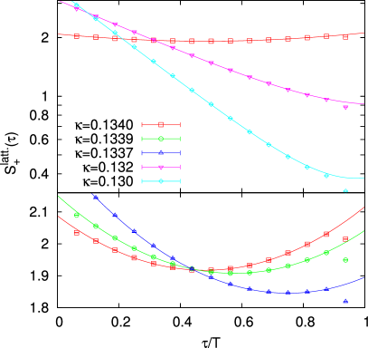
Figure 1: Lattice correlation function $S^{\rm M}_{+}(\tau)_{\rm latt.}$ at $T=3T_{c}$ for the lattice of size $64^{3}\times 16$ with various values of $\kappa$. The solid lines represent the fitting result with the two-pole ansatz, Eq. (46). Note that the upper panel shows correlation functions for the heavier quarks on a logarithmic scale and also includes the correlation function for the lightest quark mass, which also is shown again in the lower panel on a linear scale.

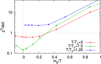
Figure 2: Bare quark mass dependence of the $\chi^{2}/{\rm dof}$ obtained for two-pole fits at $T/T_{c}=1.25$, $1.5$ and $3$ on lattices of size $64^{3}\times 16$.

In Fig. 1, we show the numerical results for $S^{\rm M}_{+}(\tau)_{\rm latt.}$ on a lattice of size $64^{3}\times 16$ at $T=3T_{c}$ for several values of $\kappa$. From the figure one sees that the shape of $S^{\rm M}_{+}(\tau)_{\rm latt.}$ approaches a single exponential function for small $\kappa$, while it becomes flat and symmetric as $\kappa$ becomes larger. In the vicinity of the source, i.e. at small and large $\tau$, we see deviations from this generic picture, which can be attributed to distortion effects arising from the presence of the source. In fact, by comparing the correlation functions on the lattices with $N_{\tau}=12$ and $16$, we find that such a distortion is clearly seen only at the $\tau$ value closest to the source. It is thus expected that this deviation arises only in the vicinity of the source and hence is negligible in the continuum limit.

In order to get control over distortion effects close to the source, we have performed fits using points $\tau_{\rm min}\leq\tau\leq N_{\tau}-\tau_{\rm min}$ with $\tau_{\rm min}=2,3,4$ and $5$ for $N_{\tau}=16$, and $\tau_{\rm min}=2,3$ and $4$ for $N_{\tau}=12$. We have checked that the dependence of the fitting parameters on $\tau_{\rm min}$ are small; the fit results obtained with different $\tau_{\rm min}$ coincide within the statistical error. In the following analysis, we use $\tau_{\rm min}=4$ and $3$ for $N_{\tau}=16$ and $12$, respectively.

The resulting correlation functions in the two-pole ansatz, Eq. (46), obtained from correlated fits are shown in Fig. 1 as solid lines. One sees that $S_{+}^{\rm M}(\tau)_{\rm latt.}$ is well reproduced by our fitting ansatz. In Fig. 2, we show the bare quark mass dependence of the $\chi^{2}/{\rm dof}$ on lattices of size $64^{3}\times 16$ and $T/T_{c}=1.25,1.5$ and $3$, where the critical hopping parameter $\kappa_{c}$ in Eq. (38) will be defined in the next subsection. The figure shows that $\chi^{2}/{\rm dof}$ is of order unity around $m_{p}=0$, which means that our fitting ansatz can describe the lattice correlation function well for light quarks. In particular, $\chi^{2}/{\rm dof}$ is less than unity for $m_{p}/T\lesssim 0.3$ with $T/T_{c}=1.5$ and $3$. For large bare quark masses and close to $T_{c}$, on the other hand, the two-pole ansatz eventually becomes worse.

The success of two-pole ansatz for the quark correlation functions indicates that the excitation modes of quarks near but above $T_{c}$ are good quasi-particles with small decay rates similar to those found in the perturbative region. In terms of the complex pole of the propagator, the results suggest that the positions of the poles would be near the real axis at $\omega=E_{1}$ and $-E_{2}$ with small imaginary parts. Provided that the positions of poles of the quark propagator are gauge independent g-dep , this also suggests that our results on the fitting parameters $E_{1}$ and $E_{2}$ have small gauge dependence.

IV.2 Pole structure

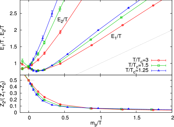
Figure 3: Bare quark mass dependence of fitting parameters $E_{1,2}$ and the relative strength of the plasmino mode, $Z_{2}/(Z_{1}+Z_{2})$, at $T/T_{c}=1.25$, $1.5$ and $3$ obtained from calculations on lattice of size $64^{3}\times 16$.

In Fig. 3, we show the dependence of $E_{1}$, $E_{2}$ and $Z_{2}/(Z_{1}+Z_{2})$ on the bare quark mass for $T/T_{c}=1.25$, $1.5$, and $3$ obtained from calculations on lattices of size $64^{3}\times 16$. Error-bars have been estimated from a Jackknife analysis. The bare quark mass $m_{p}$ is defined in Eq. (39) with $\kappa_{c}$ determined by the $\kappa$ dependence of $\rho^{\rm M}_{+}(\omega)$ as described below.

The figure shows that the ratio $Z_{2}/(Z_{1}+Z_{2})$ becomes larger with decreasing $m_{p}$ and eventually reaches $0.5$ irrespective of $T$. The numerical result for each $T$ shows that $E_{1}=E_{2}$ is satisfied within statistical errors at this point. These results show two important features of the structure of $\rho^{\rm M}_{+}(\omega)$ at this point. First, since $\rho^{\rm M}_{+}(\omega)$ becomes an even function, the quark propagator is chirally symmetric at this point within the statistical error (see Sec. II.2). Due to this feature, it is natural to define the hopping parameter satisfying $Z_{1}=Z_{2}=0.5$ to be the critical hopping parameter, $\kappa_{c}$. The values of $\kappa_{c}$ defined in this way is given in the second column of Table 2 . We have checked that these values are consistent with those obtained in Bielefeld ; Datta:2003ww from the vanishing of the isovector axial current. The second observation is that $\rho^{\rm M}_{+}(\omega)$ at $\kappa=\kappa_{c}$ has the same form as the spectral function in the high temperature limit, Eq. (35). We therefore define the thermal mass of the quark on the lattice as $m_{T}\equiv(E_{1}+E_{2})/2$ at $\kappa=\kappa_{c}$. The value of $m_{T}$ for each $T$ with $N_{\sigma}=64$ is given in the third column of Table 2. One finds that the ratio $m_{T}/T$ is insensitive to $T$ in the range analyzed in this work, although it becomes slightly larger with decreasing $T$, which would be in accordance with the expected parametric form at high temperature, $m_{T}\sim gT$.

		$m_{T}/T$
$T/T_{c}$	$\kappa_{c}$	$N_{\sigma}=64$	$N_{\sigma}=\infty$
$3$	$0.133997(13)$	$0.875(8)$	$0.771(20)$
$1.5$	$0.134999(10)$	$0.906(8)$	$0.800(18)$
$1.25$	$0.135248(10)$	$0.899(12)$	$0.803(24)$

Table 2: The second column shows the critical hopping parameter $\kappa_{c}$ determined from $\kappa$ dependence of the fitting functions for lattices of size $64^{3}\times 16$. The values of the thermal mass $m_{T}$ analyzed on lattice with $N_{\sigma}=64$, and that extrapolated to the infinite volume limit $N_{\sigma}=\infty$ are also presented in the right columns.

Figure 3 also shows that the relative strength of the plasmino pole, $Z_{2}/(Z_{1}+Z_{2})$, decreases with increasing values of the bare mass, $m_{p}$. The spectral function $\rho^{\rm M}_{+}(\omega)$ thus will eventually be dominated by a single-pole. This result agrees with the generic observations discussed in Sec. II.3, i.e. $\rho^{\rm M}_{+}(\omega)$ approaches the spectral function of free quarks, Eq. (37), as the bare quarks mass becomes larger (see also Appendix A). The quark mass dependence of the fitting parameters at large $m_{p}$ thus is reasonable. We also note that $E_{1}$ has a minimum at $m_{p}>0$, while $E_{2}$ is a monotonically increasing function. This is in contrast to the one-loop result in the Yukawa model, summarized in Appendix A, where the position of the peak in $\rho^{\rm M}_{+}(\omega)$ at positive energy corresponding to $E_{1}$ is a monotonically increasing function of $m/T$, while the absolute value of that at negative energy, $E_{2}$, decreases monotonically. The $m_{p}$ dependence of $E_{1}$ and $E_{2}$ determined from our lattice-QCD calculations therefore is qualitatively different from the perturbative result. The non-perturbative nature of the gluon field could be responsible for this behavior. Indeed, the minimum of $E_{1}$ becomes shallower with increasing temperature and the slope of $E_{2}$ decreases, as can be seen in Fig. 3. The perturbative behavior thus may well be recovered in the perturbative high temperature limit.

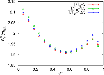
Figure 4: Lattice correlation functions near the chiral limit for $T/T_{c}=1.25$, $1.5$ and $3$. The value of $m_{p}$ is $m_{p}/T\simeq 0.1$, $0.05$ and $0.08$ for each $T$, respectively.

Finally, we shall briefly discuss the $T$ dependence of the magnitude of the residues $Z_{1}$ and $Z_{2}$. In Fig. 4 we show the correlation function $S^{\rm M}_{+}(\tau)$ near the chiral limit, $m_{p}/T\simeq 0.08$, for $T/T_{c}=1.25$, $1.5$ and $3$. The figure shows that the magnitude of $S^{\rm M}_{+}(\tau)$ is insensitive to $T$. This result indicates that the magnitude of both residues, $Z_{1}$ and $Z_{2}$, does not have a strong $T$ dependence for $T/T_{c}\gtrsim 1.25$.

IV.3 Beyond the chiral limit

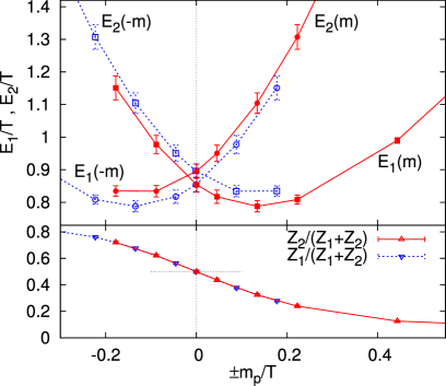
Figure 5: Fitting parameters $E_{1,2}$ and $Z_{2}/(Z_{1}+Z_{2})$ near the chiral limit for $T/T_{c}=3$. The dotted lines are $E_{1,2}$ as functions of $-m_{p}$, and $Z_{1}/(Z_{1}+Z_{2})$.

On the lattices above $T_{c}$, one can solve Eq. (40) in and even beyond the chiral limit, since chiral symmetry is not spontaneously broken above $T_{c}$ and the numerical calculation does not suffer from the light Nambu-Goldstone mode. From Eq. (39), the hopping parameter for $\kappa>\kappa_{c}$ corresponds to the negative Dirac mass. In Fig. 5, we show $m_{p}$ dependence of the fitting parameters near the chiral limit for $T/T_{c}=3$ . We plot the numerical results only for $m_{p}\gtrsim-0.2$, since the convergence of the inversion routine to solve Eq. (40) based on the BiCGStab algorithm starts failing there.

If the system possesses a charge conjugation symmetry, the sign of the Dirac mass does not affect any observables. One can, however, show that the roles of $\rho^{\rm M}_{+}(\omega)$ and $\rho^{\rm M}_{-}(\omega)$ are exchanged when the sign of the Dirac mass is reversed;

$$\rho^{\rm M}_{+}(\omega)|_{m_{p}=-m}=\rho^{\rm M}_{-}(\omega)|_{m_{p}=m}.$$ (49)

This formula is shown by the fact that $\rho_{0}(\omega,p)$ and $\rho_{\rm s}(\omega,p)$ are even and odd, respectively, as functions of the bare quark mass, and Eqs. (14) and (16). In terms of the fitting parameters in the two-pole ansatz Eq. (46), this requires that

$$E_{1}(\pm m)=E_{2}(\mp m)\mbox{ , and }Z_{1}(\pm m)=Z_{2}(\mp m).$$ (50)

In Fig. 5, $E_{1}$ and $E_{2}$ as functions of $-m_{p}$ and $Z_{1}/(Z_{1}+Z_{2})$ are shown by the dotted lines. One sees from the figure that Eq. (50) is approximately satisfied within the statistical error. This result shows that our numerical result behaves reasonably around the chiral limit. The similar result is obtained on lattices for $T=1.5T_{c}$.

IV.4 Volume and lattice spacing dependence

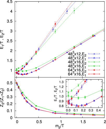
Figure 6: Bare quark mass dependence of parameters $E_{1}$, $E_{2}$, and $Z_{2}/(Z_{1}+Z_{2})$ at $T=3T_{c}$ for lattices of size $64^{3}\times 16$, $48^{3}\times 16$ and $48^{3}\times 12$.

In order to check the dependences of our results on the lattice spacing and finite volume, we analyzed the quark propagator at $T/T_{c}=3$, $1.5$ and $1.25$ on lattices with different $a$ and $N_{\sigma}$ as shown in Table 1. Results for $E_{1}$, $E_{2}$ and $Z_{2}/(Z_{1}+Z_{2})$ obtained at $T/T_{c}=3$ for two different values of the lattice cut-off and two different physical volumina are shown in Fig. 6. Comparing the results obtained on lattices with different lattice cut-off, $a$, but same physical volume, i.e. $64^{3}\times 16$ and $48^{3}\times 12$, one sees that any possible cut-off dependence is statistically not significant in our analysis. On the other hand we find a clear dependence of these quantities on the spatial volume; when comparing lattices with aspect ratios $N_{\sigma}/N_{\tau}=3$ and $4$ we find that the energy levels, $E_{1}$ and $E_{2}$, drop significantly near the chiral limit as the volume is increased. For larger values of the bare mass $m_{p}$ the volume dependence of $E_{1}$ becomes small. A similar behavior is observed for $T/T_{c}=1.5$ and $1.25$.

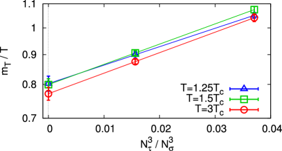
Figure 7: Extrapolation of the thermal mass of the quark to the infinite volume limit for $T/T_{c}=3$, $1.5$, and $1.25$.

The presence of a strong volume dependence of the quark propagator is not unexpected. In fact, for the emergence of the thermal mass hard gluons having momenta $p\simeq T$ play a crucial role HTL ; LeBellac . However, the lowest non-vanishing gluon momentum on the lattice is, $p_{\rm min}/T=2\pi(N_{\tau}/N_{\sigma})$, which still is larger than unity on lattices with aspect ratio $N_{\sigma}/N_{\tau}=4$. In fact, at present one cannot rule out that the discretization of low momenta can also be responsible for the success of the two-pole ansatz for $\rho_{+}^{\rm M}(\omega)$, since scattering processes giving rise to the width of quasi-particles can be suppressed due to the discretization of momentum. An analysis of quark spectral functions on lattices with even larger spatial volume, or other than periodic boundary conditions, is needed in the future to properly control effects of small momenta.

In the present study, we estimate the thermal mass $m_{T}$ in the $V\to\infty$ limit by extrapolating the results obtained for two different volumina with $N_{\tau}=16$. The extrapolation of $m_{T}$ with the ansatz for the volume dependence $m_{T}(N_{\tau}/N_{\sigma})=m_{T}(0)\exp(cN_{\tau}^{3}/N_{\sigma}^{3})$ for each temperatures is shown in Fig. 7. This extrapolation suggests that finite volume effects may still be of the order of $15\%$ in our current analysis of $m_{T}/T$. The value of $m_{T}(0)$ determined from this extrapolation is depicted in the far right columns of Table. 2.

IV.5 Quark mass dependence

$T/T_{c}$	$\kappa$	$\kappa_{c}$	$m_{D}$[GeV]	$Z_{2}/(Z_{1}+Z_{2})$
$3$	$0.13114$	$0.13454(3)$	$1.625(5)$	$0.057(2)$
$1.5$	$0.1290$	$0.13540(3)$	$1.534(6)$	$0.042(2)$

Table 3: Pole mass of the charm quark $m_{D}=E_{1}$ and the strength of the plasmino mode $Z_{2}/(Z_{1}+Z_{2})$ on $48^{3}\times 12$ lattice for $T/T_{c}=3$ and $1.5$. The parameter $\kappa$ for the charm quark is those employed in Datta:2003ww .

Here we want to discuss quasi-particle properties of the physical quarks, i.e. up, down and charm. So far we have treated the bare quark mass as a free parameter thus. Clearly one can discuss the properties at physical values of the quark masses by choosing the bare mass $m_{p}$ appropriately. Such information may be exploited for the understanding of the QGP phase near $T_{c}$.

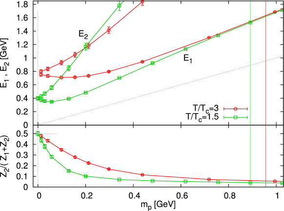
Figure 8: Dependences of $E_{1}$, $E_{2}$ and $Z_{2}/(Z_{1}+Z_{2})$ on bare quark mass $m_{p}$ on $48^{3}\times 12$ lattice for $T/T_{c}=3$ and $1.5$ in the physical unit. The value of $m_{p}$ corresponding to the charm quark employed in Datta:2003ww are shown by the vertical lines.

In order to discuss properties of the quark propagator for physical quark mass values, we first show the bare quark mass, $m_{p}$, dependences of the fitting parameters $E_{1}$, $E_{2}$ and $Z_{2}/(Z_{1}+Z_{2})$ in physical units (GeV) in Fig. 8. Throughout this subsection, we use lattices of size $48^{3}\times 12$ for $T/T_{c}=1.5$ and $3$; these sets of gauge configurations are exactly those used also in the analysis of charmonia at finite $T$ in Datta:2003ww . They are therefore most suitable for the comparison between properties of quarks and charmonia analyzed there. As discussed before, the lattice spacing dependences of these results are small and the figure hardly changes even if we employ the finer lattices of size $64^{3}\times 16$.

Let us first investigate the quasi-particle property of the charm quark. For this purpose we can use the values of $\kappa$ corresponding to the charm quark evaluated in Datta:2003ww , which are shown in Table 3. In Fig. 8, the value of $m_{p}$ corresponding to these $\kappa$ values is shown for each $T$ by a vertical line. One sees that the values of $Z_{2}/(Z_{1}+Z_{2})$ on these lines, which are shown in the far right column of Table 3, are small, $Z_{2}/(Z_{1}+Z_{2})\ll 1$. This means that the strength of the plasmino mode is weak and the structure of the quark spectral function is close to that of free quarks, Eq. (30), with a single pole at $\omega=E_{1}$. Therefore, it should be reasonable to regard the charm quarks at these temperatures as free Dirac particles with a Dirac mass $m_{D}=E_{1}$. The value of $m_{D}$ for each $T$ is shown in the fourth column of Table 3.

The lattice simulations suggest the existence of sharp peaks in the spectral function of $\eta_{c}$ and $J/\psi$ even above $T_{c}$ up to $T=1.5-2T_{c}$ charm ; Datta:2003ww . It is interesting to compare the Dirac mass of the charm quark obtained here with the spectral functions of charmonia. In particular, twice the Dirac mass, $2m_{D}$, gives a threshold for the decay process of the charmonia, provided that the potential between a quark and an antiquark vanishes at long distances. The numerical result in Datta:2003ww shows that the energies of the peaks corresponding to $\eta_{c}$ and $J/\psi$ for $T/T_{c}=1.5$ are $m_{\eta_{c}}\simeq 3.4$GeV and $m_{J/\psi}\simeq 3.8$GeV . These values are clearly larger than $2m_{D}\simeq 3.1$GeV.

If the confinement potential is screened completely, $m_{\eta_{c}}$ and $m_{J/\psi}$ thus are resonance states inside the continuum. At least at $T/T_{c}\lesssim 1.5$ the heavy quark free energy still has a complicated structure which still shows a linear rise over the distance range relevant for quarkonium physics Kaczmarek:2004gv . This needs to be taken into account in any further quantitative discussion.

Here, we note that the values of $\kappa$ employed in Datta:2003ww are not accurately corresponding to the physical charm quark: With these parameters the masses corresponding to $\eta_{c}$ in the vacuum are about $3.4$GeV and $4.1$GeV on each lattice for $T/T_{c}=1.5$ and $3$, respectively. They are therefore slightly larger than the experimental value. These parameters therefore should be interpreted as a guide for the charm quark. In particular, the values of $m_{D}$ in Table 3 are not the exact values for the charm quark. It should, however, be emphasized that the above arguments about the comparison between $2m_{D}$ and masses of charmonia makes sense, because the same hopping parameter is employed in both analyses.

Finally, we turn to a discussion on the light quarks. Figure 8 shows that the conditions $Z_{2}/(Z_{1}+Z_{2})\simeq 0.5$ and $E_{1}\simeq E_{2}$ are satisfied at $m_{p}$ corresponding to the light quark masses, say $m_{q}\simeq 0.01$GeV, for each temperature. This shows that the effect of a non-zero $m_{p}$ is negligible and the quasi-particle picture for light quarks is close to that obtained in the high-temperature limit, Eq. (35), i.e. light quarks have a thermal mass $m_{T}$. This quasi-particle property of the light quarks suggests that the effect of the thermal mass of light quarks should be taken into account when one consider quark quasi-particles as the basic ingredients in the studies of thermodynamics EoS , quarkonia and the chiral transition Hidaka:2006gd of the QGP phase near $T_{c}$. The value of the bare mass for the strange quarks, $m_{q}\simeq 0.08$ GeV, on the other hand, is in the intermediate region between the two simple limits for these temperatures.

V Quark propagator at finite momentum

In this section, we analyze the quark spectral function at finite momentum on lattices with size $64^{3}\times 16$ for $T/T_{c}=1.5$ and $3$. Throughout this section we consider the quark propagator in the chiral limit by fixing $\kappa=\kappa_{c}$, where $\kappa_{c}$ is the critical hopping parameter determined in the previous section. The correlation function on the lattice is calculated using a wall source, Eq. (42), with momentum $\bm{p}$. The quark propagator in the chiral limit is decomposed into $\rho^{\rm P}_{\pm}(\omega,p)$ according to Eq. (20). Following the same approach used in Sec. IV at zero momentum, we adopt the two-pole ansatz

$$\rho_{+}^{\rm P}(\omega,p)=Z_{1}\delta(\omega-E_{1})+Z_{2}\delta(\omega+E_{2}),$$ (51)

and determine four parameters from a correlated fit with $\tau_{\rm min}=4$. The $\delta$-functions at $\omega=E_{1}$ and $-E_{2}$ correspond to the normal and plasmino modes, respectively. We found that $\chi^{2}/{\rm dof}$ with this ansatz is always smaller than $1.5$ for all momenta analyzed in this study. This result means that the two-pole ansatz again reproduces the lattice correlation function well.

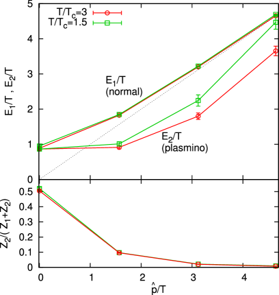
Figure 9: Dependences of the fitting parameters $E_{1}$ and $E_{2}$ and the ratio $Z_{2}/(Z_{1}+Z_{2})$ on the lattice momentum $\hat{p}=(1/a)\sin(pa)$ for $T/T_{c}=1.5$ and $3$.

In Fig. 9, we show the momentum dependence of the fitting parameters $E_{1}$, $E_{2}$, and $Z_{2}/(Z_{1}+Z_{2})$ for $T/T_{c}=1.5$ and $3$. The horizontal axis represents the momentum on the lattice $\hat{p}=(1/a)\sin pa$. The figure shows that for large momentum $Z_{2}/(Z_{1}+Z_{2})$ rapidly decreases and $E_{1}$ approaches the light cone. The spectral function at large momentum therefore approaches that of a free quark, consistent with the perturbative result. One also finds that $E_{2}$ is always smaller than $E_{1}$, in contrast to the results in Sec. IV. This behavior qualitatively agrees with the behavior of poles in the high $T$ limit LeBellac . One also observes from Fig. 9 that $E_{2}$ enters the space-like region at high momentum. While in one-loop perturbation theory the plasmino mode always exists in the time-like region, higher order corrections could give rise to such behavior of the plasmino mode. At least, such behavior does not contradict causality.

An interesting property of the quark propagator in the high temperature limit Eq. (32) is that the dispersion relation of the plasmino has a minimum at finite momentum. In Fig. 9, one sees that the value of $E_{2}$ at lowest non-zero momentum on our lattice, $p_{\rm min}=2\pi T(N_{\tau}/N_{\sigma})\simeq 1.5T$, is slightly larger than that at zero momentum, and the existence of such a minimum is suggested but not yet confirmed in the present analysis. A more detailed analysis at smaller momenta would clearly be needed, which requires calculations on lattices with a larger aspect ratio $N_{\sigma}/N_{\tau}$.

The quark spectral function at high temperatures, Eq. (34), has a continuum $\rho_{\rm cont.}(\omega,p)$ in the space-like region, which physically originates from the Landau damping. At leading order, the spectral weight of $\rho_{\rm cont.}(\omega,p)$, $\int_{-p}^{p}d\omega\rho_{\rm cont.}(\omega,p)$, becomes $0.2$ at most. The success of the two-pole fit for $\rho^{\rm P}_{+}(\omega,p)$ without the continuum therefore seems inconsistent with the perturbative result. A possible reason for this feature is the discretization of momenta on the lattice, since the Landau damping giving rise to $\rho_{\rm cont.}(\omega,p)$ can be suppressed due to the missing momenta $p\lesssim T$ in our current analysis. Lattices with much larger spatial volume are required to clarify this problem as well as the detailed properties of the dispersion relations including the minimum of the plasmino mode.

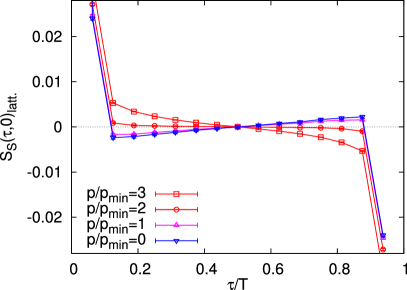
Figure 10: Scalar channel of lattice correlation function $S_{\rm s}(\tau,0)_{\rm latt.}$ at $\kappa=\kappa_{c}$ for $T/T_{c}=1.5$ with several values of $p$.

So far, we discussed the spectral functions $\rho^{\rm P}_{\pm}(\omega,p)$, assuming that the scalar channel $\rho_{\rm s}(\tau,p)$ vanishes. In order to check the validity of this assumption, we show in Fig. 10 the momentum dependence of the correlation function in the scalar channel, $S_{\rm s}(\tau,p)_{\rm latt.}$, for $T/T_{c}=1.5$. The figure shows that the absolute values of $S_{\rm s}(\tau,p)_{\rm latt.}$ are smaller than $0.005$ up to $p/p_{\rm min}\simeq 3$ except for $\tau$-values next to the source where they suffer from lattice artifacts. These values are more than two orders smaller than the typical values of $S^{\rm P}_{+}(\tau,p)_{\rm latt.}$, and thereby being negligibly small, indeed. The figure shows that deviations of $S_{\rm s}(\tau,p)_{\rm latt.}$ from zero become statistically significant as $p$ increases. This is a lattice artefact and is expected to arise from the momentum dependence of the mass term in the Wilson formulation; for free Wilson fermions the mass term is given by $M(p)=m_{0}+r(1-\cos pa)$ with $r$ being the Wilson parameter. The fact that $S_{\rm s}(\tau,p)$ is still small even at $p=3p_{\rm min}\simeq 4.5T$ shows that our lattice is fine enough so that the effect of explicit chiral symmetry breaking, which arises from the Wilson term, is well suppressed.

VI Quark propagator below $T_{c}$

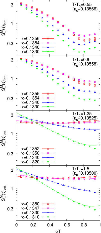
Figure 11: Lattice correlation functions $S^{\rm M}_{+}(\tau)_{\rm latt.}$ for several values of $T$ below and above $T_{c}$ on $48^{3}\times 16$ lattices. In each panel, $S^{\rm M}_{+}(\tau)_{\rm latt.}$ is depicted for four values of $\kappa$; two of which are close to $\kappa_{c}$. In the lower two panels for $T>T_{c}$, the correlation functions obtained by the two-pole ansatz is also shown by solid lines.

Next, we analyze the quark correlation function below $T_{c}$. In this section, we restrict the analysis to the lattices of size $48^{3}\times 16$ for simplicity. In the upper two panels of Fig. 11, we show the correlation function at zero momentum, $S^{\rm M}_{+}(\tau)_{\rm latt.}$, for $T/T_{c}=0.5$ and $0.93$ and for several values of $\kappa$. The critical hopping parameter $\kappa_{c}$ for each $T$ determined in Bielefeld is $0.13566$ and $0.13558$, respectively. For comparison, $S^{\rm M}_{+}(\tau)_{\rm latt.}$ above $T_{c}$ for $T/T_{c}=1.25$ and $1.5$ is shown in the lower two panels.

Before starting the discussion of results obtained below $T_{c}$, we first recapitulate the qualitative behavior of $S^{\rm M}_{+}(\tau)_{\rm latt.}$ above $T_{c}$. As we have seen in Sec. IV, the following two qualitative features are observed above $T_{c}$: (1) $S^{\rm M}_{+}(\tau)_{\rm latt.}$ is well reproduced by the two-pole ansatz Eq. (46). The fitting results are shown by solid lines in the lower two panels. (2) $S^{\rm M}_{+}(\tau)_{\rm latt.}$ approaches a symmetric function, Eq. (27), as $\kappa\to\kappa_{c}$, which means that chiral symmetry of the quark propagator is recovered there.

The upper two panels in Fig. 11 clearly show that the behavior of $S^{\rm M}_{+}(\tau)_{\rm latt.}$ below $T_{c}$ is qualitatively different from those above $T_{c}$. First, $S^{\rm M}_{+}(\tau)_{\rm latt.}$ is concave in the log-scale plot at $\tau/T\lesssim 0.6$ for any value of $\kappa$. Such structure can never be reproduced by the two-pole ansatz Eq. (46). In fact, we have checked that the fits with Eq. (46) always gives unacceptably large $\chi^{2}/{\rm dof}$ below $T_{c}$. Moreover, this behavior of $S^{\rm M}_{+}(\tau)_{\rm latt.}$ cannot be reproduced even if we use more than three poles with positive residues. Our result thus indicates the violation of positivity of $\rho^{\rm M}_{+}(\omega)$ below $T_{c}$, which is found also in the Schwinger-Dyson approach below $T_{c}$ SDE .

The failure of the two-pole ansatz for $\rho^{\rm M}_{+}(\omega)$ indicates the absence of quasi-particles corresponding to sharp peaks in $\rho^{\rm M}_{+}(\omega)$, and this result seems consistent with a naïve picture that quark excitations are confined below $T_{c}$.

In the last sections, we discussed that the gauge dependence of our result is expected to be small, due to the success of the two-pole approximation and the argument that the position of poles of propagators is gauge independent. This argument breaks down below $T_{c}$, since we no longer conclude anything about the position of poles. The violation of positivity of spectral functions could be an artifact of a specific choice of gauge fixing condition BBS92 . The calculation of $S^{\rm M}_{+}(\tau)_{\rm latt.}$ with different gauge fixing conditions may provide us with further clues to understand this problem.

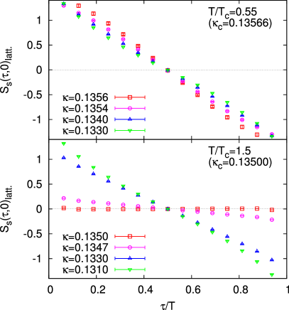
Figure 12: Scalar channel of lattice correlation function $S_{\rm s}(\tau,0)_{\rm latt.}$ for $T/T_{c}=0.5$ and $1.5$.

From Fig. 11, one also finds that $S^{\rm M}_{+}(\tau)_{\rm latt.}$ below $T_{c}$ does not approach a symmetric function as $\kappa\to\kappa_{c}$ in contrast to those above $T_{c}$. This means that the quark propagator does not become chirally symmetric even in the chiral limit, which is consistent with spontaneous chiral symmetry breaking below $T_{c}$. To see this behavior more clearly, we show in Fig. 12 the correlation function in the scalar channel, $S_{\rm s}(\tau,0)_{\rm latt.}$, for several values of $\kappa$, for $T=0.5T_{c}$ and $1.5T_{c}$. The figure shows that $S_{\rm s}(\tau,0)_{\rm latt.}$ for $T=0.5T_{c}$ indeed stays finite in the limit $\kappa\to\kappa_{c}$, while that for $T=1.5T_{c}$ is vanishingly small in this limit.

Since the difference between the correlation functions below and above $T_{c}$ is quite remarkable, we conclude that the thermal modification of gluon fields during the deconfinement transition strongly affects also the excitation properties of quarks propagating in this background field. Since our fit ansatz fails in the confined phase, however, the detailed structure of the quark propagator is less clear. The comparison with the quark propagator at $T=0$ calculated in lattice simulations T=0 and the Schwinger-Dyson equation SDE will give us insights to understand the present results. Such study, however, is beyond the scope of the present work.

VII Summary

In this publication, we analyzed the dependence of the quark spectral function on temperature $T$, bare quark mass $m$, and momentum $p$ in quenched lattice QCD with Landau gauge fixing. Above $T_{c}$, we found that the two-pole approximations for the spectral functions in the projected channels, $\rho^{\rm M}_{\pm}(\omega)$ and $\rho^{\rm P}_{\pm}(\omega,p)$, can well reproduce the lattice correlation functions. Although further studies on the volume dependence is needed, this result indicates that the excitations of quarks have small decay width even near $T_{c}$. Below $T_{c}$, on the other hand, the two-pole ansatz fails completely and the behavior of quark correlation functions indicates the violation of positivity of the spectral function.

By analyzing the $m$ and $p$ dependence of these poles, we confirmed that above $T_{c}$ two poles, the normal and plasmino excitations, appear in the quark propagator. The mass gaps of these excitation spectra should be interpreted as thermal masses, rather than Dirac mass. It is found that the ratio $m_{T}/T\simeq 0.8$ is insensitive to $T$ in the range analyzed in this study. As the bare quark mass is increased, the spectral function eventually changes its form from that having a thermal mass to the free quark form. We found that the bare quark mass of the charm quark is close to the latter, having a single mode with a Dirac mass.

All analyses of the present study are based on the quenched approximation. Although this approximation includes the leading contribution in the high temperature limit LeBellac and thus is valid at sufficiently high $T$, the validity of this approximation near $T_{c}$ is nontrivial. For example, screening of gluons due to the polarization of the vacuum with virtual quark antiquark pairs is neglected in this approximation. The coupling to possible mesonic excitations HK85 ; charm ; Datta:2003ww , which may cause interesting effects in the spectral properties of the quark KKN06 ; Kitazawa:2007ep , are not incorporated, either. The comparison of the quark propagator between quenched and full lattice QCD simulations would tell us the importance of these effects near $T_{c}$. It also would be interesting to calculate perturbatively higher order corrections to the quasi-particle properties of quarks Harada:2008vk . Such a calculation will help to clarify the origin of differences in the mass and momentum dependence of the quark propagator found in our lattice calculation in comparison to leading order perturbation theory.

There are many open questions that need to be analyzed in more detail in future calculations. A numerical simulation with a large spatial volume is an important subject among them. As discussed in the text, the influence of momenta smaller than the temperature is not properly included in the present simulations; the smallest non-zero momentum possible on our lattices with aspect ratio 4 and periodic boundary conditions is larger than $T$. Lattices allowing for momenta less than $T$ will be necessary to systematically analyze the importance of low momentum excitations. The existence of a minimum in the plasmino mode could also be confirmed in such a study. The calculation of the quark propagator in a different gauge is also important. It will allow to check directly the gauge dependence of the present results. These subjects will be studied elsewhere.

Appendix A Quark spectral function in Yukawa model

In this appendix, we review the spectral function of massive fermions coupled to a massless scalar boson via the Yukawa coupling at finite temperature $T$. While the results given in this appendix are essentially the same as those first discussed in BBS92 , we recapitulate them to make this paper self-contained. The details of the analysis in the Yukawa models at finite $T$ are found, for example, in BBS92 and KKN06 ; Kitazawa:2007ep .

We start from the Lagrangian of a Yukawa model,

$${\cal L}=\bar{\psi}(i\partial/-m)\psi+\frac{1}{2}\partial_{\mu}\phi\partial^{\mu}\phi-g_{\rm y}\phi\bar{\psi}\psi,$$ (52)

where $\psi$ and $\phi$ denote the fermion and boson operators, $m$ is the fermion mass, and $g_{\rm y}$ represents the Yukawa coupling. We neglect the mass term of the scalar boson, since the purpose of this analysis is a study of quarks coupled to massless gauge bosons. It is argued in BBS92 that the qualitative result about the fermion spectral function hardly changes even if we promote the scalar field in Eq. (52) to the $U(1)$ gauge field. In the following, we call the fermion field $\psi$ the quark.

The quark self-energy in the imaginary-time formalism at one-loop order is given by,

$$\tilde{\Sigma}(i\omega_{m},\bm{p})$$

$$=-g_{\rm y}^{2}T\sum_{n}\int\frac{d^{3}k}{(2\pi)^{3}}{\cal S}_{0}(i\omega_{n},\bm{k}){\cal D}_{0}(i\omega_{m}-i\omega_{n},\bm{p}-\bm{k}),$$ (53)

where ${\cal S}_{0}(i\omega_{n},\bm{p})=[i\omega_{n}\gamma^{0}-\bm{p}\cdot\bm{\gamma}-m]^{-1}$ and ${\cal D}_{0}(i\nu_{n},\bm{p})=[(i\nu_{n})^{2}-\bm{p}^{2}]^{-1}$ are the Matsubara propagators for the free quark and the free scalar boson, respectively, with $\omega_{n}=(2n+1)\pi T$ and $\nu_{n}=2n\pi T$. After summation over $n$ and analytic continuation, one obtains the self-energy in the real time, $\Sigma(\omega,\bm{p})=\tilde{\Sigma}(i\omega_{n},\bm{p})|_{i\omega_{n}\to\omega}$.

The self-energy $\Sigma(\omega,\bm{p})$ has an ultraviolet divergence, which can be removed with a standard renormalization BBS92 ; KKN06 ; Kitazawa:2007ep . Here we simply neglect the $T$-independent part, $\Sigma_{T=0}(\omega,\bm{p})\equiv\lim_{T\to 0}\Sigma(\omega,\bm{p})$, which includes the divergence. This approximation is justified if the temperature is high enough, since the $T$-dependent part, $\Sigma_{T\neq 0}(\omega,\bm{p})\equiv\Sigma(\omega,\bm{p})-\Sigma_{T=0}(\omega,\bm{p})$, grows rapidly and dominates over $\Sigma_{T=0}(\omega,\bm{p})$ as $T$ is raised. The $T$-dependent part $\Sigma_{T\neq 0}(\omega,\bm{p})$ does not suffer from any divergences and can be calculated without renormalization. The spectral function at one-loop order is then given by,

$$\rho(\omega,\bm{p})=-\frac{1}{\pi}{\rm Im}\frac{1}{(\omega+i\eta)\gamma^{0}-\bm{p}\cdot\bm{\gamma}-m-\Sigma(\omega,\bm{p})}.$$ (54)

In our formalism, $m$ and $T$ are the only dimensionfull parameters and thus they control all properties of the system with a fixed Yukawa coupling $g_{\rm y}$. In particular, the dimensionless spectral function, $\tilde{\rho}=T\rho(\omega/T,\bm{p}/T)$, is determined uniquely for a given ratio $T/m$. The limit $T/m\to 0$ corresponds to low temperature, where $\rho(\omega,\bm{p})$ approaches the spectral function of free quarks, Eq. (29). The opposite limit, $T/m\to\infty$, represents the high temperature limit. If we take $g_{\rm y}\to 0$ in this limit, $\rho(\omega,\bm{p})$ becomes that calculated in the HTL approximation Eq. (34) with $m_{T}=g_{\rm y}T/4$. With a fixed nonzero $g_{\rm y}$, the $\delta$-functions in $\rho(\omega,\bm{p})$ become peaks having a non-zero width of order $g_{\rm y}^{2}T$. One can, however, check numerically that the qualitative structure of $\rho(\omega,\bm{p})$ hardly changes with a small Yukawa coupling $g_{\rm y}\lesssim 1$.

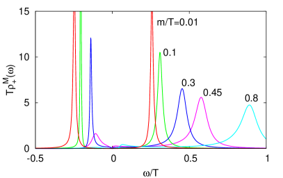
Figure 13: Spectral function $\rho^{\rm M}_{+}(\omega)$ in the Yukawa model Eq. (52) for several values of $m/T$ with a Yukawa coupling $g_{\rm y}=1$.

To compare the spectral function in the Yukawa model with the results in Sec. IV, we limit our attention to zero momentum. In this case, $\rho(\omega,\bm{0})$ is decomposed as in Eq. (17) with projection operators $L_{\pm}$. In the following we also regard $m/T$ as the external parameter, instead of $T/m$, since this is much more convenient for the comparison with the lattice result. From the above argument, one expects that the spectral function $\rho^{\rm M}_{+}(\omega)$ in the limit $m/T\to\infty$ approaches the free quark form, Eq. (30),

$$\lim_{m/T\to\infty}\rho^{\rm M}_{+}(\omega)\simeq\delta(\omega-m),$$ (55)

while in the opposite limit $m/T\to 0$, $\rho^{\rm M}_{+}(\omega)$ should approach Eq. (35),

$$\lim_{m/T\to 0}\rho^{\rm M}_{+}(\omega)\simeq\frac{1}{2}\left(\delta(\omega-m_{T})+\delta(\omega+m_{T})\right).$$ (56)

We show the numerical result for $\rho^{\rm M}_{+}(\omega)$ for several values of $m/T$ in Fig. 13. A fixed Yukawa coupling $g_{\rm y}=1$ is employed in this calculation: We have checked that the qualitative feature of the numerical result does not change with a variation of $g_{\rm y}$ over a rather wide range. The figure shows that $\rho^{\rm M}_{+}(\omega)$ for $m/T=0.01$ qualitatively reproduces Eq. (56), having two peaks around $\omega=\pm gT/4$. As $m/T$ increases, the peak at negative energy corresponding to the plasmino ceases to exist, and $\rho^{\rm M}_{+}(\omega)$ is eventually dominated by a single peak at positive energy $\omega\simeq m$. Although in the figure the width of the peak at positive energy, $\Gamma$, grows as $m/T$ increases, one can check numerically and analytically that $\Gamma/m$ vanishes in the limit $m/T\to\infty$. The width of the peak therefore is negligible in this limit, and $\rho^{\rm M}_{+}(\omega)$ reproduces Eq. (55).

The numerical result presented in Fig. 13 shows that the two limits given by Eqs. (55) and (56), respectively, are connected continuously at the one-loop order. It is also seen that the absolute value of the position of the peak at positive (negative) energy is a monotonically increasing (decreasing) function of $m/T$. As discussed in the text, this feature is qualitatively different from that observed on the lattice near but above $T_{c}$.

Appendix B Exceptional configurations

As mentioned in Sec. III, we found that the quark correlation functions $S(\tau,\bm{p})$ on some gauge configurations for $T/T_{c}\leq 1.5$ behave anomalously near the chiral limit and at zero momentum. In this appendix, we summarize the behavior of $S(\tau,\bm{p})$ on such exceptional configurations (EC). A criterion to determine the EC used in the present analysis is also described.

Figure 14: Quark correlation functions in the vector, scalar, pseudo-scalar and tensor channels, $S_{\rm V,0}(\tau)$, $S_{\rm S}(\tau)$, $S_{\rm P}(\tau)$ and $S_{\rm T,12}(\tau)$ (from top to bottom) on all configuration for a lattice of size $64^{3}\times 16$ for $T/T_{c}=1.5$. The exceptional configurations are shown by the bold lines.

For the moment, we consider the correlation function at zero momentum in the chiral limit $\kappa=\kappa_{c}$ on the lattice of size $64^{3}\times 16$ for $T/T_{c}=1.5$ ($\beta=6.872$). The Dirac structure of $S(\tau,\bm{0})$ is decomposed as

$$S_{\rm S}(\tau) ={\rm Tr}_{\rm D}\left[S(\tau,\bm{0})\right]/4,$$ (57)

$$S_{\rm V,\mu}(\tau) ={\rm Tr}_{\rm D}\left[\gamma_{\mu}S(\tau,\bm{0})\right]/4,$$ (58)

$$S_{\rm T,\mu\nu}(\tau) ={\rm Tr}_{\rm D}\left[\sigma_{\mu\nu}S(\tau,\bm{0})\right]/4,$$ (59)

$$S_{\rm A,\mu}(\tau) ={\rm Tr}_{\rm D}\left[\gamma_{\mu}\gamma_{5}S(\tau,\bm{0})\right]/4,$$ (60)

$$S_{\rm P}(\tau) ={\rm Tr}_{\rm D}\left[\gamma_{5}S(\tau,\bm{0})\right]/4.$$ (61)

In Fig. 14, we show $S_{\rm V,0}(\tau)$, $S_{\rm S}(\tau)$, $S_{\rm P}(\tau)$, and $S_{\rm T,12}(\tau)$ on all $51$ configurations. Among them, seven configurations are specified as the EC which are depicted by the bold lines. The numbers $1$-$7$ are also assigned to these lines for better identification of each configuration. The correlation functions obtained on the other $44$ configurations are shown by thin light-blue lines, which are, however, almost degenerated in the lower three panels. From the figure, one clearly sees that the behavior of $S_{\rm S}(\tau)$, $S_{\rm P}(\tau)$, and $S_{\rm T,12}(\tau)$ on the EC is qualitatively different from other normal configurations which are approximately zero in these channels. As discussed in Sec. II, the chiral, parity, and rotational symmetries require that the correlation functions in these channels vanish. The behavior of these functions on the EC therefore is obviously unphysical. On the other hand, $S_{\rm V,0}(\tau)$ tends to behave moderately even on the EC.

Figure 15: Values of $\Delta_{\rm P}$ and $\Delta_{\rm T,12}$ on all configurations for a lattice of size $64^{3}\times 16$ and $T/T_{c}=1.5$.

Since the anomalous behavior of $S_{\rm S}(\tau)$, $S_{\rm P}(\tau)$, and $S_{\rm T,12}(\tau)$ on the EC is quite evident, it is easy to introduce a criterion to identify the EC. Here, we introduce

$$\Delta_{\Gamma}=\sum_{\tau=\tau_{\rm min}}^{N_{\tau}-\tau_{\rm min}}|S_{\Gamma}(\tau)|^{2},$$ (62)

for each configuration where $\Gamma$ defines different channels Eqs. (57) - (61), and regard the configurations satisfying

$$\Delta_{\Gamma}>D,$$ (63)

as the exceptional ones with $D$ being the threshold to be determined empirically. We show $\Delta_{\rm P}$ and $\Delta_{\rm T,12}$ with $\tau_{\rm min}=3$ on all configurations in Fig. 15. The horizontal axis represents the different gauge configurations which are ordered according to Monte Carlo time. One sees that $\Delta_{\rm P}$ and $\Delta_{\rm T,12}$ on the EC take values more than two orders of magnitude larger than the typical ones on the normal configurations. This result means that there is a wide range for the choice of $D$ in Eq. (63), and hence this criterion works well in practice. Our numerical result shows that the criterion Eq. (63) is most successfully applied to the pseudoscalar channel, $\Delta_{\rm P}$, and successively $\Delta_{{\rm T},ij}$ with $1\leq i,j\leq 3$. Here, we notice that our formula for $S(\tau,\bm{p})$ with the wall source Eq. (42), instead of Eq. (43), plays a crucial role for this clear separation between the normal and exceptional configurations. In fact, with the correlation function calculated with Eq. (43), the quark correlation functions have large fluctuations and the range of $D$ which separates the EC with Eq. (63) becomes narrower.

Figure 16: Behavior of the correlation functions $S_{\rm RL}(\tau)$ on all configurations for a lattice of size $64^{3}\times 16$ and $T/T_{c}=1.5$. The exceptional configurations are shown by the bold lines.

Figure 15 also shows that the EC on this set of gauge configurations are strongly correlated. They correspond to subsequent configurations in Monte Carlo time, although the separation between these gauge configurations is a few times larger than the autocorrelation length measured in terms of the plaquette and Polyakov loop correlation functions Bielefeld . This shows that the correlation among EC is significantly stronger and leads to a much larger autocorrelation length. A similar result is obtained for $T/T_{c}=1.25$, although in this case we observed several groups of such successive EC.

Next, in Fig. 16 we show the correlation function representing the propagation between right and left handed quarks, $\psi_{\rm R,L}=(1/2)(1\pm\gamma_{5})\psi$,

$$S_{\rm RL}(\tau) =\langle{\rm T}_{\tau}\psi_{\rm R}(\tau)\bar{\psi}_{\rm L}(0)\rangle={\rm Tr}_{\rm D}[\frac{1+\gamma_{5}}{2}S(\tau,\bm{0})]$$

$$=\frac{1}{2}(S_{\rm S}(\tau)+S_{\rm P}(\tau)).$$ (64)

The figure shows that $S_{\rm RL}(\tau)$ is close to zero as it should be even on the EC. On the other hand, the opposite channel $S_{\rm LR}(\tau)={\rm Tr}_{\rm D}[S(\tau,\bm{0})(1-\gamma_{5})/2]=(S_{\rm S}(\tau)-S_{\rm P}(\tau))/2$ behaves anomalously on the EC, as expected from the behavior of $S_{\rm S,P}(\tau)$ in Fig. 14. Although on the gauge configurations for $T/T_{c}=1.5$ we observed the anomalous behavior only on $S_{\rm LR}(\tau)$ for all configurations, we checked that for $T/T_{c}=1.25$ there appear anomalous behaviors in both $S_{\rm LR}(\tau)$ and $S_{\rm RL}(\tau)$. For $T/T_{c}=1.25$, however, only one of them tends to behave anomalously on each EC with a few exceptions. It is also found that the channel having the exceptional behavior tends to be common in a group of configurations appearing successively. The results presented above indicate that there exist topological objects on the EC that cause the anomalous behavior of the quark correlation functions. To check this speculation, it would be interesting to directly measure the topological charge on each configuration.

Finally, we remark on a relation between EC observed in the quark correlation function and those in the hadronic channels. By measuring the pion correlation function constructed from the quark correlation function with the point source, Eq. (43), we confirmed that the appearance of anomalous behavior in the pion correlation function is limited on the EC determined with the criterion Eq. (63). We, however, also found that the behavior of pion propagator seems moderate on some configurations satisfying Eq. (63). The latter behavior may be attributed to the form of the lattice correlation function: As mentioned above, the wall source, Eq. (42), for the quark propagator drastically reduces the statistical fluctuations compared to the point source, and hence allows the clear separation of EC with a criterion like Eq. (63). For the same reason, the fluctuations in the pion channel can be large when calculated with a point source and such fluctuations make the identification of the EC difficult. We thus expect that if we would calculate the pion correlation function with a wall source operator similar to that used in Eq. (42) for the quarks, there would be a perfect correspondence in the appearance of the exceptional behavior in both correlation functions.

References

- (1) J. P. Blaizot, E. Iancu and A. Rebhan, Phys. Lett. B 470, 181 (1999) [arXiv:hep-ph/9910309]; Phys. Rev. D 63, 065003 (2001) [arXiv:hep-ph/0005003]; hep-ph/0303185, and references therein.
- (2) M. Le Bellac, Thermal Field Theory (Cambridge University Press, Cambridge, England 1996).
- (3) R. D. Pisarski, Phys. Rev. Lett. 63, 1129 (1989); E. Braaten and R. D. Pisarski, Nucl. Phys. B 337, 569 (1990); ibid., B339, 310 (1990).
- (4) V.V. Klimov, Sov. J. Nucl. Phys. 33, 934 (1981) [Yad. Fiz. 33, 1734 (1981)]; H.A. Weldon, Phys. Rev. D 28, 2007 (1983).
- (5) H. A. Weldon, Phys. Rev. D 40, 2410 (1989).
- (6) G. Baym, J. P. Blaizot and B. Svetitsky, Phys. Rev. D 46, 4043 (1992).
- (7) J. P. Blaizot and J. Y. Ollitrault, Phys. Rev. D 48, 1390 (1993) [arXiv:hep-th/9303070].
- (8) A. Peshier and M. H. Thoma, Phys. Rev. Lett. 84, 841 (2000) [arXiv:hep-ph/9907268].
- (9) M. Kitazawa, T. Kunihiro and Y. Nemoto, Phys. Lett. B 633, 269 (2006) [arXiv:hep-ph/0510167]; Prog. Theor. Phys. 117, 103 (2007) [arXiv:hep-ph/0609164].
- (10) M. Kitazawa, T. Kunihiro, K. Mitsutani and Y. Nemoto, Phys. Rev. D 77, 045034 (2008) [arXiv:0710.5809 [hep-ph]].
- (11) E. Braaten, R. D. Pisarski and T. C. Yuan, Phys. Rev. Lett. 64, 2242 (1990).
- (12) I. Arsene et al., Nucl. Phys. A 757, 1 (2005) [arXiv:nucl-ex/0410020]; B. B. Back et al., ibid. 757, 28 (2005) [arXiv:nucl-ex/0410022]; J. Adams et al., ibid. 757, 102 (2005) [arXiv:nucl-ex/0501009]; K. Adcox et al., ibid. 757, 184 (2005) [arXiv:nucl-ex/0410003].
- (13) M. Bluhm, et al., Phys. Rev. C 76, 034901 (2007) [arXiv:0705.0397 [hep-ph]]; M. Bluhm and B. Kampfer, Phys. Rev. D 77, 114016 (2008) [arXiv:0801.4147 [hep-ph]].
- (14) R. V. Gavai and S. Gupta, Phys. Rev. D 73, 014004 (2006) [arXiv:hep-lat/0510044]; S. Ejiri, F. Karsch and K. Redlich, Phys. Lett. B 633, 275 (2006) [arXiv:hep-ph/0509051].
- (15) M. Cheng et al., Phys. Rev. D 79, 074505 (2009).
- (16) R. J. Fries, B. Muller, C. Nonaka and S. A. Bass, Phys. Rev. C 68, 044902 (2003) [arXiv:nucl-th/0306027].
- (17) G. Boyd, F. Karsch and S. Gupta, Nucl. Phys. B 385 (1992) 481; P. Petreczky et al., Nucl. Phys. Proc. Suppl. 106 (2002) 513; M. Hamada et al., arXiv:hep-lat/0610010.
- (18) F. Karsch and M. Kitazawa, Phys. Lett. B 658, 45 (2007) [arXiv:0708.0299 [hep-lat]].
- (19) P. O. Bowman, et al., Lect. Notes Phys. 663, 17 (2005), and references therein; P. O. Bowman, U. M. Heller and A. G. Williams, Phys. Rev. D 66, 014505 (2002) [arXiv:hep-lat/0203001]; M. S. Bhagwat, M. A. Pichowsky, C. D. Roberts and P. C. Tandy, Phys. Rev. C 68, 015203 (2003) [arXiv:nucl-th/0304003]; S. Furui and H. Nakajima, Phys. Rev. D 73, 074503 (2006).
- (20) M. Harada and Y. Nemoto, Phys. Rev. D 78, 014004 (2008) [arXiv:0803.3257 [hep-ph]]; M. Harada and S. Yoshimoto, arXiv:0903.5495 [hep-ph].
- (21) W. A. Bardeen et al., Phys. Rev. D 57, 1633 (1998) [arXiv:hep-lat/9705008]; T. A. DeGrand, A. Hasenfratz and T. G. Kovacs, Nucl. Phys. B 547, 259 (1999) [arXiv:hep-lat/9810061].
- (22) H. A. Weldon, Phys. Rev. D 61, 036003 (2000) [arXiv:hep-ph/9908204].
- (23) B. Sheikholeslami and R. Wohlert, Nucl. Phys. B 259, 572 (1985).
- (24) M. Luscher, S. Sint, R. Sommer and H. Wittig, Nucl. Phys. B 491, 344 (1997) [arXiv:hep-lat/9611015].
- (25) F. Karsch et al., Phys. Lett. B 530, 147 (2002) [arXiv:hep-lat/0110208]; see also Sönke Wissel, Ph.D thesis, Bielefeld University, 2006.
- (26) S. Datta, F. Karsch, P. Petreczky and I. Wetzorke, Phys. Rev. D 69, 094507 (2004) [arXiv:hep-lat/0312037].
- (27) B. Lucini, M. Teper and U. Wenger, JHEP 0502, 033 (2005)
- (28) B. Beinlich, F. Karsch, E. Laermann and A. Peikert, Eur. Phys. J. C 6, 133 (1999) [arXiv:hep-lat/9707023].
- (29) Y. Namekawa et al. [CP-PACS Collaboration], Phys. Rev. D 64, 074507 (2001) [arXiv:hep-lat/0105012].
- (30) C. Aubin et al., Phys. Rev. D 70, 094505 (2004).
- (31) M. Cheng et al., Phys. Rev. D 77, 014511 (2008).
- (32) A. K. Rebhan, Phys. Rev. D 48, 3967 (1993).
- (33) M. Asakawa and T. Hatsuda, Phys. Rev. Lett. 92, 012001 (2004) [arXiv:hep-lat/0308034]; T. Umeda, K. Nomura and H. Matsufuru, Eur. Phys. J. C 39S1, 9 (2005) [arXiv:hep-lat/0211003]; G. Aarts, et al., Phys. Rev. D 76, 094513 (2007) [arXiv:0705.2198 [hep-lat]].
- (34) O. Kaczmarek, F. Karsch, F. Zantow and P. Petreczky, Phys. Rev. D 70, 074505 (2004) [Erratum-ibid. D 72, 059903 (2005)] [arXiv:hep-lat/0406036].
- (35) Y. Hidaka and M. Kitazawa, Phys. Rev. D 75, 011901 (2007) [Erratum-ibid. D 75, 099901 (2007)] [arXiv:hep-ph/0610374].
- (36) C. D. Roberts and S. M. Schmidt, Prog. Part. Nucl. Phys. 45, S1 (2000) [arXiv:nucl-th/0005064]; R. Alkofer, W. Detmold, C. S. Fischer and P. Maris, Phys. Rev. D 70, 014014 (2004) [arXiv:hep-ph/0309077].
- (37) T. Hatsuda and T. Kunihiro, Phys. Rev. Lett. 55, 158 (1985).