Temporal precision of spike response to fluctuating input in pulse-coupled networks of oscillating neurons

Abstract

A single neuron is known to generate almost identical spike trains when the same fluctuating input is repeatedly applied. Here, we study the reliability of spike firing in a pulse-coupled network of oscillator neurons receiving fluctuating inputs. We can study the precise responses of the network as synchronization between uncoupled copies of the network by a common noisy input. To study the noise-induced synchronization between networks, we derive a self-consistent equation for the distribution of spike-time differences between the networks. Solving this equation, we elucidate how the spike precision changes as a function of the coupling strength.

Reliable information processing requires a code that can be represented and transmitted reliably within the precision of the devices. In the brain, single neurons can generate highly precise spike trains when they are repeatedly activated by the same fluctuating inputbryant . Neurons, however, work collectively rather than individually in their network. It remains unclear whether precise elements put in a network can still respond precisely since mutual couplings may affect the response of the individual neuronstiesinga08 . To answer this question, we investigate the temporal precision of responses of a pulse-coupled network of oscillators when a set of independent fluctuating inputs, i.e., frozen noise, is repeatedly applied to the network. To study this problem analytically, we introduce uncoupled copies of the network that commonly receive the set of fluctuating inputs. Suppose that the original network repeatedly generates identical precisely-timed spike responses. Then, we can interpret the collection of these responses across trials as responses of the individual copies in a trial. Thus, in-phase synchronization between identical networks implies precisely-timed responses of a single network across trials.

Such noise-induced synchronization was previously studied between single oscillatorsteramae ; piko ; nakao . Here, we study the noise-induced synchronization between networks of oscillators to clarify whether each network is able to encode information about fluctuating inputs into precisely-timed spikes. Noise-induced synchronization can appear in laserslaser , chemical reactionschemical , gene networksgene , electronic circuits and neural systems. For instance, noise-induced synchronization of neural oscillators may play an active role in olfactory information processinggalan . An attempt was made to employ such an oscillating synchronization for a dynamic clock in digital VLSI devicesutagawa . Thus, clarifying the underlying mechanism has significant implications for a variety of dynamical systems.

We develop a mean-field theory of noise-induced synchronization between the copies of the pulse-coupled oscillator network. We can analytically derive a self-consistent equation for the distribution of phase differences between the corresponding oscillators and obtain the distribution as a function of the coupling strength. In so doing, we assume that the average of the connections projecting to each oscillator vanishes. The distribution allows us to reveal the nontrivial effect of mutual couplings on the noise-induced synchronization of oscillator networks or, equivalently, the temporal precision of responses in an oscillator network.

Let us consider multiple trials in which a pulse-coupled network of homogeneous $N$ oscillating neurons receive the same fluctuating input in all trials:

$$\dot{\bm{x}}_{i}^{\left(\alpha\right)}=\bm{F}\left(\bm{x}_{i}^{\left(\alpha\right)}\right)+\sum_{j=1}^{N}g_{ij}\sum_{n}\delta\left(t-t_{j,n}^{\left(\alpha\right)}\right)+\xi_{i}\left(t\right),$$ (1)

where $i=1,\cdots,N$, $\bm{x}_{i}^{\left(\alpha\right)}$ is the state variable of the $i$th neuron in the $\alpha$th trial, $\bm{F}\left(\bm{x}_{i}^{\left(\alpha\right)}\right)$is the intrinsic dynamics of the neuron, $g_{ij}$ is the coupling strength from the $j$th to the $i$th neuron, $t_{j,n}^{\left(\alpha\right)}$ is the $n$th spike time of the $j$th neuron in the $\alpha$th trial, and $\xi_{i}\left(t\right)$ is the fluctuating input to the $i$th neuron. $\bm{F}\left(\bm{x}\right)$ has a stable limit-cycle solution $\bm{x}_{0}\left(t\right)$ satisfying $\dot{\bm{x}_{0}}=\bm{F}\left(\bm{x}_{0}\right)$ with period $T$. Isolated neurons thus fire regularly with a firing rate $r=1/T$. We use the zero mean white Gaussian noise with variance $D$ as the fluctuating input $\xi_{i}\left(t\right)$, which is independent among neurons whereas it should be the same across trials, $\left<\xi_{i}(t)\right>=0$, $\left<\xi_{i}(t)\xi_{j}(s)\right>=D\delta_{ij}\delta(t-s)$. Since Eq. (1) is a stochastic differential equation, we have to clarify its interpretation. We use the Stratonovich interpretation, namely, we define the white noise as the limit of colored noise with infinitesimal correlation timestrato . Components of the zero mean matrix $g_{ij}$ take both positive and negative values independently, while they should also be exactly the same across trials. We denote the variance of the matrix as $G$, $\left<g_{ij}\right>=0$, $\left<g_{ij}g_{kl}\right>=G\delta_{ik}\delta_{jl}$. Even though the same input and the same network are shared by all trials, it is unclear whether spike times would coincide across trials because initial values are different among trials.

In order to obtain a unified description of the problem, we apply the standard phase reduction methodkuramoto to Eq. (1). Regarding both the fluctuating inputs and the interactions as perturbation $p_{i}^{\left(\alpha\right)}$ to the limit-cycle oscillators, we obtain the following stochastic differential equations for phase variables:

$$\dot{\phi}_{i}^{\left(\alpha\right)} = 1+Z\left(\phi_{i}^{\left(\alpha\right)}\right)p_{i}^{\left(\alpha\right)}\left(t\right),$$ (2)

$$p_{i}^{\left(\alpha\right)}\left(t\right) = \sum_{j=1}^{N}g_{ij}\sum_{n}\delta\left(t-t_{j,n}^{\left(\alpha\right)}\right)+\xi_{i}\left(t\right)$$

where the phase $\phi_{i}^{\left(\alpha\right)}$ is defined to increase by $T$ for every cycle of $\bm{x}_{i}^{\left(\alpha\right)}$ around the limit cycle. Natural angular velocity is thus equal to 1 and the spike time $t_{j,n}^{\left(\alpha\right)}$ satisfies the relation $\phi_{i}^{\left(\alpha\right)}\left(t_{i,n}^{\left(\alpha\right)}\right)=nT$. The phase response function, or the phase sensitivity, $Z(\phi)=\nabla_{\bm{x}}\phi|_{\bm{x}=\bm{x}_{0}(\phi)}$, quantifies the phase response to perturbationskuramoto .

Spike time difference across trials is quantified as the distribution function of phase differences across trials in the phase description. If corresponding oscillators in different trials synchronize with each other in phase, the distribution will be the delta-function and spike trains will be the same across trials. If, in contrast, oscillators across trials do not synchronize perfectly, the distribution will have a finite width, which characterizes variation of spike times across trials. The synchronization across trials is an extension of common-noise induced synchronization between uncoupled oscillators. It is noteworthy that the synchronization mentioned here is different from widely studied synchronization within a network; rather this is synchronization across trials that are mutually uncoupled by definition. Actually, oscillators within the network tend to desynchronize each other because of independent fluctuating inputs they received.

To obtain the distribution function of phase differences, we first derive the Fokker-Planck equation satisfied by the distribution kuramoto_un ; strato . Without loss of generality, we focus on phase differences between two trials, $\psi_{i}=\phi_{i}^{(2)}-\phi_{i}^{(1)}$. The Fokker-Planck equation for the distribution $P\left(\psi_{i},t\right)$ is expressed as $\frac{\partial P}{\partial t}=-\frac{\partial}{\partial\psi_{i}}\left(A_{1}P\right)+\frac{\partial^{2}}{\partial\psi_{i}^{2}}\left(A_{2}P\right)$, where the 1st and the 2nd Kramers-Moyal coefficient, $A_{1}$ and $A_{2}$, are defined as moments of $\psi_{i}$ increment in an infinitesimal time step, $A_{n}\left(\psi_{i}\right)=\lim_{t\to 0}\frac{1}{n!t}\left<\left(\psi_{i}\left(t\right)-\psi_{i}\left(0\right)\right)^{n}\right>|_{\psi_{i}\left(0\right)=\psi_{i}}$. We now invoke the averaging assumption to calculate the coefficientskuramoto_un kuramoto ; nakao ; ermentrout07 . With sufficiently small perturbations, the distribution function $P\left(\psi_{i},t\right)$ varies slowly compared with the oscillator natural period, $T(=1/r)$. We can thus replace the infinitesimal time-step increment in $A_{n}$ by the average increment in the period:

$$A_{n}\left(\psi_{i}\right)\simeq\frac{1}{n!T}\left<\left(\psi_{i}\left(T\right)-\psi_{i}\left(0\right)\right)^{n}\right>|_{\psi_{i}\left(0\right)=\psi_{i}}.$$ (3)

The increment is calculated from Eq. (2) as follows. Integration of Eq. (2) from the initial phase $\phi_{i}^{\left(\alpha\right)}\left(0\right)$ gives

$$\phi_{i}^{\left(\alpha\right)}\left(t\right)=\phi_{i}^{\left(\alpha\right)}\left(0\right)+t+\int_{0}^{t}dxZ\left(\phi_{i}^{\left(\alpha\right)}\left(x\right)\right)p_{i}^{\left(\alpha\right)}\left(x\right).$$ (4)

To evaluate $\phi_{i}^{\left(\alpha\right)}\left(x\right)$ which appears in the integrand, we substitute Eq. (4) recursively into the right hand side and obtain

$$\phi_{i}^{\left(\alpha\right)}\left(t\right)=\phi_{i}^{\left(\alpha\right)}\left(0\right)+t+\int_{0}^{t}dxZ\left(\phi_{i}^{\left(\alpha\right)}\left(0\right)+x\right)p_{i}^{\left(\alpha\right)}\left(x\right)$$ (5)

up to the 1st order of $p_{i}^{\left(\alpha\right)}$ kuramoto_un . Using the assumption $\left<g_{ij}\right>=0$, we find

$$<p_{i}^{\left(1\right)}\left(x\right)p_{i}^{\left(2\right)}\left(y\right)>$$

$$=\left<\xi_{i}\left(x\right)\xi_{j}\left(y\right)\right>+\left<\sum_{j,n,k,m}g_{ij}g_{ik}\delta\left(x-t_{j,n}^{\left(1\right)}\right)\delta\left(y-t_{k,m}^{\left(2\right)}\right)\right>$$

$$=D\delta\left(x-y\right)+\left<\sum_{j,n,m}g_{ij}^{2}\delta\left(x-t_{j,n}^{\left(1\right)}\right)\delta\left(y-t_{j,m}^{\left(2\right)}\right)\right>$$

$$=D\delta\left(x-y\right)+GNrS\left(x-y\right),$$

where the normalized cross-correlation function between spike trains of trials is defined as $S\left(x-y\right)=\left<\sum_{j,n,m}\delta(x-t_{j,n}^{\left(1\right)})\delta(y-t_{j,m}^{\left(2\right)})/(Nr)\right>$, which yields the distribution of spike time difference between trials. Substituting both $\psi_{i}=\phi_{i}^{(2)}-\phi_{i}^{(1)}$ and Eq. (5) into Eq. (3) and using the above equation, we obtaine coefficients explicitly as $A_{1}\left(\psi\right)=0$ and

$$A_{2}\left(\psi\right) =\frac{D+NGr}{T}\int_{0}^{T}dxZ\left(x\right)^{2}-\frac{D}{T}\int_{0}^{T}dxZ\left(x\right)Z\left(x+\psi\right)$$

$$-\frac{NGr}{T}\int_{0}^{T}dx\int_{0}^{T}dyZ\left(x\right)S\left(x-y\right)Z\left(y+\psi\right).$$ (6)

From Eq. (6), we obtain the explicit form of the Fokker-Planck equation. The distribution $P$ is given as the stationary solution of the equation,

$$P\left(\psi\right)=c/A_{2}\left(\psi\right),$$ (7)

where $c$ is a normalization constant.

Because $A_{2}\left(\psi\right)$ still includes the unknown function $S$, Eq. (7) is not a closed form of the distribution $P$. However, we can derive a quite simple relationship between $P$ and $S$. From the relationship $\phi_{i}^{\left(\alpha\right)}\left(t_{i,n}^{\left(\alpha\right)}\right)=nT$, we obtain $\phi_{i}^{\left(2\right)}\left(t_{i,n}^{\left(2\right)}\right)-\phi_{i}^{\left(1\right)}\left(t_{i,n}^{\left(1\right)}\right)=0$. Expanding this with respect to spike time difference when the difference is small and using the fact that the natural velocity of phase is unity, we obtain $t_{i,n}^{\left(1\right)}-t_{i,n}^{\left(2\right)}=\phi_{i}^{\left(2\right)}-\phi_{i}^{\left(1\right)}=\psi_{i}$, which means that the spike time difference is equal to the phase difference. Therefore their respective distributions should also be the same;

$$P=S.$$ (8)

Using Eq. (8) is a type of the mean-field approximation which has been widely used in physics and theoretical neuroscienceamit_brunel . Unlike the previous studies, however, we do not treat statistics only within the network; rather we can treat statistics between uncoupled trials.

Equations (6-8) give a self-consistent equation for the distribution function $P$, and for $S$ simultaneously. Since $P$ is a $T$-periodic function, we can use the Fourier expansion to simplify the equation. The $n$th Fourier component $f_{n}$ of a $T$-periodic function $f$ is defined from $f\left(x\right)=\sum_{n=-\infty}^{\infty}f_{n}e^{i2\pi nx/T}$. Noting that $P$ is an even function due to symmetry between trials, we can obtain the expression $P$ from Eq. (6) and (7) as

$$P\left(\psi\right)=\frac{\tilde{c}}{\sum_{n=1}^{\infty}\left|Z_{n}\right|^{2}\left(1-W_{n}\cos\left(\frac{2\pi n}{T}\psi\right)\right)},$$ (9)

where $\tilde{c}$ is a normalization constant and $W_{n}=(1+qP_{n})/(1+qr)$. The variable $q$ is defined as the ratio of variance between internal input and external input per neuron $q=NG/D$, which acts as the control parameter of our problem. We then obtain the self-consistent equation for the Fourier component of $P$ as the final form:

$$P_{m}=\frac{\int_{0}^{2\pi}\frac{\cos m\psi d\psi}{\sum_{n=1}^{\infty}\left|Z_{n}\right|^{2}\left(1-W_{n}\cos n\psi\right)}}{\int_{0}^{2\pi}\frac{Td\psi}{\sum_{n=1}^{\infty}\left|Z_{n}\right|^{2}\left(1-W_{n}\cos n\psi\right)}}=H_{m}\left(\{P_{n}\}\right).$$ (10)

The infinite Fourier series which appears in Eq. (9) and (10) is terminated in finite since $\left|Z_{n}\right|$ vanishes generally when n is large. Therefore, Eq. (10) gives a well-defined equation for a finite set of variables corresponding to $\left|Z_{n}\right|>0$. Putting the solution of the equation to Eq. (9), we obtain the final expression of $P$, and hence $S$.

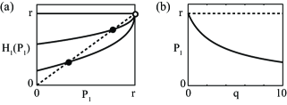
Figure 1: (a) (solid lines) The right hand side of the self-consistent equation when $q=0$, 1, and 10, from top to bottom. Dotted line is the left hand side of the equation. Filled and empty circles are stable and unstable solutions respectively. (b) Unstable (dashed line) and stable (thick line) solutions of the self-consistent equation.

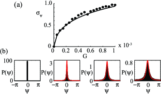
Figure 2: (a) Width of $P\left(\psi\right)$ as a function of the coupling strength $G$. The width is calculated from both theoretically (solid line) and numerically (filled circles). (b) $P\left(\psi\right)$ calculated numerically when $G=0.0$, 0.2, 0.5, and 1.0 $(\times 10^{-3})$, from left to right. Solid lines (online red) are theoretical predictions, Eq. (9).

We now examine the above result using the simplest example where $T=2\pi$ and $Z\left(\phi\right)=1-\cos\phi$. This phase response function is obtained directly from the quadratic integrate-and-fire neuron, which is also known as the theta-neuron or the Ermentrout-Kopell canonical modelermentrout_kopell . Putting $\left|Z_{1}\right|=1/2$ and $\left|Z_{n}\right|=0$ for $n>1$ to Eq. (10), we obtain the self-consistent equation for a variable $P_{1}$ as $P_{1}=\left(1-\sqrt{1-W_{1}^{2}}\right)/(2\pi W_{1})=H_{1}\left(P_{1}\right)$. To ensure $P\geq 0$, the condition $P_{1}\leq r$ is required. We plot each sides of the self-consistent equation in Figure 1 for various values of $q$. When $q=0$, there is no coupling in the network, the two lines have one intersection at $P_{1}=r$. Inserting the solution to Eq. (9) gives $P\left(\psi\right)=\delta\left(\psi\right)$, which exactly recover the previous result that single neurons always response precisely and that single oscillators always synchronize in-phase by common noiseteramae . Note that the Fourier series of $P$ is infinite while only the 1st component appears in the self-consistent equation. When $q>0$, i.e. there are finite couplings in the network, the solution $P_{1}=r$ turns out to be unstable and another stable solution appears in $P_{1}<r$. Inserting the solution to Eq. (9), we obtain the distribution with a finite width. As we increase $q$, i.e. increase coupling strength $G$, the width increases monotonically. We plot the evolution of the width in Figure 2a. In parallel to the analysis, we simulate Eq. (2) directly and plot the result also in Figure 2a. Numerical results are well fitted by the theoretical curve. Figure 2b shows distribution functions $P$ obtained from both numerical and theoretical calculations. Theoretical predictions agree fairly well with numerical results.

Positive width obtained here implies that networks of oscillators, in contrast to a single oscillator, do not synchronize perfectly across trials even though every trial is driven by the same input. Even if all the constituents, i.e. single oscillators here, are faithful to the input, it is not the case for the system as a whole. Spike sequence generated by the network is thus not perfectly the same across trials. Instead, the result implies enough coherence of spike trains between different trials, as indicated by the huge peak of the distribution around $\psi=0$. The width of the peak measures a degree of the coherence, up to which spike trains can be used reliably. Furthermore, the result tells us how the coherence changes qualitatively as a function of the coupling strength in the network.

If the network encodes information with precise spikes with temporal precision $\Delta\psi$ and that the information is decoded by a downstream neuron innervated by $K$ neurons in the network, reliability for the decoder neuron is roughly estimated as $\left(P\left(0\right)\Delta\psi\right)^{K}$, which rapidly goes to zero as $K$ increases, except if G is close to zero. Therefore the result infers that population codes based on precise spike times require weak or sparse mutual couplings in the network.

As the second example, we consider a coupled network of the Hodgkin-Huxley neuronshodgkin_huxley52 . We numerically integrate the system, Eq. (1), and compare the results predicted by theory. Since the Fourier component $Z_{n}$ of the neuron decays rapidly to zero when $n>5$, we use only the first 5 components to solve Eq. (10). To realize the Stratonovich situation in the numerical simulation, we use the Ornstein-Uhlenbech process with a correlation time $\tau=1$, which is sufficiently small comparing to the period of the oscillation. Figure 3 shows the result. As similar to the previous example, the distribution starts from the delta-function when $G=0$ and grows to a distribution with a finite width. The theory agrees well with numerical results, especially when the width of the distribution is small.

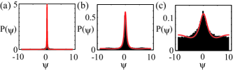
Figure 3: Distribution $P\left(\psi\right)$ of Hodgkin-Huxley neuron with mean current strength $I=6.5~{}mA/cm^{2}$. calculated numerically from Eq. (1) for $G=10^{-3}$ (a), $10^{-2}$ (b), and $10^{-1}$ (c). Solid lines (online red) are theoretical predictions.

We have assumed the balanced couplings, i.e., $\left<g_{ij}\right>=0$. If the couplings are not balanced, coefficient $A_{2}$ acquire additional terms, which in turn modify the self-consistent equation. Such biased couplings may significantly change the intra-network synchronization property of oscillators gerstner96 , which presumably influences the spike precision or the synchronization across trials. It is intriguing to extend the present analysis to the case with $\left<g_{ij}\right>\neq 0$.

Since the self-consistent equation has a unique stable solution, the obtained distribution is always realized over repeated trials even if initial phase differences between trials are infinitesimally small. This property reminds us of chaos theory in dynamical systems, in which a small difference between orbits increases rapidly until it roughly converges to a finite value characterized by the size of chaotic attractors. Recent studies suggested that neuronal circuits can be chaotic in a manner useful for computationsliquid ; vreeswijk ; battaglia07 . It remains fascinating whether our results reveal an active role of chaos in the brain.

We thank Y. Tsubo for fruitful discussions, H. Wang for careful reading of the manuscript, and Y. Kuramoto for helpful comments. The present work was supported by Kakenhi (B) 50384722 and 17022036.

References

- (1) H. L. Bryant and J. P. Segundo, J. Physiol. 260, 279 (1976); Z. F. Mainen and T. J. Sejnowski, Science 268, 1503 (1995).
- (2) P. Tiesinga, J. M. Fellous, and J. Sejnowski, Nat. Rev. Neurosci. 9, 97 (2008).
- (3) J. Teramae and D. Tanaka, Phys. Rev. Lett. 93, 204103 (2004); Prog. Theor. Phys. Suppl. 161, 360 (2006).
- (4) D. S. Goldobin and A. Pikovsky, Phys. Rev. E 71, 045201(R) (2005); Phys. Rev. E 73, 061906 (2006);
- (5) H. Nakao, K. Arai, and Y. Kawamura, Phys. Rev. Lett. 98, 184101 (2007).
- (6) A. Uchida, R. McAllister, and R. Roy, Phys. Rev. Lett. 93, 244102 (2004).
- (7) I. Z. Kiss, J. L. Hudson, J. Escalona, and P. Parmananda, Phys. Rev. E 70, 026210 (2004).
- (8) T. Zhou, L. Chen, and K. Aihara, Phys. Rev. Lett. 95, 178103 (2005).
- (9) R F. Galán, N. Fourcaud-Trocmé, G. B. Ermentrout, and N. N. Urban, J. Neurosci. 26, 3646 (2006).
- (10) A. Utagawa, T. Asai, T. Hirose and Y. Amemiya, IEICE T. Fund. Electr. E91, 2475 (2008).
- (11) R. L. Stratonovich, Topics in the Theory of Random Noise (Gordon and Breach, New York, 1963).
- (12) Y. Kuramoto, Chemical Oscillation, Waves, and Turbulence (Springer-Verlag, Tokyo, 1984); (Dover Edition, 2003).
- (13) Y. Kuramoto, unpublished.
- (14) G. B. Ermentrout, R. F. Galan, and N. N. Urban, Phys. Rev. Lett. 99, 248103, (2007).
- (15) D. J. Amit and N. Brunel, Cerebral. Cortex 7, 237, (1997); N. Brunel, J. Comput. Neurosci. 8, 183 (2000).
- (16) G. B. Ermentrout and N. Copell, SIAM J. Appl. Math. 46, 233, (1986); G. B. Ermentrout, Neural. Compt. 8, 979, (1996); N. Brunel, and P. E. Latham, Neural Comput. 15, 2281 (2003).
- (17) A. L. Hodgkin and H. Huxley, J. Physiol. 117, 500, (1952).
- (18) W. Gerstner, J. L. van Hemmen, J. D. Cowan, Neural Comput. 8, 1653 (1996).
- (19) W. Maass, T. Natschläger, and H. Markram, Neural Comput. 14, 2531 (2002); H. Jaeger and H. Haas Science 304, 78 (2004).
- (20) C. van Vreeswijk, and H. Sompolinsky, Science 274, 1724 (1996); Neural Comput. 10, 1321 (1998).
- (21) D. Battaglia, N. Brunel, and D. Hansel, Phys. Rev. Lett. 99, 238106 (2007).