Phase coupling estimation from multivariate phase statistics

Abstract

Coupled oscillators are prevalent throughout the physical world. Dynamical system formulations of weakly coupled oscillator systems have proven effective at capturing the properties of real-world systems. However, these formulations usually deal with the ‘forward problem’: simulating a system from known coupling parameters. Here we provide a solution to the ‘inverse problem’: determining the coupling parameters from measurements. Starting from the dynamic equations of a system of coupled phase oscillators, given by a nonlinear Langevin equation, we derive the corresponding equilibrium distribution. This formulation leads us to the maximum entropy distribution that captures pair-wise phase relationships. To solve the inverse problem for this distribution, we derive a closed form solution for estimating the phase coupling parameters from observed phase statistics. Through simulations, we show that the algorithm performs well in high dimensions (d$=$100) and in cases with limited data (as few as 100 samples per dimension). Because the distribution serves as the unique maximum entropy solution for pairwise phase statistics, the distribution and estimation technique can be broadly applied to phase coupling estimation in any system of phase oscillators.

Many complex natural phenomena can be modeled as networks of coupled oscillators. Examples can be drawn from the physical, chemical, and biological world. Oscillator models have been effective at describing the dynamics of coupled pendula, coupled Josephson junctions, reaction diffusion systems, circadian rhythms, oscillating neural networks, and even the coupling of firefly luminescence (see e.g. Buzsaki (2006); Kuramoto (1984); Mirollo and Strogatz (1990); Strogatz (2003); Winfree (2001)).

In many systems, coupling topology and the strength of interaction between network elements is of central scientific interest. However, network coupling often can not be measured directly and must be inferred from measurements. Therefore the inverse problem, or inferring network coupling from measurements, is of central importance.

In statistical mechanics, the inverse problem is typically solved by proposing a probability distribution and estimating the distribution’s parameters from measurements. A natural choice for the estimation, a highly under-determined problem, is given by the unique maximum entropy distribution that reproduces the statistics of the measurements Jaynes (1957). A number of such distributions and estimation techniques are used throughout the science and engineering communities. In the real-valued case the multivariate Gaussian distribution, and in the binary case the Ising model, serve as widely used multivariate maximum entropy distributions consistent with second order statistics. Each of these cases has well known estimation techniques for inferring the distribution’s parameters from observations. The availability of these techniques has led to a number of applications, e.g. the Ising model and its corresponding estimation techniques have been used to infer the coupling in networks of retinal ganglion cells Shlens et al. (2006); Schneidman et al. (2006). However, for the phase variables that are of interest in networks of oscillators there has been little work on providing a corresponding multivariate probabilistic distribution, or deriving estimation techniques to infer the distribution’s parameters from data.

In this Letter, we provide a solution to the inverse problem for systems of coupled phase oscillators. We begin by presenting the Langevin dynamics for a generalized form of the Kuramoto model of coupled phase oscillators. Solving for the equilibrium distribution yields a multivariate probability distribution of coupled phase variables. This probabilistic formalism allows us to derive a novel estimation technique for the coupling terms from phase variable measurements. We show that this technique performs robustly with limited data and in high dimensions.

Consider a network of $d$ identical coupled oscillators with intrinsic frequency $\omega$. In the limit of weak coupling, the amplitude of the oscillators can be assumed to be constant and the equations of motion can be formulated in terms of $d$ phase variables $0\!\leq\!\theta_{i}\!<\!2\pi$, $i\!=\!1,\ldots,d$. A popular choice for the dynamics of such a system is given by the Kuramoto model Kuramoto (1984), which has constant coupling between oscillators. We can generalize this model to include inhomogeneous couplings and inhomogeneous phase offsets between oscillators. The dynamic equation is then given by

$$\frac{\partial}{\partial t}\theta_{i}(t)\!=\omega-\kappa_{ij}\sum_{j=1}^{d}\!\sin(\theta_{i}(t)\!-\!\theta_{j}(t)\!-\!\mu_{ij})+\Gamma_{i}(t),$$ (1)

where $\kappa_{ij}$ is the coupling strength and $\mu_{ij}$ is the preferred phase between two oscillators $i$ and $j$. We only consider the case of symmetric coupling ($\kappa_{ij}\!=\!\kappa_{ji}$, $\mu_{ij}\!=\!-\mu_{ji}$). The noise fluctuations, $\Gamma_{i}(t)$, are zero mean Gaussian distributed with $\delta$ covariance functions and variance $\beta^{-1}$, corresponding to the temperature of the system:

$$\langle\Gamma_{i}(t)\rangle=0,\quad\langle\Gamma_{i}(t)\Gamma_{j}(t^{\prime})\rangle=2\,\beta^{-1}\delta_{ij}\delta(t-t^{\prime})\,.$$ (2)

The equations of motion (1) for our system of coupled oscillators can be considered as a nonlinear Langevin equation describing Brownian motion on a $d$-torus in the presence of the potential $E(\boldsymbol{\theta})$ given by

$$E(\boldsymbol{\theta})=-\frac{1}{2}\sum_{i,j=1}^{d}\kappa_{ij}\cos(\theta_{i}-\theta_{j}-\mu_{ij})\,,$$ (3)

where $\boldsymbol{\theta}$ is now a $d$-dimensional vector with components $\theta_{i}$. Note that by applying the transformation $\tilde{\theta}_{i}(t)\!=\!\theta_{i}(t)-\omega t$ to (1) we can assume $\omega\!=\!0$ without loss of generality.

By changing the coordinates from the angular representation, $\boldsymbol{\theta}$, to the complex representation, $\{\mathbf{x}\!\in\!\mathbb{C}^{d}\,\boldsymbol{|}\,|x_{k}|\!=\!1\}$ with components $x_{k}=e^{i\theta_{k}}$, we can rewrite eq. (3) more compactly as the (real-valued) quadratic Hermitian form:

$$E(\mathbf{x})=-{\textstyle\frac{1}{2}}\,\mathbf{x}^{\dagger}\mathbf{K}\mathbf{x}\,,$$ (4)

where $\mathbf{K}$ is a $d\!\times\!d$ Hermitian matrix with elements $K_{jk}=\kappa_{jk}e^{i\mu_{jk}}$. This energy function (3) is closely related to the XY-model, which only has homogeneous nearest neighbor couplings ($k_{ij}$ = const.) and no phase offsets ($\mu_{ij}$=0). This generalization is analogous to the extension of the homogeneous Ising model to spin glasses.

It is known (see e.g. Risken (1989)) that the probability density $p(\boldsymbol{\theta}(t),t)$ of a system governed by Langevin dynamics evolves according to the Fokker-Planck equation

$$\frac{\partial p(\boldsymbol{\theta},t)}{\partial t}=-\sum_{i}\frac{\partial}{\partial\theta_{i}}D_{i}p(\boldsymbol{\theta},t)+\sum_{ij}\frac{\partial^{2}}{\partial\theta_{i}\partial\theta_{j}}D_{ij}p(\boldsymbol{\theta},t)\,,$$ (5)

with drift and diffusion coefficients given by

$$D_{i}=-\frac{\partial E(\boldsymbol{\theta})}{\partial\theta_{i}},\quad D_{ij}=\beta^{-1}\delta_{ij}\,.$$ (6)

Since the drift coefficient $D_{i}$ is a gradient field and the diffusion coefficient $D_{ij}$ is constant, we can solve the Fokker-Planck equation (5) for the stationary solution in closed form and obtain

$$p(\boldsymbol{\theta})=\frac{1}{Z(\mathbf{K})}\exp[-\beta E(\boldsymbol{\theta})]$$ (7)

with the the energy function $E(\boldsymbol{\theta})$ given by (3), and partition function $Z(\mathbf{K})$.

We wish to solve the inverse problem for the general case of coupled phase oscillators in equation (7). Stated explicitly, the problem is to infer the distribution’s parameters (coupling terms $\kappa_{ij}$ and phase offsets $\mu_{ij}$) from measurements of the network’s state, $\boldsymbol{\theta}$.

The inverse problem is typically solved by following a maximum likelihood estimation procedure. Given the likelihood function $q(\boldsymbol{\theta})$ and the data distribution $p(\boldsymbol{\theta})$, the maximum likelihood of the observed data with respect to the distribution parameters can be computed by setting the derivative of the log-likelihood function to zero,

$$\frac{\partial\langle\log q(\boldsymbol{\theta})\rangle_{p(\boldsymbol{\theta})}}{\partial K_{ij}}\!\!=-\bigg{\langle}\frac{\partial E}{\partial K_{ij}}\bigg{\rangle}_{p(\boldsymbol{\theta})}\!\!+\bigg{\langle}\frac{\partial E}{\partial K_{ij}}\bigg{\rangle}_{q(\boldsymbol{\theta})}\!\!\stackrel{{\scriptstyle!}}{{=}}\,0\,,$$ (8)

where $\langle\ldots\rangle_{q(\boldsymbol{\theta})}$ denotes the expectation value taken over the distribution $q(\boldsymbol{\theta})$. In our situation, a closed form solution to this equation does not exist. However, we can find a solution by iteratively descending the gradient. This procedure has a number of drawbacks: the procedure is inherently iterative, estimating the expectation under the estimated distribution $q(\boldsymbol{\theta})$ in equation (8) involves a computationally expensive sampling procedure, and the sampling procedure may suffer from a variety of problems due to the landscape of the energy function.

To avoid the pitfalls of the maximum likelihood approach, we now derive a closed form solution to the inverse problem for phase coupled oscillators. We use the score-matching method introduced by Hyvarinen Hyvärinen (2005, 2007). Score-matching allows the fitting of probability distributions of the exponential form for real-valued data without computation of the normalization constant $Z$. If the energy depends linearly on the distribution parameters, the solution can be computed in closed form by setting the derivative of the score function to zero Hyvärinen (2007).

We follow this approach to estimate the distribution parameters for our distribution in equation (7). The score matching estimator of $\mathbf{K}$ is given by $\widehat{\mathbf{K}}=\arg\min_{\mathbf{K}}J_{\mathrm{SM}}(\mathbf{K})$ and the score function $J_{\mathrm{SM}}(\mathbf{K})$ is given by

$$J_{\mathrm{SM}}(\mathbf{K})=\left\langle\textstyle{\frac{1}{2}}[\nabla_{\boldsymbol{\theta}}E(\boldsymbol{\theta})][\nabla_{\boldsymbol{\theta}}E(\boldsymbol{\theta})]^{T}-\nabla_{\boldsymbol{\theta}}^{2}E(\boldsymbol{\theta})\right\rangle$$

with the expectation value, $\langle\ldots\rangle$, taken over the data distribution. Using the quadratic form of the energy in (7) and the Jacobian $D_{ij}:=\partial x_{i}/\partial\theta_{j}$, we compute

$$\nabla_{\boldsymbol{\theta}}E = -\textstyle{\frac{1}{2}}\mathbf{x}^{\dagger}\mathbf{K}\mathbf{D}-\textstyle{\frac{1}{2}}\mathbf{D}^{\dagger}\mathbf{K}\mathbf{x}$$

$$\nabla_{\boldsymbol{\theta}}^{2}E = \mathbf{x}^{\dagger}\mathbf{K}\mathbf{x}-\mathrm{Tr}(\mathbf{D}^{\dagger}\mathbf{K}\mathbf{D})=-2\,E$$

$${}[\nabla_{\boldsymbol{\theta}}E]{}[\nabla_{\boldsymbol{\theta}}E]^{T} = \textstyle{\frac{1}{2}}\mathbf{x}^{\dagger}\mathbf{KK}\mathbf{x}+\textstyle{\frac{1}{4}}\mathbf{x}^{\dagger}\mathbf{KD}\mathbf{D}^{T}\mathbf{K}^{T}\mathbf{x}^{*}$$

$$+\textstyle{\frac{1}{4}}\mathbf{x}^{T}\mathbf{K}^{*}\mathbf{D}^{*}\mathbf{D}^{\dagger}\mathbf{K}\mathbf{x}$$

The estimator $\widehat{\mathbf{K}}$ is computed by setting the derivative of the score function $\partial/\partial K_{ij}\,J_{\mathrm{SM}}(\mathbf{K})$ to zero. This produces a system of linear equations,

$$\sum_{k,l=1}^{d}(\delta_{jl}C_{ik}+\delta_{ik}C_{lj}-\delta_{jk}C_{iljk}-\delta_{il}C_{iljk})\,\widehat{K}_{kl}=4\,C_{ij},$$ (9)

where the expectation values are defined as $C_{ij}\!=\!\langle x_{i}x_{k}^{*}\rangle$ and $C_{ijkl}\!=\!\langle x_{i}x_{j}x_{k}^{*}x_{l}^{*}\rangle$. We can solve this system of linear equations using standard techniques.

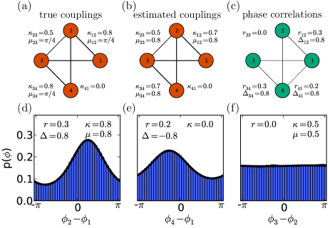
Figure 1: Phase coupling estimation recovers the true coupling from measurements. (a) Diagram of four coupled phase oscillators. (b) Estimated coupling parameters using phase coupling estimation. (c) Pair-wise phase correlations of the oscillators in a. Phase correlations are parameterized by the mean direction vector $r_{kl}e^{i\Delta_{kl}}\!=\!\langle e^{i\theta_{l}}e^{-i\theta_{k}}\rangle$ with amplitude $r_{kl}$ and angle $\Delta_{kl}$. (d) Empirical phase distribution of the phase difference between oscillators 1 and 2. The empirical distribution is highly concentrated in the difference of the phases, while the marginals are flat (not shown). Phase correlations and estimated couplings are given. (e) Distribution of phase differences of oscillators 1 and 4, which are not directly coupled. (f) Uniform distribution of phase differences of oscillators 2 and 3, which are directly coupled.

In the following, we show that phase coupling estimation recovers the parameters of simulated Kuramoto models. We begin by simulating a system of four oscillators using equation (1) with couplings shown in Fig. 1a. Given samples of the simulated phase variables $\boldsymbol{\theta}$, we compute the correlations, $C_{ij}$, and required four-point functions, $C_{ijkl}$, and invert the linear system in equation (9). This produces an estimate of the coupling parameters. Phase coupling estimation recovers the true coupling parameters as shown in Fig. 1b.

We would like to point out that the pairwise statistics in systems of coupled phase oscillators are only indirectly related to the coupling parameters. Phase correlations, a pair-wise measurement often used to characterize oscillator systems, have a direct relationship to the marginal distribution of phase differences but not to coupling parameters. The form of the marginal distribution can be derived by examination of the individual factors in the definition

$$p(\theta_{k}\!-\!\theta_{l})\sim\int\prod_{i,j=1}^{d}\exp\left[\kappa_{ij}\cos(\theta_{i}-\theta_{j}-\mu_{ij})\right]\mathrm{d}\theta^{d-2}\,,$$ (10)

in which the integration is over all phases $\theta_{i}$ with $i\!\neq\!k,l$. After applying the variable substitution $\tilde{\theta}_{i}\!=\!\theta_{i}+\theta_{l}$, all terms in (10) either depend on the phase difference $\theta_{k}\!-\!\theta_{l}$, or are independent of $\theta_{k}$ and $\theta_{l}$. The independent terms integrate to a constant and the remaining terms combine to a von Mises distribution in the pairwise phase difference

$$p(\theta_{k}\!-\!\theta_{l})=\frac{1}{Z(\gamma_{kl})}e^{\displaystyle\gamma_{kl}\cos(\theta_{k}\!-\!\theta_{l}\!-\!\Delta_{kl})},$$ (11)

with mean phase $\Delta_{kl}$ and concentration parameter $\gamma_{kl}$. The concentration parameter $\gamma_{kl}$ can be obtained by numerically solving the equation $r_{kl}\!=\!I_{1}(\gamma_{kl})/I_{0}(\gamma_{kl})$ and the normalization constant $Z(\gamma_{kl})$ is given by $Z(\gamma_{kl})\!=\!2\,\pi I_{0}(\gamma_{kl})$. $I_{0}(x)$ and $I_{1}(x)$ denote the modified Bessel functions of zeroth and first order, respectively. The value of $\gamma_{kl}$ is related to the coupling parameters $\mathbf{K}$ through equation (10). Therefore, there is a non-trivial relationship between the measured phase correlations and the coupling parameters.

Because of this non-trivial relationship, pair-wise measurements can often lead to false interpretations of the true coupling. We show the measured phase correlations of our four oscillator system in Fig. 1c. Phases $\theta_{1}$ and $\theta_{4}$ show clear correlations even though they are not directly coupled to each other (see Fig. 1e). Conversely, phases $\theta_{2}$ and $\theta_{3}$ are strongly coupled but are uncorrelated (see Fig. 1f).

We now systematically analyze the performance of phase coupling estimation: the ability of the technique to recover the distribution parameters from data. The procedure is as follows. We begin by sampling a set of distribution parameters $\mathbf{K}$. Given these parameters we then sample phase variables by numerically integrating (1). We then estimate the parameters given the sampled data using equation (9). The real and imaginary entries of the complex matrix $\mathbf{K}$ are sampled from a normal distribution: $\mathrm{Re}\{K_{ij}\},\mathrm{Im}\{K_{ij}\}\sim N(0,1)$ and the diagonal entries are set to zero: $K_{ii}=0$. Note that this produces a dense coupling matrix.

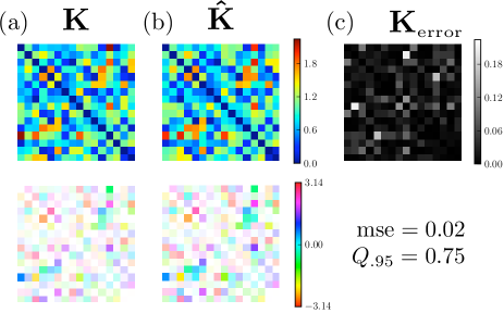
Figure 2: Phase coupling estimation for a system of 16 coupled oscillators with random coupling. (a) True coupling matrix $\mathbf{K}$: true system parameters for $d=16$ (first row, element-wise amplitude; second row, element-wise angle with alpha channel scaled by the amplitude of the corresponding element, best viewed in color). (b) estimated coupling matrix $\mathbf{\hat{K}}$: estimated parameters recovered from $2560$ time samples of $\boldsymbol{\theta}$ using equation (9). (c) estimation error: first row element-wise mse (note scaling), second row estimation error measurements, mse and $Q_{.95}$ (see text for definition).

In the first column of Fig. 2, we graphically display the element-wise amplitude and phase of a sample matrix $\mathbf{K}$ where $d\!=\!16$. Using this matrix we sampled $N\!=\!2560$ phase vectors. The recovered parameters are shown in the second column of Fig. 2. While it is clear that these matrices are visually similar, we quantified the error using two different metrics. First we calculate the mean-squared-error of the matrix elements, $\text{mse}\!=\!\frac{1}{2d^{2}}\sum_{i,j}{|K_{ij}\!-\!\hat{K}_{ij}|^{2}}$, where $\hat{K}_{ij}$ is the estimated parameter. In the third column of Fig. 2 we display the element-wise error before averaging. We also computed a metric indicating the quality of the recovered parameters borrowed from Ref. Timme (2007): $Q_{.95}\!=\!\frac{1}{d^{2}}\sum_{i,j}u(1\!-.95\Delta K_{ij})$, where $\Delta K_{ij}=|K_{ij}-\hat{K}_{ij}|/2K_{\max}$, $u$ is the Heaviside step function, and $K_{\max}$ is the maximum absolute value of all matrix entries $K_{ij}$ and $\hat{K}_{ij}$. For the example in Fig. 2, $\text{mse}\!=\!0.02$, and $Q_{.95}=0.75$.

We computed these error metrics over a range of dimensions and samples per dimension. The error metrics for each dimension and samples per dimension were averaged over 20 trials and are plotted in Fig. 3. The algorithm achieves highly accurate parameter recovery for as few as 100 samples per dimension and achieves full recovery of parameters as the number of samples per dimension reaches 1000. This indicates that recovery of true parameters is quite feasible in many real world settings.

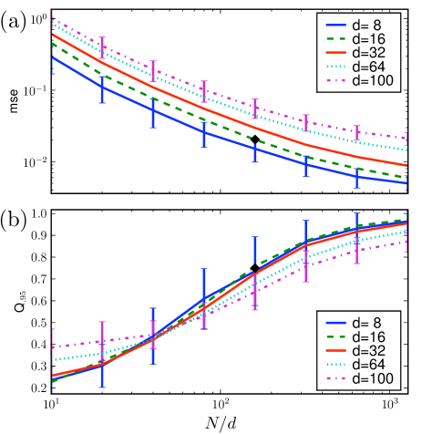
Figure 3: Performance of phase coupling estimation. (a) mean-squared-error,  mse, metric as a function of samples per dimension for various dimensions, $d=8,16,32,64,100$. (b) $Q_{.95}$ metric. The example displayed in Fig. 2 is indicated by the black diamond. Values are averaged over 20 trials. For visual clarity, standard error bars are only displayed for $d=8$ and $d=100$. Phase coupling estimation accurately recovers the system parameters with only 100 samples per dimension and achieves nearly perfect recovery with 1000 samples per dimension.

In this Letter we have introduced a closed form solution to the inverse problem for systems of coupled phase oscillators using a maximum entropy approach. We close by pointing out the relation of our work to other attempts at solving the inverse problem for coupled phase oscillators. Previous examples of probabilistic distributions of phase variables only characterize univariate or bivariate distributions (see e.g. Jammalamadaka and Sengupta (2001); Mardia and Jupp (2000)). Distributions similar to equation (7) have not been extended to dimensions beyond $d\!=\!2$ Gatto and Jammalamadaka (2007); Mardia et al. (2007). Common multivariate phase distributions do not capture the statistics that are relevant for coupled phase oscillators. Most notably the von Mises-Fisher distribution only captures a unimodal phase distribution on the hyper-sphere, which does not produce unimodal concentrations in the differences of phase variables. One of the most relevant proposals is the estimation procedure of Timme Timme (2007). While the method of Ref. Timme (2007) successfully recovers the coupling parameters, it requires repeated intervention, which may not be feasible in many real-world experiments.

Phase coupling estimation can potentially provide a contribution in a variety of situations of scientific interest. Because our phase coupled estimation technique derives the unique maximum entropy solution, it serves as the least biased estimate of the system possible and can be used when the true dynamics of the system are unknown. Such situations are prevalent in neuroscience where oscillations are thought to mitigate cognitive processes but the form of the underlying dynamical system is unknown. This field has lacked a suitable procedure for estimating phase interactions and has largely relied on pair-wise statistical measurements (see e.g. Varela et al. (2001)).