Properties of the Scalar Mesons below 1.0 GeV as Hadronic Molecules

Abstract

Properties of scalar mesons below 1.0 GeV have been studied by regarding them as hadronic molecular states. Using the effective Lagrangian approach, we have calculated their leptonic decays, strong decays and productions via the $\phi$ meson radiative decays. Comparing our results with that given in the literature and the data, we conclude that it is difficult to arrange them in the same nonet if some of them are pure hadronic molecules.

I Introduction

Understanding the nature of scalar mesons is a prominent topic in the past 30-40 years. The importance of the nature of the scalar mesons is that, because the properties of the scalar mesons, especially that with masses below 1.0 GeV, are difficult to be understood in the constituent quark models, the study of the light scalar mesons can help us to understand the nonperturbative properties of QCD. Moreover, because the scalar mesons have the same quantum numbers as the vacuum, it can help us to reveal the mechanism of symmetry breaking which is, up to now, one of the most profound problems in particle physics.

Many properties of scalar mesons are not so clear although they have been investigated for several decades. Experimentally, it is difficult to identify the scalar mesons because of their large decay widths which cause strong overlaps between resonances and grounds and also because several decay channels open up within a short mass interval. And due to these problems many data on scalar mesons are not so precise, so that it is not so easy to reveal their underlying structures Amsler:2008zz ; Godfrey:1998pd ; Close:2002zu . Theoretically, there are many calculations based on different models, but it seems that one cannot rule out some of them based on the present measurements. Currently, the observation shows that the known $0^{++}$ mesons below 2.0 GeV can be classified into to classes: One class with masses below (or near) 1.0 GeV and the other class with masses above 1.0 GeV Amsler:2008zz .

To study light scalar mesons, one problem we have to confront is how to classify the present observed scalar objects. One opinion is that the scalar objects with masses below 1.0 GeV, including two isosinglets $\sigma(600)$ and $f_{0}(980)$, one isotriplet $a_{0}(980)$ and two isodoublets $K_{0}^{\ast}(800)$, can be classified into one nonet Jaffe:1976ig ; Jaffe:1976ih ; Oller:1998hw ; Ishida:1999qk ; Alford:2000mm ; Maiani:2004uc ; Scadron:2003yg . On the contrary, another opinion, inspired by linear sigma model and unitary quark model, is that $\sigma(600),f_{0}(980),a_{0}(980)$ and $K_{0}^{\ast}(1430)$ form a scalar nonet Tornqvist:1995kr ; Tornqvist:1999tn .

Concerning the structures of light scalar mesons, they are still open questions so far although many attempts have been made to understand them in the literature. For the light scalars mesons with masses below 1.0 GeV, some people, by considering their dominant two-body decays, believe that they are multiquark (or multiquark dominant) states  Jaffe:1976ig ; Jaffe:1976ih ; Weinstein:1990gu ; Alford:2000mm ; Maiani:2004uc ; Pelaez:2004xp ; Pelaez:2003dy ; Pelaez:2006nj or hadronic molecular states Weinstein:1990gu ; Giacosa:2007bs ; Branz:2007xp ; Branz:2008qm ; Branz:2008ha ; Branz:2008cb ( Note that some references list here do not different multiquak state from molecular state.). Alternatively, properties of some of these light scalar mesons were also investigated in the $q\bar{q}$ picture Tornqvist:1995kr ; Faessler:2003yf ; vanBeveren:2001kf ; Celenza:2000uk . Moreover, in Ref. Dai:2003ip , the spectrum of light scalar mesons below 1.0 GeV were studied in the $q\bar{q}$ picture with including the instanton effect. And it was found that the $q\bar{q}$ components with the instanton or tetraquark effect can explain the spectrum at a certain level. In Ref. :2008my , we also studied the the effect of instanton-induced interaction in light meson spectrum on the basis of the phenomenological harmonic models for quarks. For the light scalar mesons with masses above 1.0 GeV, the potential model calculation indicates that they are $q\bar{q}$ states. However, concerning the spectrum of the scalar mesons with masses above 1.0 GeV, since there are three isoscalar states, $f_{1}(1370),f_{0}(1500)$ and $f_{0}(1710)$, one believes that there is a glueball candidate among them. Based on the recent lattice results, the mixing between glueball and $q\bar{q}$ components in these three objects were fit in Ref. Cheng:2009dg . It should be noted that, the two problems we mentioned above are not independent. If we know the classification of the scalar mesons and the structures of some states, we may deduce the structures of other states according to the classification, and inversely, if the structures of the scalar mesons are confirmed the classification becomes obvious.

In this paper, since some scalar mesons (mainly $f_{0}(980)$ and $a_{0}(980)$) have been studied in the literature and the numerical results yielded there are consistent with the data, we will study the properties of all the scalar mesons with masses below 1.0 GeV by regarding all of them as pure hadronic molecules and check whether they form one nonet in the effective Lagrangian approach. Our logic is, if the scalar meson with masses below 1.0 GeV form a nonet, they should have the same structures. And if some of them can be interpreted as hadronic molecules as discussed in the literature Giacosa:2007bs ; Branz:2007xp ; Branz:2008qm ; Branz:2008ha ; Branz:2008cb , all the elements in the same nonet should be interpreted as hadronic molecules. If our start point is reasonable, the yielded results should be consistent with the data. Otherwise, it is difficult to classify them into the same nonet, at least in the the hadronic molecular interpretation.

In the molecular picture the interaction of scalar meson to its constituents can be described by the effective Lagrangian. The corresponding effective coupling constant $g_{{}_{S}}$ is determined by the compositeness condition $Z=0$ which was earlier used by nuclear physicists and is being widely used by particle physicists(see the references in Faessler:2007gv ). In Refs. Faessler:2007gv ; Faessler:2007us ; Dong:2008gb this method has been applied to study the newly observed charmed mesons Faessler:2007gv ; Faessler:2007us ; Dong:2008gb and the decay properties calculated there are consistent with the observed data. We had employed the above technique to predict the decay properties of the bottom-strange mesonsFaessler:2008vc and recently we applied this method to studied the baryonium picture of $X(1835)$ Ma:2008hc . The production and decay properties of some scalar mesons have been studied in Refs. Giacosa:2007bs ; Branz:2007xp ; Branz:2008qm ; Branz:2008ha ; Branz:2008cb with the help of this technique by regarding them as pure hadronic molecules and the numerical results yielded there agree with the data.

It should be mentioned that, in the tetraquark interpretation of the scalar mesons with masses below 1.0 GeV, the diquark $(qq)$ is in the $\underline{3}$ representation $(us,ds,ud)$ of $SU(3)$ group so there are at most two valence strange quarks in the $\sigma(600)$ and $f_{0}(980)$ as shown in Fig. 1. However in the hadronic molecular interpretation, an isosinglet $\eta$ constituent in addition to the isodoublet $(K^{+},K^{0})$ should be introduced to form a nonet. So that there is $\eta\eta$ component, or $(s\bar{s})(s\bar{s})$ at the quark level, in $\sigma(600)$ and $f_{0}(980)$ which makes it is difficult to understand the scalar meson spectrum from the quark level. Fortunately, in our present work we adopt the scalar meson spectrum as input, with the help of compositeness condition, to determine the coupling constant $g_{{}_{S}}$ between the molecule and its constituents.

In our explicit calculation of the effective coupling constant $g_{{}_{S}}$, we will consider two cases, the one is local interaction case and the other one is nonlocal interaction case with including a correlation function which describes the distribution of the constituents among the molecules. As in our previous works, we will introduce a typical scale parameter $\Lambda_{S}$ to describe the finite size of the molecules. The numerical results show, in the region where the coupling constant $g_{{}_{S}}$ is stable against $\Lambda_{S}$, the yielded value of $g_{{}_{S}}$ for the corresponding molecular scalar meson, is consistent with that yielded from the local interaction picture. So that in the other calculations we will take the local interaction vertex. For other interactions, we will resort to the phenomenological Lagrangian and borrow the relevant coupling constants from the existing literature.

To determine the mixing angle $\theta_{S}$ between $\sigma(600)$ and $f_{0}(980)$, we will apply the data for $f_{0}(980)\to 2\gamma$. It is natural that only with this data one cannot fix $\theta_{S}$ uniquely and to fix $\theta_{S}$ a well measured process of $\sigma(600)$, for example $\sigma(600)\to 2\gamma$, is necessary. Concerning that the coupling constant $g_{\sigma}$ depends on the mass of $\sigma(600)$ closely, we will not use this data, and will not discuss the physics of $\sigma(600)$ in the present work.

With the determined coupling constant $g_{{}_{S}}$ we will calculate leptonic decay constants of the scalar mesons and the relevant leptonic decay widths. And from the yielded numerical results, we find that the leptonic decay widths of the scalar mesons are too small to be measured at present. With our hadronic interpretation, the strong decays of the scalar mesons to two-pseudoscalar mesons have also been calculated. The numerical results for the strong decays indicate that it is difficult to arrange the scalar mesons with masses below 1.0 GeV into the same nonet in the hadronic molecular interpretation. To study the productions of the scalar mesons $f_{0}(980)$ and $a_{0}(980)$ in the radiative decays of $\phi$ meson, we will includ the final state interaction effect due to the two axial-vector mesons nonets with quantum numbers $J^{PC}=1^{++}$ and $1^{+-}$. We find the final state interaction plays a negligible role in the production rates.

This paper is organized as the following: In section II, we discuss the molecular structures of the light scalar nonet with masses below 1.0 GeV and calculate the coupling constant $g_{{}_{S}}$, the leptonic decay constants and the leptonic decay widths. In section III, the strong decays of the scalar mesons are calculated in the framework of effective Lagrangian approach. The productions of the $f_{0}$ and $a_{0}$ mesons in the radiative decays of $\phi$ meson are studied in section IV. Our discussions and conclusions are given in the last section.

II Molecular Structures of the Scalar Meson Nonet below 1.0 GeV

In this section, we will discuss the properties of the scalar meson nonet below 1.0 GeV in the hadronic molecular explanation, i.e., regarding them as two-pseudoscalar-meson bound states. At first, we will identify pseudoscalar meson contents of the scalar mesons and construct the effective Lagrangian describing the interaction between scalar meson and its constituents. Then the magnitude of the coupling constant $g_{{}_{S}}$ is calculated with the help of compositeness condition and the leptonic decay constants and the leptonic decay widths of the scalar mesons are yielded by the standard loop integral.

II.1 Molecular Structures of the Scalar Nonet

Now, we are in the position to identify the constituents of light scalar meson nonet as hadronic molecules. As we pointed above that we will accept the opinion that the light scalar mesons: two isosinglets $\sigma(600)$ and $f_{0}(980)$, one isotriplet $a_{0}(980)$ and two isodoublets $K_{0}^{\ast}(800)$, can be classified into one nonet, we should have three elements at least to form this nonet. And considering the physical requirement that the bound state should have a mass smaller than the threshold of the corresponding constituents, the constituents of the light scalar mesons should be $K^{+},K^{0}$ and $\eta$. With these considerations, we may arrange the two-pseudoscalar-meson bound states in the $(I_{3},Y)$ plane (where $Y$ is the hypercharge which is relative to the strangeness $S$ via relation $Y=S$ for mesons and relates the charge $Q$ and the third component of isospin $I_{3}$ via relation $Q=I_{3}+(1/2)Y$) as Fig. 1. As a comparison, we also illustrate the quark contents of the scalar nonet in the tetraquark interpretation in Fig. 1.

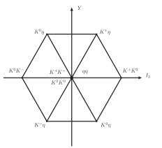
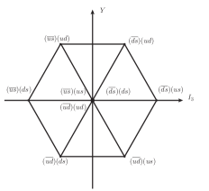
Figure 1: Hadronic molecules (left) and tetraquark explanations (right) of scalar mesons in the $(I_{3},Y)$ plane.

Comparing with the quantum numbers of the light scalar mesons, we write down the hadronic molecular structures of two isodoublets and isotriplet as

$$\left(\begin{array}[]{c}|K_{0}^{\ast+}(800)\rangle\\ |K_{0}^{\ast 0}(800)\rangle\\ \end{array}\right) = \eta\left(\begin{array}[]{c}K^{+}\\ K^{0}\\ \end{array}\right);\;\;\;\;\;\left(\begin{array}[]{c}|\bar{K}_{0}^{\ast 0}(800)\rangle\\ |K_{0}^{\ast-}(800)\rangle\\ \end{array}\right)=\eta\left(\begin{array}[]{c}\bar{K}^{0}\\ K^{-}\\ \end{array}\right)$$ (9)

$$\left(\begin{array}[]{c}|a_{0}^{+}(980)\rangle\\ |a_{0}^{-}(980)\rangle\\ \end{array}\right) = \left(\begin{array}[]{c}K^{+}\bar{K}^{0}\\ K^{0}K^{-}\\ \end{array}\right);\;\;\;\;\;|a_{0}^{0}(980)\rangle=\frac{1}{\sqrt{2}}(|K^{+}K^{-}\rangle-|\bar{K}^{0}K^{0}\rangle)$$ (14)

and two singlets as

$$S_{8} = \frac{1}{\sqrt{6}}(|K^{+}K^{-}\rangle+|K^{0}\bar{K}^{0}\rangle-2|\eta\eta\rangle)$$

$$S_{0} = \frac{1}{\sqrt{3}}(|K^{+}K^{-}\rangle+|K^{0}\bar{K}^{0}\rangle+|\eta\eta\rangle)$$ (15)

The physical states $\sigma(600)$ and $f_{0}(980)$ should be mixing states of $S_{8}$ and $S_{0}$ via the mixing angle defined as

$$\left(\begin{array}[]{c}f_{0}(980)\\ \sigma(600)\\ \end{array}\right) = \left(\begin{array}[]{cc}\cos\theta_{S}&\sin\theta_{S}\\ -\sin\theta_{S}&\cos\theta_{S}\\ \end{array}\right)\left(\begin{array}[]{c}S_{8}\\ S_{0}\\ \end{array}\right)$$ (22)

In terms of the constituents and the mixing angle $\theta_{S}$, the physical $\sigma(600)$ and $f_{0}(980)$ mesons can be expressed as

$$f_{0}(980) = (\frac{\cos\theta_{S}}{\sqrt{6}}+\frac{\sin\theta_{S}}{\sqrt{3}})(|K^{+}K^{-}\rangle+|K^{0}\bar{K}^{0}\rangle)+(\frac{\sin\theta_{S}}{\sqrt{3}}-\frac{2\cos\theta_{S}}{\sqrt{6}})|\eta\eta\rangle$$

$$\sigma(600) = (-\frac{\sin\theta_{S}}{\sqrt{6}}+\frac{\cos\theta_{S}}{\sqrt{3}})(|K^{+}K^{-}\rangle+|K^{0}\bar{K}^{0}\rangle)+(\frac{\cos\theta_{S}}{\sqrt{3}}+\frac{2\sin\theta_{S}}{\sqrt{6}})|\eta\eta\rangle$$ (23)

In the case of ideal mixing with $\cos\theta_{S}=\frac{1}{\sqrt{3}}$ and $\sin\theta_{S}=\sqrt{\frac{2}{3}}$ one has

$$f_{0}(980) = \frac{1}{\sqrt{2}}(|K^{+}K^{-}\rangle+|K^{0}\bar{K}^{0}\rangle);\;\;\;\;\;\;\sigma(600)=|\eta\eta\rangle$$ (24)

This is the case in which the hadronic molecular picture of $f(980)$ was studied in some literature, for example Refs. Branz:2007xp ; Branz:2008qm ; Branz:2008ha ; Branz:2008cb . In our present work, we will take the mixing angle as a parameter and fit it from the data in the following.

In summary, with the above discussions, one can write the scalar meson nonet in a matrix form as

$$S = \frac{1}{\sqrt{2}}\left(\begin{array}[]{ccc}a_{0}^{0}(980)+\frac{1}{\sqrt{6}}S_{8}+\frac{1}{\sqrt{3}}S_{0}&\sqrt{2}a_{0}^{+}(980)&\sqrt{2}K_{0}^{\ast+}(800)\\ \sqrt{2}a_{0}^{-}(980)&-a_{0}^{0}(980)+\frac{1}{\sqrt{6}}S_{8}+\frac{1}{\sqrt{3}}S_{0}&\sqrt{2}K_{0}^{\ast 0}(800)\\ \sqrt{2}K_{0}^{\ast-}(800)&\sqrt{2}\bar{K}_{0}^{\ast 0}(800)&-\sqrt{\frac{2}{3}}S_{8}+\frac{1}{\sqrt{3}}S_{0}\\ \end{array}\right)$$ (28)

And the ideal mixing reduces to

$$S_{\rm ideal} = \frac{1}{\sqrt{2}}\left(\begin{array}[]{ccc}a_{0}^{0}(980)+f_{0}(980)&\sqrt{2}a_{0}^{+}(980)&\sqrt{2}K_{0}^{\ast+}(800)\\ \sqrt{2}a_{0}^{-}(980)&-a_{0}^{0}(980)+f_{0}(980)&\sqrt{2}K_{0}^{\ast 0}(800)\\ \sqrt{2}K_{0}^{\ast-}(800)&\sqrt{2}\bar{K}_{0}^{\ast 0}(800)&\sqrt{2}\sigma(600)\\ \end{array}\right)$$ (32)

It should be noted that in the hadronic molecular interpretation there are more quark contents in the relevant scalars compared to the tetraquark interpretation as shown in Fig. 1. This makes it seems that it is difficult to understand the scalar meson spectrum in the molecular picture. However, at present, we do not attempt to calculate the scalar meson spectrum but take the scalar meson masses as input to determine the coupling constants.

The effective Lagrangian, without including the distribution of the constituents among the molecules, describing the interaction between the scalar mesons and their constituents can be written as

$${\cal L}_{S}^{\rm LC} = g_{{}_{S}}^{\rm LC}P^{{\dagger}}(x)S(x)P(x)$$ (33)

where the upper index ”LC” denotes the local interaction vertex, $S$ denotes the scalar meson matrix which was give in Eq. (28) and $P$ denotes the constituent pseudoscalar meson matrix

$$P = \left(\begin{array}[]{c}K^{+}\\ K^{0}\\ \eta\\ \end{array}\right)$$ (37)

To include the distribution function which illustrates the distribution of the constituents in the molecules, one should modify the interaction Lagrangian (33) as

$${\cal L}_{S}^{\rm NL} = g_{{}_{S}}^{\rm NL}\int d^{4}y\Phi_{S}(y^{2})P_{i}^{{\dagger}}(x+\omega_{j}y)S_{ij}(x)P_{j}(x-\omega_{i}y)$$ (38)

where the upper index NL denotes the nonlocal interaction vertex. It should be noted that to keep the $U(1)_{\rm em}$ gauge invariance, a Wilson’s line connecting the charged particles at different positions should be introduced. The kinematic parameter $\omega_{i}$ is defined as

$$\omega_{i} = \frac{M_{i}}{M_{1}+M_{2}}$$ (39)

with $M_{i}$ as the mass of $i-$th constituent. And correlation function $\Phi(y^{2})$ describes the distribution of the constituents in the molecule. The Fourier transform of the correlation function reads

$$\Phi(y^{2}) = \int\frac{d^{4}p}{(2\pi)^{4}}\tilde{\Phi}(p^{2})e^{-ip\cdot y}$$ (40)

In the following numerical calculations, an explicit form of $\tilde{\Phi}(p^{2})$ is necessary. Throughout this paper, we will take the Gaussian form

$$\tilde{\Phi}(p^{2}) = \exp(p^{2}/\Lambda_{S}^{2})$$ (41)

where the parameter $\Lambda_{S}$ is a size parameter which parametrizes the distribution of the constituents inside the molecule. The magnitude of $\Lambda_{S}$ is determined by requiring that the effective coupling constant $g_{{}_{S}}^{\rm NL}$ should be stable against it. It should be noted that the choice (41) is not unique. In principle any choice of $\tilde{\Phi}(p^{2})$, as long as it renders the integral convergent sufficiently fast in the ultraviolet region, is reasonable. In this sense, $\tilde{\Phi}(p^{2})$ can be regarded as a regulator which makes the ultraviolet divergent integral well defined. In addition, we would like to point out that, in the limit $\Phi(y^{2})\to\delta^{4}(y)$, the interaction between the scalar meson and its constituents becomes a local one, i.e., Eq. (38) approaches to Eq. (33).

II.2 The Effective Coupling Constant Between the Scalar Meson and its Constituents

After the discussion on the interaction Lagrangian of the scalar meson and its constituents, we are ready to calculate the effective coupling constant $g_{{}_{S}}$ with the help of the compositeness condition

$$Z_{S} = 1-g_{{}_{S}}^{2}\Sigma_{S}^{\prime}(m_{S}^{2};M_{1}^{2},M_{2}^{2})=1-g_{{}_{S}}^{2}\frac{d}{dq^{2}}\Sigma_{S}(q^{2};M_{1}^{2},M_{2}^{2})\bigg{|}_{q^{2}=m_{S}^{2}}=0$$ (42)

where $M_{1}$ and $M_{2}$ are the masses of constituents $P_{1}$ and $P_{2}$, respectively. $g_{{}_{S}}^{2}\Sigma_{S}$ is the mass operator of scalar meson which is depicted in Fig. 2. This compositeness condition means, after renormalization, the scalar meson degree of freedoms are removed from the original (bare) Lagrangian and their dynamics are substituted by the relevant constituents. In addition, it also indicates, in this model, the scalar meson cannot arise as a final or initial state since, according to the LSZ reduction rule, each such external state contributes a factor $Z_{S}^{1/2}$ to the physical matrix element so this kind of matrix elements vanish.

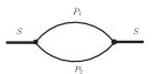
Figure 2: Mass operator of scalar meson $S$.

Using the compositeness condition (42) and the constituents contents of the scalar mesons, one can get the expressions of the coupling constants as

$$\frac{1}{g^{2}_{{}_{a_{0}^{+}}}} = \Sigma_{a_{0}^{+}}^{\prime}(m_{a_{0}}^{2};m_{K^{+}}^{2},m_{K^{0}}^{2})$$

$$\frac{1}{g^{2}_{{}_{a_{0}^{0}}}} = \frac{1}{2}[\Sigma_{a_{0}^{0}}^{\prime}(m_{a_{0}}^{2};m_{K^{+}}^{2},m_{K^{+}}^{2})+\Sigma_{a_{0}^{0}}^{\prime}(m_{a_{0}}^{2};m_{K^{0}}^{2},m_{K^{0}}^{2})]$$

$$\frac{1}{g^{2}_{{}_{K_{0}^{\ast+}}}} = \Sigma_{K_{0}^{\ast+}}^{\prime}(m_{K_{0}^{\ast}}^{2};m_{K^{+}}^{2},m_{\eta}^{2})$$

$$\frac{1}{g^{2}_{{}_{K_{0}^{\ast 0}}}} = \Sigma_{K_{0}^{\ast 0}}^{\prime}(m_{K_{0}^{\ast}}^{2};m_{K^{0}}^{2},m_{\eta}^{2})$$

$$\frac{1}{g^{2}_{{}_{f_{0}}}} = (\frac{\cos\theta_{S}}{\sqrt{6}}+\frac{\sin\theta_{S}}{\sqrt{3}})^{2}[\Sigma_{f_{0}}^{\prime}(m_{f_{0}}^{2};m_{K^{+}}^{2},m_{K^{+}}^{2})+\Sigma_{f_{0}}^{\prime}(m_{f_{0}}^{2};m_{K^{0}}^{2},m_{K^{0}}^{2})]$$

$$+(\frac{\sin\theta_{S}}{\sqrt{3}}-\frac{2\cos\theta_{S}}{\sqrt{6}})^{2}\Sigma_{f_{0}}^{\prime}(m_{f_{0}}^{2};m_{\eta}^{2},m_{\eta}^{2})$$

$$\frac{1}{g^{2}_{{}_{\sigma}}} = (-\frac{\sin\theta_{S}}{\sqrt{6}}+\frac{\cos\theta_{S}}{\sqrt{3}})^{2}[\Sigma_{\sigma}^{\prime}(m_{\sigma}^{2};m_{K^{+}}^{2},m_{K^{+}}^{2})+\Sigma_{\sigma}^{\prime}(m_{\sigma}^{2};m_{K^{0}}^{2},m_{K^{0}}^{2})]$$ (43)

$$+(\frac{\cos\theta_{S}}{\sqrt{3}}+\frac{2\sin\theta_{S}}{\sqrt{6}})^{2}\Sigma_{\sigma}^{\prime}(m_{\sigma}^{2};m_{\eta}^{2},m_{\eta}^{2})$$

The mass operator $\Sigma_{S}^{\prime}(m_{S}^{2};M_{1}^{2},M_{2}^{2})$ can be calculated by evaluating the standard loop integral. From the diagram shown in Fig. 2, in the local interaction case we have

$$\Sigma_{S}^{{\rm LC}~{}\prime}(m_{S}^{2};M_{1}^{2},M_{2}^{2}) = \frac{1}{16\pi^{2}m_{S}^{2}}\Big{\{}\frac{M_{1}^{2}-M_{2}^{2}}{m_{S}^{2}}\ln\frac{M_{1}}{M_{2}}-1$$ (44)

$$\;\;\;\;\;\;\;\;\;\;\;\;\;\;\;\;\;+\frac{m_{S}^{2}(M_{1}^{2}+M_{2}^{2})-(M_{1}^{2}-M_{2}^{2})^{2}}{m_{S}^{2}\sqrt{-\lambda}}\sum_{\pm}\arctan\frac{z_{\pm}}{\sqrt{-\lambda}}\Big{\}}$$

where

$$z_{\pm} = m_{S}^{2}\pm(M_{1}^{2}-M_{2}^{2})$$

$$\lambda \doteq \lambda(m_{S}^{2},M_{1}^{2},M_{2}^{2})$$ (45)

with $\lambda$ as the K$\ddot{a}$llen function. And similarly, for the nonlocal interaction case, the standard evaluation leads to

$$\Sigma_{S}^{{\rm NL}~{}\prime}(m_{S}^{2};M_{1}^{2},M_{2}^{2}) = \frac{1}{16\pi^{2}}\int_{0}^{\infty}\int_{0}^{\infty}d\alpha d\beta\frac{P_{S}}{(1+\alpha+\beta)^{3}}[\frac{d}{dz_{m}}\tilde{\Phi}^{2}(z_{m})]$$ (46)

where

$$P_{S} = \omega_{1}^{2}\alpha+\omega_{2}^{2}\beta+\alpha\beta$$

$$z_{m} = \frac{P_{S}}{1+\alpha+\beta}m_{S}^{2}-\alpha M_{1}^{2}-\beta M_{2}^{2}$$ (47)

It should be noted that the expression (46) is independent of the explicit form of $\tilde{\Phi}$. And in the derivation of (46) we have applied the Laplace Transform

$$F(s) = \int_{0}^{\infty}f(s)e^{-sx}dx;~{}~{}~{}~{}~{}~{}{\rm for~{}Re}s>0$$ (48)

Up to now, the numerical results of the coupling constants $g_{a_{0}^{+}},g_{a_{0}^{0}},g_{K_{0}^{\ast+}}$ and $g_{K_{0}^{\ast 0}}$ can be yielded by inputting the physical masses of the relevant mesons. But the coupling constants $g_{f_{0}}$ and $g_{\sigma}$ can not be got without determining the mixing angle. In the following, we will not discuss the coupling constant $g_{\sigma}$ because of the large uncertainty of the sigma meson mass which should be used in the compositeness condition to determine the coupling constant $g_{\sigma}$. For other scalar mesons, the explicitly input masses are Amsler:2008zz (we adopt the central values of the scalar meson masses)

$$m_{a_{0}} = 985.1~{}{\rm MeV};~{}~{}~{}~{}~{}~{}~{}~{}~{}M_{K_{0}^{\ast}}=672~{}{\rm MeV};~{}~{}~{}~{}~{}~{}~{}~{}~{}~{}m_{f_{0}}=980~{}{\rm MeV}$$

$$m_{K^{+}} = 493.677~{}{\rm MeV};~{}~{}~{}~{}~{}~{}m_{K^{0}}=497.648~{}{\rm MeV};~{}~{}~{}~{}~{}~{}m_{\eta}=547.51~{}{\rm MeV}$$ (49)

With these numerical values, we get the following numerical results for the local interaction coupling constants

$$g_{{}_{a_{0}^{+}}}^{\rm LC} = 3.554~{}{\rm GeV}\;\;;\;\;\;\;g_{{}_{a_{0}^{0}}}^{\rm LC}=3.169~{}{\rm GeV}\;\;;\;\;\;\;g_{{}_{K_{0}^{\ast+}}}^{\rm LC}=12.99~{}{\rm GeV}\;\;;\;\;\;\;g_{{}_{K_{0}^{\ast 0}}}^{\rm LC}=13.06~{}{\rm GeV}$$

$$\frac{1}{g^{\rm LC~{}2}_{{}_{f_{0}}}} = 0.1194\times(-\frac{\sin\theta_{S}}{\sqrt{6}}+\frac{\cos\theta_{S}}{\sqrt{3}})^{2}+0.0117\times(\frac{\cos\theta_{S}}{\sqrt{3}}+\frac{2\sin\theta_{S}}{\sqrt{6}})^{2}$$ (50)

In the following, we will fix the coupling constant $g_{f_{0}}$ and mixing angle $\theta_{S}$ using the two-photon decay of $f_{0}$. The two-photon decay of $f_{0}\to 2\gamma$ has been studied in the hadronic molecular model in Refs. Giacosa:2007bs ; Branz:2007xp ; Branz:2008ha . In the local interaction case, one should consider the diagrams shown in Fig. 3. And, even in the nonlocal interaction case, only including these diagrams is enough since, to our experiences, the contributions from diagrams with photon emerges from the nonlocal vertex are negligible.

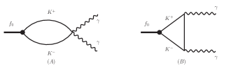
Figure 3: Diagrams contribute to the decays of $f_{0}\to 2\gamma$.

Generally, the width for decay $f_{0}\to 2\gamma$ can be expressed as

$$\Gamma(S\to 2\gamma) = 16\pi\alpha_{\rm em}^{2}\tilde{g}_{{}_{f_{0}}}^{2}G^{2}(m_{S}^{2})m_{S}^{3};$$ (51)

And, because there are only charged kaon mesons in the loop, $\tilde{g}_{{}_{f_{0}}}$ relates to the coupling constant $g_{{}_{f_{0}}}$ via relations

$$\tilde{g}_{{}_{f_{0}}} = g_{{}_{f_{0}}}(\frac{\cos\theta}{\sqrt{6}}+\frac{\sin\theta}{\sqrt{3}})$$ (52)

For the local interaction case, after standard calculation we get

$$G^{\rm LC}(m_{f_{0}}^{2}) = \frac{1}{16\pi^{2}}\int_{0}^{1}dx_{1}\int_{0}^{1-x_{1}}dx_{2}\frac{x_{1}x_{2}}{-x_{1}x_{2}m_{f_{0}}^{2}+m_{K}^{2}}$$ (53)

And for the nonlocal interaction, we get

$$G^{\rm NL}(m_{f_{0}}^{2}) = \frac{1}{16\pi^{2}}\frac{1}{\Lambda_{S}^{2}}\int_{0}^{\infty}d\alpha_{1}d\alpha_{2}d\alpha_{3}\frac{1}{(1+\sum_{i=1}^{3}\alpha_{i})^{4}}(\frac{1}{2}+\alpha_{1})(\frac{1}{2}+\alpha_{2})\Phi(z_{R})$$ (54)

with

$$z_{R} = -\frac{1}{1+\sum_{i=1}^{3}\alpha_{i}}(\frac{1}{2}+\alpha_{2}+\alpha_{3})(\frac{1}{2}+\alpha_{2})m_{f_{0}}^{2}+(\frac{1}{4}+\alpha_{2})m_{f_{0}}^{2}-\sum_{i=1}^{3}\alpha_{i}m_{K}^{2}$$ (55)

Using the average data quoted by PDG Amsler:2008zz

$$\Gamma(f_{0}\to 2\gamma) = 0.29^{+0.07}_{-0.09}{~{}\rm KeV}$$ (56)

and the expression (53), we have the numerical results of the coupling constant $\tilde{g}_{f_{0}}$ as

$$\tilde{g}_{f_{0}}^{\rm LC} = 2.878~{}{\rm GeV};$$

$$\tilde{g}_{f_{0}}^{\rm NL} = 2.941-2.915~{}{\rm GeV};\;\;\;{\rm for}\;\;\Lambda_{S}=3.0-4.0{~{}\rm GeV}$$ (57)

which leads to

$$g_{f_{0}}^{\rm LC} = 4.175{~{}\rm GeV};~{}~{}~{}~{}~{}~{}{\rm for~{}~{}}\theta_{S}=42^{\circ}$$

$$g^{\rm LC}_{f_{0}} = 4.182{~{}\rm GeV};~{}~{}~{}~{}~{}~{}{\rm for~{}~{}}\theta_{S}=68^{\circ}$$ (58)

In principle, with the help of the decay of $\sigma\to 2\gamma$ one can determine the exact value of $\theta_{S}$ if this model can explain all the data well. But, as we mentioned above, we will not study the physics of $\sigma$ meson because of its large mass uncertainty, so that at present we will adopt $\theta_{S}=68^{\circ}$. We would like to point out that our final results do not depend on the choice of $\theta_{S}$ closely, since the two angles lead to the same effective $f_{0}KK$ coupling constant and the $\eta\eta$ component plays negligible roles in the quantities we calculated.

Using the same method, in the nonlocal interaction case, one can also determine the effective coupling constants $g_{{}_{S}}$. In this case, since the coupling constants are functions of $\Lambda_{S}$, one should determine the magnitude of $\Lambda_{S}$ at first. Our principle is that the effective coupling constants should be stable against $\Lambda_{S}$. With this criterion in mind, and running $\Lambda_{S}$ from $1.0~{}$GeV to $10.0~{}$GeV, we find the physical region of $\Lambda_{S}$ should be $3.0-4.0~{}$GeV. We list the numerical results of $g_{{}_{S}}$ in Table.1 and compare them with that from the local interaction case and other literature.

Table 1: Numerical results of the coupling constants $g_{{}_{S}}$ (in unit of GeV). The range of our results is due to the variation of $\Lambda_{S}$ from $3.0-4.0~{}$GeV.

	$g_{a_{0}^{\pm}}$	$g_{a_{0}^{0}}$	$g_{K_{0}^{\ast\pm}}$	$g_{K_{0}^{\ast 0}}$	$g_{f_{0}}$	$\theta_{S}$
Our results (NL)	$3.591\sim 3.577$	$3.252-3.227$	$14.13-13.73$	$13.23-13.81$	$4.230\sim 4.210$	$42^{\circ}$
					$4.237-4.217$	$68^{\circ}$
Our results (LC)	$3.554$	$3.169$	$12.99$	$13.06$	$4.175$	$42^{\circ}$
					$4.182$	$68^{\circ}$
Ref. Branz:2007xp					$3.09$
Ref. Branz:2008ha	$3.61$ (NL)	$3.61$ (NL)			$3.06$ (NL)
	$3.45$ (LC)	$3.45$ (LC)			$2.87$ (LC)
Ref. Napsuciale:2004au					$3.27\pm 0.99$

In this table we find in the physical region of $\Lambda_{S}$ all the coupling constants calculated in the nonlocal interaction case agree with that yielded in the local interaction case. However, compared with Ref. Branz:2007xp , one find that our result for $g_{{}_{f_{0}}}$ is much larger. This is because, in the present construction, in addition to the $KK$ constituents, $f_{0}$ also consists of $\eta\eta$ component so there is the mixing angle $\theta_{S}$. When the mixing angle $\theta_{S}$ is included our effective coupling constant $g_{{}_{f_{0}KK}}$ agrees with that given in the literature. This is one of the typical properties of the present work. Concerning the typical property that numerical values of the coupling constants yielded from the nonlocal interaction case agree with that from the local interaction case, in the following calculation, we will adopt the local interaction vertex.

At last we would like to mention that, because of the $K\bar{K}$ components in $f_{0}$ and $a_{0}^{0}$, there is $a_{0}^{0}-f_{0}$ mixing in the hadronic molecular model. In the present work we will not study the mixing effect of these two mesons. For persons who interest in this topic please see Refs. Branz:2008ha ; Wu:2007jh ; Wu:2008hx and the relevant references therein.

II.3 The Leptonic Decays of the Scalar Mesons

Next, we will calculate the scalar meson leptonic decay widths in the molecular picture. It is well known that, for a pseudoscalar meson, for example $\pi^{+}$, the leptonic decay constant $f_{\pi}$ is defined by

$$\langle|\bar{u}\gamma_{\mu}\gamma_{5}d|\pi^{-}(p_{\pi})\rangle = -if_{\pi}p_{\pi}^{\mu}$$ (59)

And since leptons are free from strong interaction, one can express the width of the pion weak decay $\pi^{-}\to l\bar{\nu}_{l}$ in terms of the leptonic decay constant $f_{\pi}$ using naive factorization. Comparing with the data, one can extract the numerical value of $f_{\pi}$. On the other hand, if the wave function of pion is known, we can also calculate this quantity by the standard loop integral. For our present problem, the scalar mesons are interpreted as hadronic molecules and the coupling constant between the scalar meson and its constituents is determined by the compositeness condition. So that we can calculate the leptonic decay constants of scalar mesons via the standard loop integral. At the meson level, we define the leptonic decay constant of the scalar meson via

$$\langle S(p)|P_{1}\partial^{{}^{{}^{\leftrightarrow}}}_{\mu}P_{2}|0\rangle = ip_{\mu}f_{s}$$ (60)

where $p_{\mu}$ is the momentum of scalar meson and $P_{1}$ and $P_{2}$ are the two constituents of scalar meson $S$. To calculated this quantity, one should concern the the Feynman diagram depicted in Fig. 4.

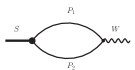
Figure 4: Diagram relates to the leptonic decay constant of the charged scalar meson.

The coupling constants between the weak gauge bosons and pseudoscalar mesons can be yielded by gauging the nonlinear sigma model and relating the flavor symmetry of the nonlinear sigma model to the flavor symmetry of QCD. The relevant terms are HerreraSiklody:1996pm

$${\cal L}_{\rm nl\sigma}^{\rm gauged} = \frac{F_{\pi}^{2}}{4}{\rm Tr}[D_{\mu}U(D_{\mu}U^{\dagger})+\chi^{\dagger}U+U^{\dagger}\chi]$$ (61)

where $\chi=2BM$ with $B$ as a constant relating to the quark condensation and $M={\rm diag}(m_{u},m_{d},m_{s})$ as the quark mass matrix. The field $U(x)$ is expressed in terms of pseudoscalar fields as

$$U(x) = \exp(i\phi(x)/F_{\pi})$$

$$\phi(x) = \left(\begin{array}[]{ccc}\pi^{0}+\frac{1}{\sqrt{3}}\eta&\sqrt{2}\pi^{+}&\sqrt{2}K^{+}\\ \sqrt{2}\pi^{-}&-\pi^{0}+\frac{1}{\sqrt{3}}\eta&\sqrt{2}K^{0}\\ \sqrt{2}K^{-}&\sqrt{2}\bar{K}^{0}&-\frac{2}{\sqrt{3}}\eta\\ \end{array}\right)$$ (65)

where $F_{\pi}$ is the pion leptonic decay constant with the value $F_{\pi}=92.5{~{}\rm MeV}$. Under $SU(3)_{L}\times SU(3)_{R}$ chiral transformation meson matrix $U(x)$ transforms as

$$U(x) \rightarrow g_{R}U(x)g_{L}^{\dagger}$$ (66)

The covariant derivative is defined as

$$D_{\mu}U = \partial_{\mu}U-iA_{R;\mu}U+iUA_{L;\mu}$$ (67)

$A_{L;\mu}$ and $A_{R;\mu}$ are the gauge fields corresponding to the gauged left- and right-handed chiral symmetry, respectively.

By matching the chiral symmetry of QCD and the transformation of the field $U(x)$ one can express these gauge fields in terms of the electroweak gauge bosons as Harada:1995sj

$$A_{R;\mu} = -eQA_{\mu}-g\frac{\sin^{2}\theta_{W}}{\cos\theta_{W}}QZ_{\mu}$$

$$A_{L;\mu} = -eQA_{\mu}+gQ_{Z}Z_{\mu}+\frac{g}{\sqrt{2}}(W_{\mu}^{+}Q_{W}+W_{\mu}^{-}Q_{W}^{\dagger})$$ (68)

where $Q$ is the charge matrix of quarks and in the three flavor case $Q={\rm diag}(2/3,-1/3,-1/3)$ and $e=g\sin\theta_{W}$. The matrices $Q_{W}$ and $Q_{Z}$ are defined as

$$Q_{W} = \left(\begin{array}[]{ccc}0&V_{ud}&V_{us}\\ 0&0&0\\ 0&0&0\\ \end{array}\right);\;\;\;\;\;\;\;Q_{Z}=\frac{1}{\cos\theta}\left(\begin{array}[]{ccc}1/2&0&0\\ 0&-1/2&0\\ 0&0&-1/2\\ \end{array}\right)-\frac{\sin^{2}\theta_{W}}{\cos\theta_{W}}Q$$ (75)

where $V_{ud}$ and $V_{us}$ are the appropriate Cabibbo-Kobayashi-Maskawa matrix elements. And $g$ is the coupling constant of the $SU(2)_{L}$ weak gauge group in the standard model and at the lowest order perturbation theory it is determined by the Fermi constant and the W boson mass via the relation Amsler:2008zz

$$G_{F} = \sqrt{2}\frac{g^{2}}{8m_{W}^{2}}=1.16637(1)\times 10^{-5}{\rm GeV}^{-2}$$ (76)

Explicitly, one can get the following $WPP$ interaction Lagrangian

$${\cal L}_{W}^{W} = -\frac{ig}{4\sqrt{2}}W^{+}_{\mu}\Big{[}2V_{ud}K^{0}\partial^{{}^{{}^{\leftrightarrow}}}_{\mu}K^{-}-\sqrt{6}V_{us}\eta\partial^{{}^{{}^{\leftrightarrow}}}_{\mu}K^{-}\Big{]}$$ (77)

As an example, let us consider the decay of $a_{0}^{-}(980)\to l\bar{\nu}_{l}$. Its matrix element, on the one hand, can be expressed in terms of the leptonic decay constant $f_{a_{0}^{+}}$, and on the other hand, can be calculated directly from the relevant Feynman diagram in terms of the coupling constant $g_{a_{0}^{+}}$, so that $f_{a_{0}^{+}}$ can be expressed as a function of the coupling constant $g_{a_{0}^{+}}$. In this sense the numerical value of $f_{a_{0}^{+}}$ is calculable in the molecular model.

Consider the following effective Hamiltonion

$$H_{\rm eff} = \sqrt{2}iG_{F}V_{ud}[K^{0}\partial^{{}^{{}^{\leftrightarrow}}}_{\mu}K^{-}][\bar{l}\gamma_{\mu}P_{L}\nu_{l}]$$ (78)

on the one hand, the relevant matrix element, with the help of ”naive factorization”, can be written as

$$iM(a_{0}^{-}\to l\bar{\nu}_{l}) = -\sqrt{2}iG_{F}V_{ud}\langle l,\bar{\nu}_{l}|[K^{0}\partial^{{}^{{}^{\leftrightarrow}}}_{\mu}K^{-}][\bar{l}\gamma_{\mu}P_{L}\nu_{l}]|a_{0}^{-}\rangle$$ (79)

$$= \sqrt{2}G_{F}V_{ud}p_{a_{0}^{-}}^{\mu}f_{a_{0}^{-}}\bar{u}(p_{\mu})\gamma_{\mu}P_{L}v(p_{\nu_{\mu}})$$

On the other hand, this matrix element can be expressed in terms of the coupling constant $g_{a_{0}^{+}}$ and standard loop integral as

$$iM(a_{0}^{-}\to l\bar{\nu}_{l}) = -\sqrt{2}G_{F}V_{ud}\bar{u}(p_{\mu})\gamma_{\mu}P_{L}v(p_{\nu_{\mu}})$$ (80)

$$\times g_{a_{0}^{+}}\int\frac{d^{4}k}{(2\pi)^{4}}\frac{1}{k^{2}-m_{K^{0}}^{2}}\frac{1}{(k+p)^{2}-m_{K^{+}}^{2}}(2k+p_{a_{0}^{-}})_{\mu}$$

Comparing (79) and (80) and after some calculations, one gets the leptonic decay constant of $a_{0}$ as

$$f_{a_{0}^{-}} = g_{a_{0}^{+}}I(m_{a_{0}}^{2},m_{K^{0}}^{2},m_{K^{+}}^{2})$$ (81)

where

$$I(m_{a_{0}}^{2},m_{K^{0}}^{2},m_{K^{+}}^{2}) = \int_{0}^{1}dx(1-2x)\ln\Big{[}\frac{(1-x)m_{K^{0}}^{2}+xm_{K^{+}}^{2}-x(1-x)m_{a_{0}}^{2}}{\mu^{2}}\Big{]}$$ (82)

where $\mu$ is the dimensional parameter introduced in dimensional regularization. It should be noted that, in this expression, the term $(1-2x)\ln\mu^{2}$ vanishes after the Feynman parameter integral. In this sense the the expression (82) is scale independent. With the Eqs. (81,82) we get the numerical result of the leptonic decay constant $f_{a_{0}^{+}}$ for scalar meson $a_{0}^{+}$ as

$$f_{a_{0}^{+}} = g_{a_{0}^{+}}I_{L}(m_{a_{0}}^{2},m_{K^{+}}^{2},m_{K^{0}}^{2})=0.1530~{}{\rm MeV}$$ (83)

Similarly, one can get the leptonic decay constant for $K_{0}^{\ast+}$ as

$$f_{K_{0}^{\ast+}} = g_{K_{0}^{\ast+}}I_{L}(m_{K_{0}^{\ast}}^{2},m_{K^{+}}^{2},m_{\eta}^{2})=3.463~{}{\rm MeV}$$ (84)

For $K_{0}^{\ast 0}$ meson, one can also define its leptonic decay constant as (60) and express $f_{K_{0}^{\ast 0}}$ as (81). The numerical calculation yields

$$f_{K_{0}^{\ast 0}} = g_{K_{0}^{\ast 0}}I_{L}(m_{K_{0}^{\ast}}^{2},m_{K^{0}}^{2},m_{\eta}^{2})=3.208~{}{\rm MeV}$$ (85)

From this result one can see that the isospin violating effect is important for the study of $K_{0}^{\ast}$ mesons in the molecular model.

We would like to mention that, in contrast to the quark model where the leptonic decay constants of neutral mesons are identified with their charged partners, the leptonic decay constants of neutral molecular scalar mesons $f_{0}$ and $a_{0}^{0}$ are zero since, equation (82) vanishes in case of $M_{1}=M_{2}$. Physically, this is because the weak interaction (and the electromagnetic interaction) is mediated by vector current of pseudoscalar mesons.

With the help of leptonic decay constants calculated above, we can calculate the leptonic decay of the charged scalar mesons. In terms of the leptonic decay constants, one can express the partial width for decay $a_{0}^{-}\to l\bar{\nu}_{l}$ as

$$\Gamma(a_{0}^{-}\to l\bar{\nu}_{l}) = \frac{G_{F}^{2}|V_{ud}|^{2}}{8\pi}f_{{}_{a_{0}^{+}}}^{2}m_{a_{0}}m_{l}^{2}\Big{(}1-\frac{m_{l}^{2}}{m_{a_{0}}^{2}}\Big{)}^{2}$$ (86)

Along the same derivation, the leptonic decay width of $K_{0}^{\ast-}\to l\bar{\nu}_{l}$ can be expressed as

$$\Gamma(K_{0}^{\ast-}\to l\bar{\nu}_{l}) = \frac{6G_{F}^{2}|V_{us}|^{2}}{32\pi}f_{{}_{K_{0}^{\ast}}}^{2}m_{K_{0}^{\ast}}m_{l}^{2}\Big{(}1-\frac{m_{l}^{2}}{m_{K_{0}^{\ast}}^{2}}\Big{)}^{2}$$ (87)

The numerical results are found to be

$$\Gamma(a^{-}\to e^{-}\bar{\nu}_{e}) = 3.091\times 10^{-20}{\rm~{}KeV}~{}~{};~{}~{}~{}~{}~{}~{}\Gamma(a^{-}\to\mu^{-}\bar{\nu}_{\mu})=1.306\times 10^{-15}{\rm~{}KeV}$$

$$\Gamma(K_{0}^{\ast-}\to e^{-}\bar{\nu}_{e}) = 1.620\times 10^{-17}{\rm~{}KeV}~{}~{};~{}~{}~{}~{}~{}~{}\Gamma(K_{0}^{\ast-}\to\mu^{-}\bar{\nu}_{\mu})=6.755\times 10^{-13}{\rm~{}KeV}$$ (88)

From these numerical results we conclude that, in the hadronic molecular interpretation, it is difficult to search for the leptonic decays of the charged scalar mesons in the near future. Or inversely, if the observed leptonic decay widths of scalar mesons are much larger than the present results, the hadronic molecular interpretation is suspectable.

III Strong Decays of Light Scalar Mesons

In this section, based on the hadronic molecular explanation, we will study the strong decays of the light scalar mesons with masses below 1.0 GeV. Explicitly, we will study the scalar meson to two-pseudoscalar meson decays, i.e., the decays of $a_{0}^{+}\to\eta\pi^{+},a_{0}^{0}\to\eta\pi^{0},K_{0}^{\ast+}\to K\pi,K_{0}^{\ast 0}\to K\pi$ and $f_{0}\to\pi\pi$. These processes are important since they are the dominant channels for the relevant scalar mesons Amsler:2008zz . To study these decays, one should consider the two kinds of Feynman diagrams depicted in Fig. 5. Diagram (A) is from the four-pseudoscalar meson vertex, while diagram (B) arises from the final state interaction.

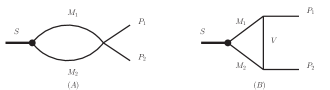
Figure 5: Feynman diagrams contributing to the strong decay of $S\to P_{1}P_{2}$ ($M_{i}$ denotes the constituent meson, $P_{i}$ denotes the final pseudoscalar meson and $V$ denotes the relevant vector meson).

In the explicit calculation, we need the four-pseudoscalar interaction vertices which give diagram (A) of Fig. 5. Here we only consider the terms from the leading order chiral perturbation theory with the explicit chiral symmetry breaking terms Gasser:1983yg ; Gasser:1984gg

$${\cal L}^{\mathcal{O}(2)} = \frac{F_{\pi}^{2}}{4}{\rm Tr}[\partial_{\mu}U(\partial_{\mu}U^{\dagger})+\chi^{\dagger}U+U^{\dagger}\chi]$$ (89)

$$= \frac{1}{24F_{\pi}^{2}}$$

$$\times\Big{\{}\Big{[}4(\pi^{-}\partial^{{}^{{}^{\leftrightarrow}}}_{\mu}\bar{K}^{0})(K^{0}\partial^{{}^{{}^{\leftrightarrow}}}_{\mu}\pi^{+})+4(K^{0}\partial^{{}^{{}^{\leftrightarrow}}}_{\mu}\bar{K}^{0})(\pi^{-}\partial^{{}^{{}^{\leftrightarrow}}}_{\mu}\pi^{+})+4(m_{K}^{2}+m_{\pi}^{2})K^{0}\bar{K}^{0}\pi^{+}\pi^{-}\Big{]}$$

$$\;\;\;+\Big{[}4(\pi^{-}\partial^{{}^{{}^{\leftrightarrow}}}_{\mu}K^{+})(K^{-}\partial^{{}^{{}^{\leftrightarrow}}}_{\mu}\pi^{+})+4(K^{-}\partial^{{}^{{}^{\leftrightarrow}}}_{\mu}K^{+})(\pi^{-}\partial^{{}^{{}^{\leftrightarrow}}}_{\mu}\pi^{+})+4(m_{K}^{2}+m_{\pi}^{2})K^{+}K^{-}\pi^{+}\pi^{-}\Big{]}$$

$$\;\;\;+\Big{[}2\sqrt{3}(\eta\partial^{{}^{{}^{\leftrightarrow}}}_{\mu}K^{0})(\pi^{0}\partial^{{}^{{}^{\leftrightarrow}}}_{\mu}\bar{K}^{0})+2\sqrt{3}(\eta\partial^{{}^{{}^{\leftrightarrow}}}_{\mu}\bar{K}^{0})(\pi^{0}\partial^{{}^{{}^{\leftrightarrow}}}_{\mu}K^{0})+\frac{4}{\sqrt{3}}(m_{K}^{2}-m_{\pi}^{2})K^{0}\bar{K}^{0}\pi^{0}\eta\Big{]}$$

$$\;\;\;+\Big{[}2\sqrt{6}(\eta\partial^{{}^{{}^{\leftrightarrow}}}_{\mu}K^{0})(K^{-}\partial^{{}^{{}^{\leftrightarrow}}}_{\mu}\pi^{+})+2\sqrt{6}(\eta\partial^{{}^{{}^{\leftrightarrow}}}_{\mu}K^{-})(K^{0}\partial^{{}^{{}^{\leftrightarrow}}}_{\mu}\pi^{+})-4\sqrt{\frac{2}{3}}(m_{K}^{2}-m_{\pi}^{2})K^{0}K^{-}\pi^{+}\eta\Big{]}$$

$$\;\;\;+\Big{[}2\sqrt{6}(\eta\partial^{{}^{{}^{\leftrightarrow}}}_{\mu}\bar{K}^{0})(K^{+}\partial^{{}^{{}^{\leftrightarrow}}}_{\mu}\pi^{-})+2\sqrt{6}(\eta\partial^{{}^{{}^{\leftrightarrow}}}_{\mu}K^{+})(\bar{K}^{0}\partial^{{}^{{}^{\leftrightarrow}}}_{\mu}\pi^{-})-4\sqrt{\frac{2}{3}}(m_{K}^{2}-m_{\pi}^{2})K^{+}\bar{K}^{0}\pi^{-}\eta\Big{]}$$

$$\;\;\;+\Big{[}2\sqrt{3}(\eta\partial^{{}^{{}^{\leftrightarrow}}}_{\mu}K^{-})(K^{+}\partial^{{}^{{}^{\leftrightarrow}}}_{\mu}\pi^{0})+2\sqrt{3}(\eta\partial^{{}^{{}^{\leftrightarrow}}}_{\mu}K^{+})(K^{-}\partial^{{}^{{}^{\leftrightarrow}}}_{\mu}\pi^{0})-\frac{4}{\sqrt{3}}(m_{K}^{2}-m_{\pi}^{2})K^{+}K^{-}\pi^{0}\eta\Big{]}$$

$$\;\;\;+4m_{\pi}^{2}\pi^{+}\pi^{-}\eta\eta\Big{\}}+\cdots$$

where only terms will be used in our calculation were written down. And to derive these relations we have used the Gell-Mann-Okubo mass relation

$$4m_{K}^{2} = 3m_{\eta}^{2}+m_{\pi}^{2}$$ (90)

The interaction Lagrangian for vector-pseudoscalar-pseudoscalar meson vertex can be written as

$${\cal L}_{K^{\ast}K\pi} = \frac{ig_{K^{\ast}K\pi}}{\sqrt{2}}K^{\ast~{}{\dagger}}_{\mu}(x)\vec{\tau}\cdot\vec{\pi}(x)\partial_{\mu}^{{}^{{}^{\leftrightarrow}}}K(x)+{\rm H.c}$$

$${\cal L}_{K^{\ast}K\eta} = \frac{ig_{K^{\ast}K\eta}}{\sqrt{2}}K^{\ast~{}{\dagger}}_{\mu}(x)\eta(x)\partial_{\mu}^{{}^{{}^{\leftrightarrow}}}K(x)+{\rm H.c}$$ (91)

where the summation over isospin indices is understood and $A\partial_{\mu}^{{}^{{}^{\leftrightarrow}}}B\equiv A\partial_{\mu}B-B\partial_{\mu}A$. The coupling constant $g_{K^{\ast}K\pi}$ can be fixed from the data for the strong decay width $K^{\ast}\to K\pi$. In particular the strong decay width $\Gamma(K^{\ast}\to K\pi)$ relates to $g_{K^{\ast}K\pi}$ via

$$\Gamma(K^{\ast}\to K\pi) = \frac{g_{K^{\ast}K\pi}^{2}}{6\pi m_{K^{\ast}}^{2}}P_{\pi K^{\ast}}^{3}$$ (92)

where $P_{\pi K^{\ast}}$ is the three-momentum of $\pi$ in the rest frame of $K^{\ast}$. Using the data for the decay width one can deduce $g_{K^{\ast}K\pi}=4.61$ Amsler:2008zz . The coupling constant $g_{K^{\ast}K\eta}$ can be related to the $g_{K^{\ast}K\pi}$ using the unitary symmetry relation

$$g_{K^{\ast}K\eta} = \frac{F_{\pi}\sqrt{3}}{F_{\eta}}g_{K^{\ast}K\pi}=6.14$$ (93)

Generally, the matrix elements corresponding to these two kinds of diagrams can be written as

$$iM^{(A)}(S\to P_{1}P_{2}) = ig_{{}_{S}}g_{{}_{M_{1}M_{2}P_{1}P_{2}}}I^{(A)}(m_{S};M_{1},M_{2};m_{1},m_{2})$$

$$iM^{(B)}(S\to P_{1}P_{2}) = ig_{{}_{S}}g_{{}_{VM_{1}P_{1}}}g_{{}_{VM_{2}P_{2}}}I^{(B)}(m_{S};m_{V};M_{1},M_{2};m_{1},m_{2})$$ (94)

where the notation $m_{i}$ is the mass of the final state, $g_{{}_{M_{1}M_{2}P_{1}P_{2}}}$ is the coupling constant of four-pseudoscalar meson vertex which was taken from the leading order Chiral perturbation theory Gasser:1983yg ; Gasser:1984gg and $g_{{}_{VM_{i}P_{i}}}$ is the coupling constant of vector-pseudoscalar-pseudoscalar meson vertex. The functions $I^{(A)}$ and $I^{(B)}$ can be calculated using the standard technics of loop integral. Concerning the effective Lagrangian (89), we will choose $g_{{}_{M_{1}M_{2}P_{1}P_{2}}}=1/(24F_{\pi}^{2})$.

So we formally write the matrix element of $S\to P_{1}P_{2}$ decay as

$$iM(S\to P_{1}P_{2}) = iM^{(A)}(S\to P_{1}P_{2})+iM^{(B)}(S\to P_{1}P_{2})$$ (95)

The decay width, in terms of $I^{(A)}$ and $I^{(B)}$, can be expressed as

$$\Gamma(S\to P_{1}P_{2}) = \frac{g_{{}_{S}}^{2}}{8\pi m_{S}^{2}}\Big{|}\vec{p}_{cm}(m_{S}^{2};m_{1}^{2},m_{2}^{2})\Big{|}$$ (96)

$$\times\Big{|}g_{{}_{M_{1}M_{2}P_{1}P_{2}}}I^{(A)}(m_{S};M_{1},M_{2};m_{1},m_{2})$$

$$\;\;\;\;+g_{{}_{VM_{1}P_{1}}}g_{{}_{VM_{2}P_{2}}}I^{(B)}(m_{S};M_{1},M_{2};m_{V};m_{1},m_{2})\Big{|}^{2}$$

where $\Big{|}\vec{p}_{cm}(m_{S}^{2};m_{1}^{2},m_{2}^{2})\Big{|}=\frac{1}{2m_{S}}\lambda(m_{S}^{2};m_{1}^{2},m_{2}^{2})$ with $\lambda$ as the K$\ddot{a}$llen function.

Now, we will calculate the width for strong decay $a_{0}^{+}\to\pi^{+}\eta$. At first, let’s consider the function $I^{(A)}$. From the interaction Lagrangian given in Eq. (89), one can see that the four-pseudoscalar-meson vertex consists of two parts: the part includes derivative and the other part without derivative. So that we can formally do the decomposition

$$I^{(A)}(m_{a_{0}};m_{K^{+}},m_{K^{0}};m_{\eta},m_{\pi^{+}}) = g_{P_{1}P_{2}P_{3}P_{4}}^{D}I^{(A)}_{D}(m_{a_{0}};m_{K^{+}},m_{K^{0}};m_{\eta},m_{\pi^{+}})$$ (97)

$$+g_{P_{1}P_{2}P_{3}P_{4}}^{ND}I^{(A)}_{ND}(m_{a_{0}};m_{K^{+}},m_{K^{0}};m_{\eta},m_{\pi^{+}})$$

where the upper indices $D$ and $ND$ denote the contributions from Lagrangian with derivative and without derivative terms, respectively. After explicit calculation, we get

$$I_{D}^{(A)}(m_{a_{0}};m_{K^{+}},m_{K^{0}};m_{\eta},m_{\pi^{+}}) = \int\frac{d^{4}k}{(2\pi)^{4}}\mathcal{F}(k^{2})\frac{i}{k^{2}-m_{K}^{2}}\frac{i}{(k+p)^{2}-m_{K^{0}}^{2}}$$

$$\;\;\;\;\;\;\;\;\;\;\;\;\times\Big{[}[(k+p)+p_{1}]\cdot(k-p_{2})+(p_{1}-k)\cdot[-p_{1}-(k+p)]\Big{]}$$

$$I_{ND}^{(A)}(m_{a_{0}};m_{K^{+}},m_{K^{0}};m_{\eta},m_{\pi^{+}}) = \int\frac{d^{4}k}{(2\pi)^{4}}\mathcal{F}(k^{2})\frac{i}{k^{2}-m_{K}^{2}}\frac{i}{(k+p)^{2}-m_{K^{0}}^{2}}$$ (99)

where $p$ is the momentum of the incoming $a_{0}^{+}$ meson, and $p_{1}$ and $p_{2}$ are momentum of the outgoing $\eta$ and $\pi^{+}$, respectively. Since the momentum integral is divergent, the form factor ${\cal F}(q^{2})$ was introduced to suppress the divergence. Explicitly, the momentum-dependence of the form factor is

$${\cal F}(q^{2}) = \Big{(}\frac{\Lambda^{2}-m_{K}^{2}}{\Lambda^{2}-q^{2}}\Big{)}^{n}$$ (100)

where $n=1,2$ correspond to the monopole and dipole forms, respectively Machleidt:1987hj . Through out the following calculation we will select the dipole form since the above integral is quadratically divergent, i.e., $n=2$. For the parameter $\Lambda$, since we only include the diagrams with the exchanged mass up to $m_{{}_{K^{\ast}}}$, we will take the typical value $\Lambda=1.0~{}$GeV. In Appendix. A, we express $I_{D}^{(A)}$ and $I_{ND}^{(A)}$ in terms of the standard n-point scalar and tensor integrals.

For diagram (B) we have

$$I^{(B)}(m_{a_{0}};m_{K^{+}},m_{K^{0}};m_{\eta},m_{\pi^{+}}) = \int\frac{d^{4}k}{(2\pi)^{4}}{\cal F}(k^{2})\frac{i}{(k-p_{1})^{2}-m_{K}^{2}}\frac{i}{(k+p_{2})^{2}-m_{K^{0}}^{2}}\frac{-i}{k^{2}-m_{K^{\ast}}^{2}}$$ (101)

$$\times(2p_{1}-k)_{\mu}[g_{\mu\nu}-\frac{k_{\mu}k_{\nu}}{m_{K^{\ast}}^{2}}](k+2p_{2})_{\nu}$$

which is also expressed in terms of the standard n-point scalar and tensor integrals in Appendix. A.

Substituting the relevant masses and coupling constants and with the help of the software package LoopTools Hahn:1998yk , we get the width for the strong decay $a_{0}^{+}\to\pi^{+}\eta$ as

$$\Gamma(a_{0}^{+}\to\pi^{+}\eta) = 58.81{~{}\rm MeV}$$ (102)

Along the same method, one can get the following decay width

$$\Gamma(a_{0}^{0}\to\pi^{0}\eta) = 59.21{~{}\rm MeV}$$ (103)

Similarly, for other strong decay widths we have

$$\Gamma(K_{0}^{\ast+}\to K^{0}\pi^{+}) = 11.06{~{}\rm MeV}$$ (104)

$$\Gamma(K_{0}^{\ast 0}\to K^{-}\pi^{+}) = 12.37{~{}\rm MeV}$$ (105)

$$\Gamma(f_{0}\to\pi^{+}\pi^{-}) = 30.65{~{}\rm MeV}$$ (106)

It should be noted that the analytic forms of diagram (A) in Fig. 5 for these three processes are different from that of $a_{0}\to\eta\pi$ decay we listed in Appendix. A. For simplicity, we will not write it down explicitly.

With the help of the isospin relation, we get the following decay widths

$$\Gamma(K_{0}^{\ast+}\to K\pi) = \Gamma(K_{0}^{\ast+}\to K^{+}\pi^{0})+\Gamma(K_{0}^{\ast+}\to K^{0}\pi^{+})=\frac{3}{2}\Gamma(K_{0}^{\ast+}\to K^{0}\pi^{+})=16.59{~{}\rm MeV}$$

$$\Gamma(K_{0}^{\ast 0}\to K\pi) = \Gamma(K_{0}^{\ast 0}\to K^{+}\pi^{-})+\Gamma(K_{0}^{\ast 0}\to K^{0}\pi^{0})=\frac{3}{2}\Gamma(K_{0}^{\ast 0}\to K^{+}\pi^{-})=18.56{~{}\rm MeV}$$

$$\Gamma(f_{0}\to\pi\pi) = \Gamma(f_{0}\to\pi^{+}\pi^{-})+\frac{1}{2}\Gamma(f_{0}\to\pi^{0}\pi^{0})=45.98{~{}\rm MeV}$$ (107)

We summarize our results and compare them with that given in the literature in Table. 2. From this table we see our results for $\Gamma(f_{0}\to\pi\pi)$ and $\Gamma(a_{0}\to\eta\pi)$ agree with that of Ref. Branz:2008ha , and the tiny differences can be understood by concerning that the scalar-pseudoscalar-pseudoscalar vertices used in the present work are local one but that in Ref. Branz:2008ha are nonlocal. This indirectly indicates that the scale $\Lambda=1.0~{}$GeV we chose is reasonable. For the $f_{0}\to\pi\pi$ decay, our result is consistent with that from both the $q\bar{q}$ and tetraquark interpretations and all the results are consistent with that given in PDG. For the $a_{0}\to\eta\pi$ decays, the results from both the hadronic molecular interpretation and tetraquark interpretation are consistent with the data but hadronic interpretation leads to a smaller result than the tetraquark interpretation. At last, let us turn to the results of $K_{0}^{\ast}$ decays. One can see that our result is much smaller than the data and other theoretical approaches. In fact, concerning our yielded result is based on the central value of $K_{0}^{\ast}$ mass, $m_{K_{0}^{\ast}}=672~{}$MeV Amsler:2008zz , we varied $m_{K_{0}^{\ast}}$ up to $1.0~{}$GeV as a check and it is found that $\Gamma(K_{0}^{\ast}\to K\pi)<70~{}$MeV which is still much smaller than the data and other approaches. In this sense, it is difficult to arrange the scalar mesons with masses below 1.0 GeV into the same nonet.

At last, we would like to mention that, in contrast to the hadronic interpretation, the the large decay widths of $K_{0}^{\ast}$ in tetraquark picture can be easily understood at the quark level. At the quark level, in the tetraquark interpretation $K_{0}^{\ast}\sim[qq][\bar{q}\bar{s}]$ (with $q$ as unflavored quark), it can easily decay into $K\pi$ by interchanging a pair of quark and antiquark and this process is OZI rule superallowed. However, in the hadronic molecular model, because of the $s\bar{s}$ component of $\eta$ meson, $K_{0}^{\ast}\sim K\eta\sim[q\bar{s}][s\bar{s}]$, this process happens via an annihilation of a strange quark and antistrange quark, with subsequent $q\bar{q}$ creation, i.e., $[q\bar{s}][s\bar{s}]\to[qg\bar{s}]\to[q\bar{q}]+[q\bar{s}]$, so this process is OZI rule subdominant.

Table 2: Numerical results of the widths for the strong decays $S\to PP$ (in unit of MeV).

	Our results	Branz:2008ha	Oller:1998hw	Scadron:2003yg	Giacosa:2006rg	PDG Amsler:2008zz
Meson structure	Molecule	Molecule	hadronic	$q\bar{q}$	$q^{2}\bar{q}^{2}$
$f_{0}\to\pi\pi$	$45.98$	$57.4$	$18.2$	$53$	$58-136$	$40-100$
$a_{0}^{+}\to\pi^{+}\eta$	$58.81$	$61.0$	$21.0$	$138$	$98$	$50-100$
$a_{0}^{0}\to\pi^{0}\eta$	$59.21$	$61.0$	$21.0$	$138$	$98$	$50-100$
$K_{0}^{\ast+}\to K\pi$	$16.59$		$500.0$	$193$	$241-251$	$550\pm 34$
$K_{0}^{\ast 0}\to K\pi$	$18.56$		$500.0$	$193$	$241-251$	$550\pm 34$

IV The productions of neutral scalar mesons $f_{0}$ and $a_{0}$ in the radiative decays of $\phi$ meson

In this section, we will study the productions of the scalar mesons $f_{0}$ and $a_{0}$ in the radiative decay of vector meson $\phi$ with including the intermediate axial-vector mesons and $\eta\eta$ component of $f_{0}$ meson. These processes are important because they have long been accepted as a potential route to reveal the natures of scalar mesons $f_{0}$ and $a_{0}$. To study these processes, three classes of diagrams shown in Figs. 6, 7 and 8 should be included. In Fig. 6, diagram $(A)$ arises from the gauge of the derivative coupling of vector-pseudoscalar-pseudoscalar meson, while diagrams $(B)$ and $(C)$ are from the gauge of kinetic terms of the charged constituents. The diagrams in Fig. 7 contribute to both $f_{0}$ and $a_{0}$ productions from the intermediate axial-vector mesons and the Fig. 8 only contributes to $f_{0}$ production due to its $\eta\eta$ component. It should be noted that the diagrams like that in Fig. 7 but substituting the axial-vector mesons with vector mesons will not be considered in the present work since the sum of the $\phi$ and $\omega$ contributions almost cancel Palomar:2003rb .

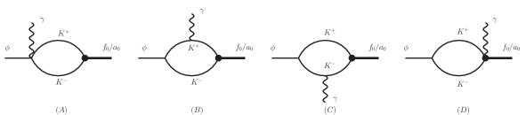
Figure 6: Diagrams contributing to the $\phi\to f_{0}/a_{0}\gamma$ Decay (without intermediate resonance contribution).

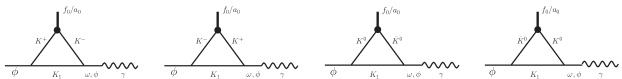
Figure 7: VMD diagrams contributing to the $\phi\to f_{0}/a_{0}\gamma$ Decay.

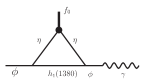
Figure 8: VMD diagrams contributing to the $\phi\to f_{0}\gamma$ Decay (contribution from the $\eta$ constituent of $f_{0}$).

Before explicit calculation, we will discuss the interaction Lagrangian to be used in the following. At first, the $\phi KK$ interaction Lagrangian can be effectively written as

$${\cal L}_{\phi KK} = ig_{\phi KK}\phi_{\mu}K^{{\dagger}}(x)\partial_{\mu}^{{}^{{}^{\leftrightarrow}}}K(x)$$ (108)

Using the data for the strong decay width $\Gamma(\phi\to K^{+}K^{-}=4.26{~{}\rm MeV}\times 49.2\%=2.096{~{}\rm MeV}$ Amsler:2008zz , one can fix the coupling constant $g_{\phi KK}$. In particular the strong decay width $\Gamma(\phi\to K^{+}K^{-})$ relates to $g_{\phi KK}$ via

$$\Gamma(\phi\to KK) = \frac{g_{\phi KK}^{2}}{6\pi m_{\phi}^{2}}P_{\phi K}^{3}$$ (109)

where $P_{\phi K}$ is the three-momentum of $K$ in the rest frame of $\phi$. Using the masses for the relevant mesons one can deduce $g_{\phi KK}=4.48$.

The interaction Lagrangian between photon and vector meson is given by Harada:2003jx

$${\cal L}_{V\gamma} = -4F_{\pi}^{2}eg_{\rho\pi\pi}A_{\mu}{\rm Tr}[QV_{\mu}]=-\frac{2F_{\pi}^{2}eg_{\rho\pi\pi}}{3}A_{\mu}\omega_{\mu}+\frac{2\sqrt{2}F_{\pi}^{2}eg_{\rho\pi\pi}}{3}A_{\mu}\phi_{\mu}$$ (110)

where $Q=(2/3,-1/3,-1/3)$ is the quark electric charge matrix and, the vector meson matrix is chosen as

$$V_{\mu} = \frac{1}{2}\left(\begin{array}[]{ccc}\rho^{0}+\omega&\sqrt{2}\rho^{+}&\sqrt{2}K^{\ast+}\\ \sqrt{2}\rho^{-}&-\rho^{0}+\omega&\sqrt{2}K^{\ast 0}\\ \sqrt{2}K^{\ast-}&\sqrt{2}\bar{K}^{\ast 0}&\sqrt{2}\phi\\ \end{array}\right)_{\mu}$$ (114)

and $g_{\rho\pi\pi}=5.98$ is the universal $\rho\pi\pi$ coupling constant.

To include the axial-vector mesons, according to PDG Amsler:2008zz , one should consider two nonets with quantum numbers $J^{PC}=1^{+-}$ and $1^{++}$. Explicitly, they can be written in $U(3)$ matrix forms as

$$A_{\mu} = \left(\begin{array}[]{ccc}a_{1}^{0}+f_{1}(1285)&\sqrt{2}a_{1}^{+}&\sqrt{2}K_{1A}^{+}\\ \sqrt{2}a_{1}^{-}&-a_{1}^{0}+f_{1}(1285)&\sqrt{2}K_{1A}^{0}\\ \sqrt{2}K_{1A}^{-}&\sqrt{2}\bar{K}_{1A}^{0}&f_{1}(1420)\\ \end{array}\right)_{\mu}$$ (118)

$$B_{\mu} = \left(\begin{array}[]{ccc}b_{1}^{0}+h_{1}(1170)&\sqrt{2}b_{1}^{+}&\sqrt{2}K_{1B}^{+}\\ \sqrt{2}b_{1}^{-}&-b_{1}^{0}+h_{1}(1170)&\sqrt{2}K_{1B}^{0}\\ \sqrt{2}K_{1B}^{-}&\sqrt{2}\bar{K}_{1B}^{0}&h_{1}(1380)\\ \end{array}\right)_{\mu}$$ (122)

where $A_{\mu}$ and $B_{\mu}$ are the axial-vector matrices with quantum numbers $J^{PC}=1^{++}$ and $1^{+-}$, respectively. The mixture of $K_{iA}$ and $K_{1B}$ with approximate $45^{\circ}$ mixing angle gives the physical states $K_{1}(1270)$ and $K_{1}(1400)$. Explicitly

$$K_{1}(1270) = \frac{1}{\sqrt{2}}(K_{1B}-iK_{1A})$$

$$K_{1}(1400) = \frac{1}{\sqrt{2}}(K_{1B}+iK_{1A})$$ (123)

Due to the $C$ parity, the interaction Lagrangian for the axial-vector-vector-pseudoscalar couplings have the following forms

$${\cal L}_{AVP} = ig_{{}_{AVP}}{\rm Tr}\Big{[}\;A_{\mu}[\;V_{\mu},P\;]\Big{]}$$

$${\cal L}_{BVP} = g_{{}_{BVP}}{\rm Tr}\Big{[}\;B_{\mu}\{\;V_{\mu},P\;\}\Big{]}$$ (124)

where $i$ in front of $g_{{}_{AVP}}$ was added to keep the Hermitian of the Lagrangian. Using the concrete matrix forms, one can write down the interaction vertices that we are interested in

$${\cal L}_{AVP} = \sqrt{2}g_{{}_{AVP}}\Big{[}K_{1;\mu}^{+}(1270)\rho_{\mu}^{0}K^{-}-K_{1;\mu}^{+}(1400)\rho_{\mu}^{0}K^{-}$$

$$\;\;\;\;\;\;\;\;\;\;\;\;\;\;\;+\sqrt{2}K_{1;\mu}^{+}(1270)\rho_{\mu}^{-}\bar{K}^{0}-\sqrt{2}K_{1;\mu}^{+}(1400)\rho_{\mu}^{-}\bar{K}^{0}\Big{]}$$

$$+\sqrt{2}g_{{}_{AVP}}\phi_{\mu}\Big{[}K_{1;\mu}^{+}(1400)K^{-}-K_{1;\mu}^{+}(1270)K^{-}+K_{1;\mu}^{0}(1400)\bar{K}^{0}-K_{1;\mu}^{0}(1270)\bar{K}^{0}\Big{]}$$

$$-\sqrt{2}g_{{}_{AVP}}\omega_{\mu}\Big{[}K_{1;\mu}^{+}(1400)K^{-}-K_{1;\mu}^{+}(1270)K^{-}+K_{1;\mu}^{0}(1400)\bar{K}^{0}-K_{1;\mu}^{0}(1270)\bar{K}^{0}\Big{]}+{\rm H.c.}$$

$${\cal L}_{BVP} = \sqrt{2}g_{{}_{BVP}}\Big{[}K_{1;\mu}^{+}(1400)\rho_{\mu}^{0}K^{-}+K_{1;\mu}^{+}(1270)\rho_{\mu}^{0}K^{-}$$ (125)

$$\;\;\;\;\;\;\;\;\;\;\;\;\;\;\;+\sqrt{2}K_{1;\mu}^{+}(1400)\rho_{\mu}^{-}\bar{K}^{0}+\sqrt{2}K_{1;\mu}^{+}(1270)\rho_{\mu}^{-}\bar{K}^{0}\Big{]}$$

$$+\sqrt{2}g_{{}_{BVP}}\phi_{\mu}\Big{[}K_{1;\mu}^{+}(1400)K^{-}+K_{1;\mu}^{+}(1270)K^{-}+K_{1;\mu}^{0}(1400)\bar{K}^{0}+K_{1;\mu}^{0}(1270)\bar{K}^{0}\Big{]}$$

$$+\sqrt{2}g_{{}_{BVP}}\omega_{\mu}\Big{[}K_{1;\mu}^{+}(1400)K^{-}+K_{1;\mu}^{+}(1270)K^{-}+K_{1;\mu}^{0}(1400)\bar{K}^{0}+K_{1;\mu}^{0}(1270)\bar{K}^{0}\Big{]}+{\rm H.c.}$$

$$-\frac{4g_{{}_{BVP}}}{\sqrt{3}}\phi_{\mu}h_{1;\mu}(1380)\eta+\frac{2g_{{}_{BVP}}}{\sqrt{3}}\omega_{\mu}(b_{1;\mu}^{0}+h_{1;\mu}(1170)\eta$$

The coupling constant $g_{{}_{K_{1}VP}}$ can be determined by the decays of $K_{1}\to\rho K$ via the expression

$$\Gamma(K_{1}\to VP) = \frac{g_{{}_{K_{1}VP}}^{2}}{24\pi m_{{}_{K_{1}}}^{2}}{\rm P}_{K_{1}V}\Big{[}3+\frac{1}{m_{{}_{V}}^{2}}{\rm P}_{K_{1}V}^{2}\Big{]}$$ (126)

where $g_{{}_{K_{1}VP}}$ is the relevant coupling constant and ${\rm P}_{K_{1}V}$ is the three momentum of $V-$meson in the rest frame of $K_{1}-$meson. Explicitly, $g_{{}_{K_{1}(1270)^{+}\rho^{0}K^{-}}}=\sqrt{2}(g_{{}_{AVP}}+g_{{}_{BVP}})$ and $g_{{}_{K_{1}(1400)^{+}\rho^{0}K^{-}}}=\sqrt{2}(g_{{}_{BVP}}-g_{{}_{AVP}})$. Using the central values of the branching ratio and total widths from PDG Amsler:2008zz $\Gamma(K_{1}(1270)\to\rho K)=37.8{~{}\rm MeV}$ and $\Gamma(K_{1}(1400)\to\rho K)=5.22{~{}\rm MeV}$ one can get

$$g_{{}_{K_{1}(1270)^{+}\rho^{0}K^{-}}} = 3.52~{}{\rm GeV};\;\;\;\;g_{{}_{K_{1}(1400)^{+}\rho^{0}K^{-}}}=0.54~{}{\rm GeV}$$ (127)

which lead to

$$g_{{}_{AVP}} = 1.05~{}{\rm GeV};\;\;\;\;g_{{}_{BVP}}=1.44~{}{\rm GeV}$$ (128)

We would like to mention that, in the following calculation, we will not include the diagrams arise from the $\phi-\omega$ mixing. This is because, the interaction Lagrangian describing the $\phi-\omega$ mixing is Urech:1995ry

$${\cal L}_{\phi\omega} = \Theta\phi_{\mu}\omega_{\mu}$$ (129)

where the coupling constant $\Theta$ is determined by the relation Bramon:1997va

$$\tilde{\epsilon} = \frac{\Theta}{m_{\phi}^{2}-m_{\omega}^{2}}=0.059\pm 0.004$$ (130)

all the diagrams with $\phi-\omega$ are suppressed by factor $\tilde{\epsilon}$ compared with the diagrams without $\phi-\omega$ mixing.

With the above discussions, we can calculate the decay width now. Generally, due to the gauge invariance, one can write the total matrix element as

$$iM(\phi(p)\to S(p^{\prime})\gamma(q)) = i\epsilon_{\mu}(p)\epsilon_{\nu}^{\ast}(q)(g_{\mu\nu}p\cdot q-q_{\mu}p_{\nu})\;e\;G_{\phi S\gamma}$$ (131)

and the effective coupling constant $G_{\phi S\gamma}$ consists of two parts

$$G_{\phi S\gamma} = G_{\phi S\gamma}^{c}+G_{\phi S\gamma}^{r}$$ (132)

where $G_{\phi S\gamma}^{c}$ is from Fig. 6, and $G_{\phi S\gamma}^{r}$ is from Figs. 7 and 8. The decay width can be expressed as

$$\Gamma(\phi\to S\gamma) = \frac{\alpha_{\rm em}}{3}|G_{\phi S\gamma}|^{2}P_{\gamma}^{\ast~{}3}$$ (133)

where $P_{\gamma}^{\ast}=(m_{\phi}^{2}-m_{S}^{2})/(2m_{\phi})$ is the three-momentum of the decay products.

With these discussions and selecting $\Lambda=1.5~{}$GeV which means the resonances with masses below $1.5~{}$GeV were included, one can do the numerical calculation. Using the effective coupling constants, we get the decay widths from the contact diagrams and the resonances as

$$\Gamma(\phi\to f_{0}\gamma)^{c} = 3.080\times 10^{-4}{~{}\rm MeV}\;\;;\;\;\Gamma(\phi\to a_{0}\gamma)^{c}=2.329\times 10^{-4}{~{}\rm MeV}$$

$$\Gamma(\phi\to f_{0}\gamma)^{r} = 6.670\times 10^{-13}{~{}\rm MeV}\;\;;\;\;\Gamma(\phi\to a_{0}\gamma)^{r}=3.353\times 10^{-13}{~{}\rm MeV}$$ (134)

From these results we see, compared with the contact diagrams, the contribution from the axial-vector resonances is negligible. In summary we have the total decay widths and the branching ratios (using the total width $\Gamma_{\phi}=4.46$ MeV Amsler:2008zz ) as

$$\Gamma(\phi\to f_{0}\gamma) = 3.081\times 10^{-4}{~{}\rm MeV};\;\;\;\;\;\;\Gamma(\phi\to a_{0}\gamma)=2.329\times 10^{-4}{~{}\rm MeV}$$

$${\rm Br}(\phi\to f_{0}\gamma) = 6.907\times 10^{-5};\;\;\;\;\;\;\;\;\;\;\;\;\;\;{\rm Br}(\phi\to a_{0}\gamma)=5.223\times 10^{-5}$$ (135)

and the ratio

$$R = \frac{\Gamma(\phi\to f_{0}\gamma)}{\Gamma(\phi\to a_{0}\gamma)}=1.32$$ (136)

Table 3: The branch ratio of the $\phi\to f_{0}/a_{0}\gamma$ decays.

Decay modes	Present results	SND	CLOE	CMD-2
${\rm Br}(\phi\to f_{0}\gamma)$	$6.91\times 10^{-5}$	$3.5\times 10^{-4}$ Achasov:2000ym	$(4.47\pm 0.21)\times 10^{-4}$Aloisio:2002bt	$2.90\times 10^{-4}$Akhmetshin:1999di
${\rm Br}(\phi\to a_{0}\gamma)$	$5.22\times 10^{-5}$	$8.8\times 10^{-5}$ Achasov:2000ku	$(7.4\pm 0.7)\times 10^{-5}$ Aloisio:2002bsa	$9.0\times 10^{-5}$ Akhmetshin:1999di
$\frac{{\rm Br}(\phi\to f_{0}\gamma)}{{\rm Br}(\phi\to a_{0}\gamma)}$	$1.32$	$3.98$	$6.04$	$3.22$

In Table. 3, we compare our results with that from the data. From this table one can see that, for the decay $\phi\to a_{0}\gamma$, the present branching ratio is consistent with the observed data while, that for the decay $\phi\to f_{0}\gamma$ is much smaller than data. This fact makes $R={\rm Br}(\phi\to f_{0}\gamma)/{\rm Br}(\phi\to a_{0}\gamma)=1.32$ disagree with the data. Actually, as mentioned in Ref. Close:2002zu , this is one of the main problems in the hadronic interpretation of the light scalar mesons. Another observation is that, the final state interaction gives a negligible contribution to these decays which agrees with the conclusion given in Ref. Palomar:2003rb .

V Discussions and Conclusions

In this paper, in the framework of effective Lagrangian approach, we studied the properties of the light scalar mesons with masses below 1.0 GeV in the hadronic molecular interpretation.

To determine the coupling constant $g_{{}_{S}}$ between the scalar molecule and its constituents we applied the compositeness condition which has been used in our previous works. We found the numerical results of $g_{{}_{S}}$ are consistent with that given in the literature. With the yielded coupling constant $g_{{}_{S}}$ we calculated the leptonic decay constants and leptonic decay widths of scalar mesons. Our numerical results show that the leptonic decays of scalar mesons are not observable in the near future experiments.

The calculations of the strong decays conclude that the decay widths for $f_{0}\to\pi\pi$ and $a_{0}\to\eta\pi$ is consistent with the observed data while width for $K_{0}^{\ast}\to K\pi$ decay is much smaller than the data, even the ambiguity from the mass is considered. This observation shows that the hadronic molecular interpretation of $K_{0}^{\ast}$ is disputable and, concerning the $f_{0}\to\pi\pi$ and $a_{0}\to\eta\pi$ decays are consistent with the data, the classification of the scalar mesons with masses below $1.0~{}$GeV to form a nonet is disputable.

To study the productions of $f_{0}$ and $a_{0}$ in the radiative decays of $\phi$ meson, we included the contributions from the final state interaction, i.e., the contributions from the intermediate axial-vector mesons. The explicit calculation shows that the dominant contribution is from the contact diagrams of kaon loops and axial-vector mesons play a negligible role in these processes. The branching ratio for $\phi\to a_{0}\gamma$ is consistent with the data while that for $\phi\to f_{0}\gamma$ is much smaller than the data. This is another problem of the hadronic molecular model.

We would like to say that, if the isosinglet pseudoscalar constituent $\eta$ is substituted by $\eta^{\prime}$, the width for decay $K_{0}^{\ast}\to K\pi$ is not improved but suppressed. In fact, when $\eta$ meson is substituted by $\eta^{\prime}$ meson, the coupling constant $g_{{}_{K_{0}^{\ast\pm}}}$ is improved to $g_{{}_{K_{0}^{\ast\pm}}}=20.54~{}{\rm GeV}$, but coupling constant $g_{K^{\ast}K\eta^{\prime}}$ is suppressed to $g_{K^{\ast}K\eta^{\prime}}=1.095$ when the mixing angle $\theta_{P}=-9.95^{\circ}$ Venugopal:1998fq and $f_{8}=1.26f_{\pi}$ Feldmann:1998vh are applied. So that, compared to the $\eta$ meson case, the partial width $\Gamma(K_{0}^{\ast+}\to K\pi)$ from the final state interaction is suppressed by a factor $(20.54\times 1.095)^{2}/(12.99\times 6.14)^{2}\simeq 0.078$. For the contribution from the contact diagram, explicit calculation shows that the partial width due to this diagram is about 34% of that of the $\eta$ meson case. So that the partial width from the sum of these two diagrams is about one third of that of the $\eta$ meson case.

One may notice that another possibility to improve the numerical value of the width for decay $K_{0}^{\ast}\to K\pi$ is to enlarge the parameter $\Lambda$ in the form factor $\mathcal{F}(q^{2})$. In fact, we check that to make the numerical value of the width for decay $K_{0}^{\ast}\to K\pi$ agrees with the data, $\Lambda\simeq 1.5~{}$GeV. But in this case, $\Gamma(a_{0}^{+}\to\eta\pi^{+})=749~{}$MeV and $\Gamma(a_{0}^{0}\to\eta\pi^{0})=665~{}$MeV. Both of them are much larger than the data.

At last, we would like to mention that, we have estimated the decay of $K_{0}^{\ast}(1430)\to K\pi$ rudely. In this case, the singlet must be $\eta^{\prime}$. Our result for the partial width is $\sim 124.0~{}$MeV which is about a half of the data and the improvement is mainly from the phase space. In this sense, it seems that $\sigma(600),f_{0}(980),a_{(}980)$ and $K_{0}^{\ast}(1430)$ can be classified into a same nonet. However, this deserves further systematically study.

In conclusion, our explicit result shows that, in the hadronic molecular model, it is difficult to arrange the scalar mesons with masses below 1.0 GeV in the same nonet.

Appendix A Integral formulas

In this appendix, we will derive some integral formulae of the one-loop integrals for $a_{0}\to\eta\pi$ decay. To derive the relations we have used $p=p_{1}+p_{2}$ and $p^{2}=m_{S}^{2},p_{i}^{2}=m_{i}^{2}$.

A.1 Integral formulae for the contact diagram

In this subsection, we will reduce the momentum integral for the contact diagram to the standard loop integral function. For $I_{D}^{(A)}$, one has

$$I_{D}^{(A)}(m_{S};M_{c_{1}},M_{c_{2}};m_{1},m_{2}) = g_{P_{1}P_{2}P_{3}P_{4}}^{D}\int\frac{d^{4}k}{(2\pi)^{4}}\mathcal{F}(k^{2})\frac{i}{k^{2}-M_{c_{1}}^{2}}\frac{i}{(k+p)^{2}-M_{c_{2}}^{2}}$$ (137)

$$\;\;\;\;\;\;\;\;\;\;\;\;\times\Big{[}[(k+p)+p_{1}]\cdot(k-p_{2})+(p_{1}-k)\cdot[-p_{1}-(k+p)]\Big{]}$$

$$= -ig_{P_{1}P_{2}P_{3}P_{4}}^{D}\Big{[}-(3m_{S}^{2}-m_{1}^{2}-m_{2}^{2}-\Lambda^{2}-M_{c_{2}}^{2})$$

$$\;\;\;\;\;\;\;\;\;\;\;\;\;\;\;\;\;\;\;\;\;\times I_{0}(m_{S};M_{c_{1}},M_{c_{2}};\Lambda)$$

$$\;\;\;\;\;\;\;\;\;\;\;\;\;\;\;\;\;\;\;\;\;+I_{2}^{(a)}(m_{S};M_{c_{1}},M_{c_{2}};\Lambda)+I_{2}^{(b)}(M_{c_{1}};\Lambda)\Big{]}$$

where the relevant functions are defined as

$$I_{2}^{(a)}(m_{S};M_{c_{1}},M_{c_{2}};\Lambda) = \frac{1}{i}\int\frac{d^{4}k}{(2\pi)^{4}}{\cal F}(k^{2})\frac{1}{k^{2}-M_{c_{1}}^{2}}\frac{k^{2}-\Lambda^{2}}{(k+p)^{2}-M_{c_{2}}^{2}}$$

$$= (M_{c_{1}}^{2}-\Lambda^{2})\frac{1}{16\pi^{2}}[B_{0}(m_{S}^{2},M_{c_{1}}^{2},M_{c_{2}}^{2})-B_{0}(m_{S}^{2},\Lambda^{2},M_{c_{2}}^{2})]$$

$$I_{2}^{(b)}(M_{c_{1}};\Lambda) = \frac{1}{i}\int\frac{d^{4}k}{(2\pi)^{4}}{\cal F}(k^{2})\frac{1}{k^{2}-M_{c_{1}}^{2}}$$

$$= \frac{1}{16\pi^{2}}[A_{0}(M_{c_{1}}^{2})-A_{0}(\Lambda^{2})-(M_{c_{1}}^{2}-\Lambda^{2})\frac{d}{d\Lambda^{2}}A_{0}(\Lambda^{2})]$$

$$I_{0}(m_{S};M_{c_{1}},M_{c_{2}};\Lambda) = \frac{1}{i}\int\frac{d^{4}k}{(2\pi)^{4}}{\cal F}(k^{2})\frac{1}{k^{2}-M_{c_{1}}^{2}}\frac{1}{(k+p)^{2}-M_{c_{2}}^{2}}$$ (138)

$$= \frac{1}{16\pi^{2}}[B_{0}(m_{S}^{2},M_{c_{1}}^{2},M_{c_{2}}^{2})-B_{0}(m_{S}^{2},\Lambda^{2},M_{c_{2}}^{2})$$

$$\;\;\;\;\;\;\;\;\;\;-(M_{c_{1}}^{2}-\Lambda^{2})\frac{d}{d\Lambda^{2}}B_{0}(m_{S}^{2},\Lambda^{2},M_{c_{2}}^{2})]$$

And for $I_{ND}^{(A)}$ we have

$$I_{ND}^{(A)}(m_{S};M_{1},M_{2}) = g_{P_{1}P_{2}P_{3}P_{4}}^{ND}~{}\int\frac{d^{4}k}{(2\pi)^{4}}\mathcal{F}(k^{2})\frac{i}{k^{2}-m_{c_{1}}^{2}}\frac{i}{(k+p)^{2}-m_{c_{2}}^{2}}$$ (139)

$$= -ig_{P_{1}P_{2}P_{3}P_{4}}^{ND}~{}I_{0}(m_{S};M_{c_{1}},M_{c_{2}};\Lambda)$$

A.2 Integral formulae for the final state interaction diagram

In this subsection, we will reduce the momentum integral for the final state interaction diagram to the standard loop integral function. After some algebra, one has

$$I^{(B)}(m_{S};M_{c_{1}},M_{c_{2}};m_{V};m_{1},m_{2}) = \int\frac{d^{4}k}{(2\pi)^{4}}{\cal F}(k^{2})\frac{i}{(k-p_{1})^{2}-m_{c_{1}}^{2}}\frac{i}{(k+p_{2})^{2}-m_{c_{2}}^{2}}\frac{-i}{k^{2}-m_{V}^{2}}$$ (140)

$$\times(2p_{1}-k)_{\mu}[g_{\mu\nu}-\frac{k_{\mu}k_{\nu}}{m_{K^{\ast}}^{2}}](k+2p_{2})_{\nu}$$

$$= I_{0}^{(a)}(m_{S};M_{c_{1}},M_{c_{2}};m_{V};m_{1},m_{2};\Lambda)+\frac{1}{m_{V}^{2}}I_{2}^{(a)}(m_{V};\Lambda)$$

$$-[1-\frac{1}{m_{V}^{2}}(M_{c_{2}}^{2}-m_{2}^{2})]I_{0}^{(b)}(M_{c_{2}};m_{V};m_{2};\Lambda)$$

$$-[1-\frac{1}{m_{V}^{2}}(M_{c_{1}}^{2}-m_{1}^{2})]I_{0}^{(c)}(M_{c_{1}},m_{V};m_{1};\Lambda)$$

$$-\Big{[}M_{c_{1}}^{2}+M_{c_{2}}^{2}-m_{V}^{2}-2m_{S}^{2}+m_{1}^{2}+m_{2}^{2}$$

$$\;\;\;\;\;-\frac{1}{m_{V}^{2}}(M_{c_{1}}^{2}-m_{1}^{2})(M_{c_{2}}^{2}-m_{2}^{2})\Big{]}$$

$$\times I_{-2}(m_{S};M_{c_{1}},M_{c_{2}};m_{V};m_{1},m_{2};\Lambda)$$

where

$$I_{0}^{(a)}(m_{S};M_{c_{1}},M_{c_{2}};m_{V};m_{1},m_{2};\Lambda) = \frac{1}{i}\int\frac{d^{4}k}{(2\pi)^{4}}{\cal F}(k^{2})$$

$$\times\frac{1}{(k-p_{1})^{2}-M_{c_{1}}^{2}}\frac{1}{(k+p_{2})^{2}-M_{c_{2}}^{2}}\frac{k^{2}-\Lambda^{2}}{k^{2}-m_{V}^{2}}$$

$$= (m_{V}^{2}-\Lambda^{2})\frac{1}{16\pi^{2}}[C_{0}(m_{1}^{2},m_{2}^{2},m_{S}^{2},M_{c_{1}}^{2},m_{V}^{2},m_{c_{2}}^{2})$$

$$\;\;\;\;\;\;\;\;\;\;\;\;\;\;\;\;\;\;\;\;\;\;\;\;\;\;\;\;-C_{0}(m_{1}^{2},m_{2}^{2},m_{S}^{2},M_{c_{1}}^{2},\Lambda^{2},m_{c_{2}}^{2})]$$

$$I_{0}^{(b)}(M_{c_{2}};m_{V};m_{2};\Lambda) = \frac{1}{i}\int\frac{d^{4}k}{(2\pi)^{4}}{\cal F}(k^{2})\frac{1}{(k+p_{2})^{2}-M_{c_{2}}^{2}}\frac{1}{k^{2}-m_{V}^{2}}$$

$$= \frac{1}{16\pi^{2}}[B_{0}(m_{2}^{2},m_{V}^{2},m_{c_{2}}^{2})-B_{0}(m_{2}^{2},\Lambda^{2},m_{c_{2}}^{2})$$

$$\;\;\;\;\;\;\;\;\;\;-(m_{V}^{2}-\Lambda^{2})\frac{d}{d\Lambda^{2}}B_{0}(m_{2}^{2},\Lambda^{2},m_{c_{2}}^{2})]$$

$$I_{0}^{(c)}(M_{c_{1}};m_{V};m_{1};\Lambda) = \frac{1}{i}\int\frac{d^{4}k}{(2\pi)^{4}}{\cal F}(k^{2},\Lambda^{2})\frac{1}{(k+p_{1})^{2}-M_{c_{1}}^{2}}\frac{1}{k^{2}-m_{V}^{2}}$$

$$= \frac{1}{16\pi^{2}}[B_{0}(m_{1}^{2},m_{V}^{2},m_{c_{1}}^{2})-B_{0}(m_{1}^{2},\Lambda^{2},m_{c_{1}}^{2})$$

$$\;\;\;\;\;\;\;\;\;\;-(m_{V}^{2}-\Lambda^{2})\frac{d}{d\Lambda^{2}}B_{0}(m_{1}^{2},\Lambda^{2},m_{c_{1}}^{2})]$$

$$I_{2}^{(a)}(m_{V};\Lambda) = \frac{1}{i}\int\frac{d^{4}k}{(2\pi)^{4}}{\cal F}(k^{2})\frac{1}{k^{2}-m_{V}^{2}}$$

$$= \frac{1}{16\pi^{2}}[A_{0}(m_{V}^{2})-A_{0}(\Lambda^{2})-(m_{V}^{2}-\Lambda^{2})\frac{d}{d\Lambda^{2}}A_{0}(\Lambda^{2})]$$

$$I_{-2}(m_{S};M_{c_{1}},M_{c_{2}};m_{V};m_{1},m_{2};\Lambda) = \frac{1}{i}\int\frac{d^{4}k}{(2\pi)^{4}}{\cal F}(k^{2})$$ (141)

$$\times\frac{1}{(k-p_{1})^{2}-M_{c_{1}}^{2}}\frac{1}{(k+p_{2})^{2}-M_{c_{2}}^{2}}\frac{1}{k^{2}-m_{V}^{2}}$$

$$= \frac{1}{16\pi^{2}}[C_{0}(m_{1}^{2},m_{2}^{2},m_{S}^{2},M_{c_{1}}^{2},m_{V}^{2},m_{c_{2}}^{2})$$

$$\;\;\;\;\;\;\;\;\;\;-C_{0}(m_{1}^{2},m_{2}^{2},m_{S}^{2},M_{c_{1}}^{2},\Lambda^{2},m_{c_{2}}^{2})$$

$$\;\;\;\;\;\;\;\;\;\;-(m_{V}^{2}-\Lambda^{2})\frac{d}{d\Lambda^{2}}C_{0}(m_{1}^{2},m_{2}^{2},m_{S}^{2},M_{c_{1}}^{2},\Lambda^{2},m_{c_{2}}^{2})]$$

References

• (1) C. Amsler et al. [Particle Data Group], Phys. Lett.  B 667, 1 (2008).
• (2) S. Godfrey and J. Napolitano, Rev. Mod. Phys.  71, 1411 (1999) [arXiv:hep-ph/9811410].
• (3) F. E. Close and N. A. Tornqvist, J. Phys. G 28, R249 (2002) [arXiv:hep-ph/0204205].
• (4) R. L. Jaffe, Phys. Rev.  D 15, 267 (1977).
• (5) R. L. Jaffe, Phys. Rev.  D 15, 281 (1977).
• (6) M. G. Alford and R. L. Jaffe, Nucl. Phys.  B 578, 367 (2000) [arXiv:hep-lat/0001023].
• (7) L. Maiani, F. Piccinini, A. D. Polosa and V. Riquer, Phys. Rev. Lett.  93, 212002 (2004) [arXiv:hep-ph/0407017].
• (8) J. A. Oller, E. Oset and J. R. Pelaez, Phys. Rev.  D 59, 074001 (1999) [Erratum-ibid.  D 60, 099906 (1999 ERRAT,D75,099903.2007)] [arXiv:hep-ph/9804209].
• (9) M. Ishida, Prog. Theor. Phys.  101, 661 (1999) [arXiv:hep-ph/9902260].
• (10) M. D. Scadron, G. Rupp, F. Kleefeld and E. van Beveren, Phys. Rev.  D 69, 014010 (2004) [Erratum-ibid.  D 69, 059901 (2004)] [arXiv:hep-ph/0309109].
• (11) N. A. Tornqvist, Eur. Phys. J.  C 11, 359 (1999) [arXiv:hep-ph/9905282].
• (12) N. A. Tornqvist, Z. Phys.  C 68, 647 (1995) [arXiv:hep-ph/9504372].
• (13) J. D. Weinstein and N. Isgur, Phys. Rev.  D 41, 2236 (1990).
• (14) J. R. Pelaez, Mod. Phys. Lett.  A 19, 2879 (2004) [arXiv:hep-ph/0411107].
• (15) J. R. Pelaez, Phys. Rev. Lett.  92, 102001 (2004) [arXiv:hep-ph/0309292].
• (16) J. R. Pelaez and G. Rios, Phys. Rev. Lett.  97, 242002 (2006) [arXiv:hep-ph/0610397].
• (17) F. Giacosa, T. Gutsche and V. E. Lyubovitskij, Phys. Rev.  D 77, 034007 (2008) [arXiv:0710.3403 [hep-ph]].
• (18) T. Branz, T. Gutsche and V. E. Lyubovitskij, Eur. Phys. J.  A 37, 303 (2008) [arXiv:0712.0354 [hep-ph]].
• (19) T. Branz, T. Gutsche and V. E. Lyubovitskij, Phys. Rev.  D 78, 114004 (2008) [arXiv:0808.0705 [hep-ph]].
• (20) T. Branz, T. Gutsche and V. E. Lyubovitskij, AIP Conf. Proc.  1030, 118 (2008) [arXiv:0805.1647 [hep-ph]].
• (21) T. Branz, T. Gutsche and V. E. Lyubovitskij, arXiv:0812.0942 [hep-ph].
• (22) A. Faessler, T. Gutsche, M. A. Ivanov, V. E. Lyubovitskij and P. Wang, Phys. Rev.  D 68, 014011 (2003) [arXiv:hep-ph/0304031].
• (23) E. van Beveren and G. Rupp, Eur. Phys. J.  C 22, 493 (2001) [arXiv:hep-ex/0106077].
• (24) L. S. Celenza, S. f. Gao, B. Huang, H. Wang and C. M. Shakin, Phys. Rev.  C 61, 035201 (2000).
• (25) Y. B. Dai and Y. L. Wu, Eur. Phys. J.  C 39, S1 (2005) [arXiv:hep-ph/0304075].
• (26) Bhavyashri, K. B. Vijaya Kumar, Y. L. Ma and A. Prakash, arXiv:0811.4308 [hep-ph].
• (27) H. Y. Cheng, arXiv:0901.0741 [hep-ph].
• (28) A. Faessler, T. Gutsche, V. E. Lyubovitskij and Y. L. Ma, Phys. Rev.  D 76, 014005 (2007) [arXiv:0705.0254 [hep-ph]].
• (29) A. Faessler, T. Gutsche, V. E. Lyubovitskij and Y. L. Ma, Phys. Rev.  D 76, 114008 (2007) [arXiv:0709.3946 [hep-ph]].
• (30) Y. b. Dong, A. Faessler, T. Gutsche and V. E. Lyubovitskij, Phys. Rev.  D 77, 094013 (2008) [arXiv:0802.3610 [hep-ph]].
• (31) A. Faessler, T. Gutsche, V. E. Lyubovitskij and Y. L. Ma, arXiv:0801.2232 [hep-ph].
• (32) Y. L. Ma, J. Phys. G 36, 055004 (2009) [arXiv:0808.3764 [hep-ph]].
• (33) M. Napsuciale and S. Rodriguez, Phys. Rev.  D 70, 094043 (2004) [arXiv:hep-ph/0407037].
• (34) J. J. Wu, Q. Zhao and B. S. Zou, Phys. Rev.  D 75, 114012 (2007) [arXiv:0704.3652 [hep-ph]].
• (35) J. J. Wu and B. S. Zou, Phys. Rev.  D 78, 074017 (2008) [arXiv:0808.2683 [hep-ph]].
• (36) P. Herrera-Siklody, J. I. Latorre, P. Pascual and J. Taron, Nucl. Phys.  B 497, 345 (1997) [arXiv:hep-ph/9610549].
• (37) M. Harada and J. Schechter, Phys. Rev.  D 54, 3394 (1996) [arXiv:hep-ph/9506473].
• (38) J. Gasser and H. Leutwyler, Annals Phys.  158, 142 (1984).
• (39) J. Gasser and H. Leutwyler, Nucl. Phys.  B 250, 465 (1985).
• (40) R. Machleidt, K. Holinde and C. Elster, Phys. Rept.  149 (1987) 1.
• (41) T. Hahn and M. Perez-Victoria, Comput. Phys. Commun.  118, 153 (1999) [arXiv:hep-ph/9807565].
• (42) F. Giacosa, Phys. Rev.  D 74, 014028 (2006) [arXiv:hep-ph/0605191].
• (43) J. E. Palomar, L. Roca, E. Oset and M. J. Vicente Vacas, Nucl. Phys.  A 729, 743 (2003) [arXiv:hep-ph/0306249].
• (44) M. Harada and K. Yamawaki, Phys. Rept.  381 (2003) 1 [arXiv:hep-ph/0302103].
• (45) R. Urech, Phys. Lett.  B 355 (1995) 308 [arXiv:hep-ph/9504238].
• (46) A. Bramon, R. Escribano and M. D. Scadron, Eur. Phys. J.  C 7, 271 (1999) [arXiv:hep-ph/9711229].
• (47) M. N. Achasov et al., Phys. Lett.  B 485, 349 (2000) [arXiv:hep-ex/0005017].
• (48) M. N. Achasov et al., Phys. Lett.  B 479, 53 (2000) [arXiv:hep-ex/0003031].
• (49) A. Aloisio et al. [KLOE Collaboration], Phys. Lett.  B 537, 21 (2002) [arXiv:hep-ex/0204013].
• (50) A. Aloisio et al. [KLOE Collaboration], Phys. Lett.  B 536, 209 (2002) [arXiv:hep-ex/0204012].
• (51) R. R. Akhmetshin et al. [CMD-2 Collaboration], Phys. Lett.  B 462, 380 (1999) [arXiv:hep-ex/9907006].
• (52) E. P. Venugopal and B. R. Holstein, Phys. Rev.  D 57, 4397 (1998) [arXiv:hep-ph/9710382].
• (53) T. Feldmann, P. Kroll and B. Stech, Phys. Rev.  D 58, 114006 (1998) [arXiv:hep-ph/9802409].