Abstract

Based on the Lue-Starkman conjecture on the dynamical screening of the brane cosmological constant in the DGP scenario, we extend this proposal to a general DGP-inspired $F(R,\phi)$ Model. We show that modification of the induced gravity and its coupling to a quintessence field localized on the brane, affects the screening of the brane cosmological constant and also phantom-like behavior on the brane. We extend our study to possible modification of the induced gravity on the brane and for clarification some specific examples are presented. As a result, phantom-like behavior can be realized in this setup without violating the null energy condition at least in some subspaces of the model parameter space. The key result of our study is the fact that a DGP-inspired $F(R,\phi)$ scenario has the best fit with LCDM and recent observations than other alternative theories.
PACS: 04.50.-h, 98.80.-k
Key Words: Dark Energy, Scalar-Tensor Theories, Braneworld Cosmology

1 Introduction

Recent evidences from supernova searches data [1,2], cosmic microwave background (CMB) results [3-5] and also Wilkinson Microwave Anisotropy Probe (WMAP) data [6,7], show an positively accelerating phase of the cosmic expansion today and this feature shows that the simple picture of the universe consisting of the pressureless fluid is not enough to describe the cosmological dynamics. In this regard, the universe may contain some sort of the additional negative-pressure dark energy. Analysis of the WMAP data [8-10] shows that there is no indication for any significant deviations from Gaussianity and adiabaticity of the CMB power spectrum and therefore suggests that the universe is spatially flat to within the limits of observational accuracy. Further, the combined analysis of the WMAP data with the supernova Legacy survey (SNLS) [8], constrains the equation of state $w_{de}$, corresponding to almost ${74\%}$ contribution of dark energy in the currently accelerating universe, to be very close to that of the cosmological constant value. In this respect, a LCDM ( Cosmological constant plus Cold Dark Matter) model has maximum agreement with the recent data. Moreover, observations appear to favor a dark energy equation of state, $w_{de}<-1$ [11]. Therefore, a viable cosmological model should admit a dynamical equation of state that might have crossed the value $w_{de}=-1$ in the recent epoch of cosmological evolution [12]. In fact, to explain positively accelerated expansion of the universe, there are two alternative approaches: incorporating an additional cosmological component ( dark energy) in matter sector of the general theory of relativity ( $G_{\mu\nu}=8\pi G(T^{(M)}_{\mu\nu}+T^{(Dark)}_{\mu\nu})$  where $T^{(M)}_{\mu\nu}$ and $T^{(Dark)}_{\mu\nu}$ are energy-momentum tensor of ordinary matter and dark energy respectively), or modifying geometric sector of the theory (dark geometry)($G_{\mu\nu}+G^{Dark}_{\mu\nu}=8\pi GT^{(M)}_{\mu\nu}$) at the cosmological scales. Multi-component dark energy with at least one non-canonical phantom field is a possible candidate of the first alternative. This viewpoint has been studied extensively in the literature ( see [13,14] and references therein ). Another alternative to explain current accelerated expansion of the universe is extension of the general relativity to more general theories on cosmological scales. In this view point, modified Einstein-Hilbert action via $f(R)$-gravity ( see [15] and references therein) or braneworld gravity [16-18] are studied extensively. In this framework the geometric part of the Einstein’s field equations are modified. For instance, DGP ( Dvali-Gabadadze-Porrati) braneworld scenario as an IR modification of the general relativity explains accelerated expansion of the universe in its self-accelerating branch via leakage of gravity to extra dimension. In this model, equation of state parameter of dark energy never crosses the $\omega(z)=-1$ line, and universe eventually turns out to be de Sitter phase. Nevertheless, in this setup if we use a single scalar field (ordinary or phantom) on the brane, we can show that equation of state parameter of dark energy can cross phantom divide line [19]. One important consequence in the quintessence model of dark energy is the fact that a single minimally coupled scalar field has not the capability to explain crossing of the phantom divide line, $\omega_{\phi}=-1$ [20]. However, a single but non-minimally coupled scalar field is enough to cross the phantom divide line by its equation of state parameter [13,14]. Lorentz invariance violating vector fields in an interactive basis are other possibility to realize cosmological line crossing [21]. Lue and Starkman [22] based on the analysis firstly reported by Sahni and Shtanov [23] have shown that one can realize the phantom-like effect ( increasing of the effective dark energy density with cosmic time) in the normal branch of the DGP cosmological solution without introducing any phantom field. This type of the analysis then has been extended by several authors [24]. The normal branch of the model which cannot explain the self-acceleration, has the key property that brane is extrinsically curved so that shortcuts through the bulk allow gravity to screen the effects of the brane energy-momentum contents at Hubble parameters of the order of the inverse of crossover distance [22]. Since in this case $H(t)$ is a decreasing function of the cosmic time, the effective dark energy component is increasing with time and therefore we observe a phantom-like behavior without introducing any phantom matter. It is important to note that crossing of the phantom divide line in this viewpoint is impossible without introduction of a quintessence field on the brane [24]. This idea has been studied further to incorporate curvature effects [25]. The importance of this type of reasoning lies in the fact that we don’t need to introduce phantom fields that violate the null energy condition and suffer from several theoretical problems.

Here we are going to study phantom-like effect in the normal branch of a general DGP inspired $F(R,\phi)$ scenario. The DGP inspired $F(R,\phi)$ scenarios have been studied in Refs. [26,27]. Our motivation to study phantom-like behavior of this extension of the DGP scenario is the fact that to have crossing of the phantom divide line on the DGP brane we have to incorporate a quintessence field on the brane [24]. On the other hand, it is reasonable to assume that induced gravity on the brane can be modified. In fact, as has been argued in Refs [28], generalized version of DGP scenario ( such as modified induced gravity), can be ghost free and can give rise to transient acceleration ( see also [23] and [29]). Here we are focus on the normal branch of the scenario which is ghost-free. We show that for the case with $F(R,\phi)=\frac{1}{2}(1-\xi\phi^{2})R$, the effective dark energy density reduces by increasing the values of the non-minimal coupling, $\xi$. We extend our study to the general $f(R)$-gravity to explore the role played by the modification of the induced gravity on the screening of the brane cosmological constant and the phantom-like effect. We show that phantom-like behavior can be realized in this setup without violating the null energy condition at least in some subspaces of the model parameter space. The key result of our study is the fact that a DGP-inspired $F(R,\phi)$ scenario has the best fit with LCDM and recent observations.

2 Non-minimal DGP Cosmology

2.1 The Setup

The action of the DGP scenario in the presence of a non-minimally coupled scalar field on the brane can be written as follows [27]

$$S=\int d^{5}x\frac{m^{3}_{4}}{2}\sqrt{-g}{\cal R}+\Bigg{[}\int d^{4}x\sqrt{-q}\bigg{(}\frac{m_{3}^{2}}{2}\alpha(\phi)R[q]-\frac{1}{2}q^{\mu\nu}\nabla_{\mu}\phi\nabla_{\nu}\phi-V(\phi)+m^{3}_{4}\overline{K}+{\cal{L}}_{m}\bigg{)}\Bigg{]}_{y=0},$$ (1)

where we have included a general non-minimal coupling $\alpha(\phi)$  in the brane part of the action( for an interesting discussion on the possible schemes to incorporate NMC in the formulation of the scalar-tensor gravity see [30,26], and also [31] for a braneworld viewpoint).  $m_{3}^{2}=(8\pi G)^{-1}$ and $y$ is the coordinate of the fifth dimension and we assume that brane is located at $y=0$.  $g_{AB}$ is five dimensional bulk metric with Ricci scalar ${\cal{R}}$, while $q_{\mu\nu}$ is induced metric on the brane with induced Ricci scalar $R$.  $\overline{K}$ is trace of the mean extrinsic curvature of the brane defined as

$$\overline{K}_{\mu\nu}=\frac{1}{2}\,\,\lim_{\epsilon\rightarrow 0}\bigg{(}\Big{[}K_{\mu\nu}\Big{]}_{y=-\epsilon}+\Big{[}K_{\mu\nu}\Big{]}_{y=+\epsilon}\bigg{)},$$ (2)

and corresponding term in the action is York-Gibbons-Hawking term [33] (see also [34]). The ordinary matter part of the action is shown by the Lagrangian ${\cal{L}}_{m}\equiv{\cal{L}}_{m}(q_{\mu\nu},\psi)+\frac{\Lambda}{8\pi G}$ where $\psi$ is matter field and corresponding energy-momentum tensor is

$$T_{\mu\nu}=-2\frac{\delta{\cal{L}}_{m}}{\delta q^{\mu\nu}}+q_{\mu\nu}{\cal{L}}_{m},$$ (3)

and  $\Lambda$  is the brane cosmological constant. Note that we assume that in addition to brane cosmological constant, there is some quintessence scalar field localized on the brane to have a more general framework and in order to realize phantom divide line crossing. The pure scalar field Lagrangian,  ${\cal{L}}_{\phi}=-\frac{1}{2}q^{\mu\nu}\nabla_{\mu}\phi\nabla_{\nu}\phi-V(\phi)$,   yields the following energy-momentum tensor

$$\tau_{\mu\nu}=\nabla_{\mu}\phi\nabla_{\nu}\phi-\frac{1}{2}q_{\mu\nu}(\nabla\phi)^{2}-q_{\mu\nu}V(\phi).$$ (4)

The Bulk-brane Einstein’s equations calculated from action (1) are given by

$$m^{3}_{4}\left({\cal R}_{AB}-\frac{1}{2}g_{AB}{\cal R}\right)+$$

$$m^{2}_{3}{\delta_{A}}^{\mu}{\delta_{B}}^{\nu}\bigg{[}\alpha(\phi)\left(R_{\mu\nu}-\frac{1}{2}q_{\mu\nu}R\right)-\nabla_{\mu}\nabla_{\nu}\alpha(\phi)+q_{\mu\nu}\Box^{(4)}\alpha(\phi)\bigg{]}\delta(y)={\delta_{A}}^{\mu}{\delta_{B}}^{\nu}\Upsilon_{\mu\nu}\delta(y),$$ (5)

where $\Box^{(4)}$ is 4-dimensional (brane) d’Alembertian and $\Upsilon_{\mu\nu}=T_{\mu\nu}+\tau_{\mu\nu}$ . This relation can be rewritten as follows

$$m^{3}_{4}\left({\cal R}_{AB}-\frac{1}{2}g_{AB}{\cal R}\right)+m^{2}_{3}\alpha(\phi){\delta_{A}}^{\mu}{\delta_{B}}^{\nu}\left(R_{\mu\nu}-\frac{1}{2}q_{\mu\nu}R\right)\delta(y)={\delta_{A}}^{\mu}{\delta_{B}}^{\nu}{\cal{T}}_{\mu\nu}\delta(y)$$ (6)

where ${\cal{T}}_{\mu\nu}$ is the total energy-momentum on the brane defined as follows

$${\cal{T}}_{\mu\nu}=m^{2}_{3}\nabla_{\mu}\nabla_{\nu}\alpha(\phi)-m^{2}_{3}q_{\mu\nu}\Box^{(4)}\alpha(\phi)+\Upsilon_{\mu\nu},$$ (7)

From (6) we find

$$G_{AB}={\cal R}_{AB}-\frac{1}{2}g_{AB}{\cal R}=0$$ (8)

and

$$G_{\mu\nu}=\left(R_{\mu\nu}-\frac{1}{2}q_{\mu\nu}R\right)=\frac{{\cal T}_{\mu\nu}}{m^{2}_{3}\alpha(\phi)}$$ (9)

for bulk and brane respectively. The corresponding junction conditions relating the extrinsic curvature to the energy-momentum tensor of the brane, have the following form

$$\lim_{\epsilon\rightarrow+0}\Big{[}K_{\mu\nu}\Big{]}^{y=+\epsilon}_{y=-\epsilon}=\frac{1}{m_{4}^{3}}\bigg{[}{\cal{T}}_{\mu\nu}-\frac{1}{3}q_{\mu\nu}q^{\alpha\beta}{\cal{T}}_{\alpha\beta}\bigg{]}_{y=0}-\frac{m^{2}_{3}\alpha(\phi)}{m^{3}_{4}}\bigg{[}R_{\mu\nu}-\frac{1}{6}q_{\mu\nu}q^{\alpha\beta}R_{\alpha\beta}\bigg{]}_{y=0}.$$ (10)

Now we study cosmological dynamics in this setup. Since DGP scenario accounts for embedding of the FRW cosmology at any distance scale [33,34], we start with following line-element

$$ds^{2}=q_{\mu\nu}dx^{\mu}dx^{\nu}+b^{2}(y,t)dy^{2}=-n^{2}(y,t)dt^{2}+a^{2}(y,t)\gamma_{ij}dx^{i}dx^{j}+b^{2}(y,t)dy^{2}.$$ (11)

In this relation $\gamma_{ij}$ is a maximally symmetric 3-dimensional metric defined as

$$\gamma_{ij}=\delta_{ij}+k\frac{x_{i}x_{j}}{1-kr^{2}}$$ (12)

where $k=-1,0,1$ parameterizes the spatial curvature and $r^{2}=x_{i}x^{i}$. By computing components of Einstein’s tensor and using junction condition given in equation (10), we arrive at the following Friedmann equation in this non-minimal DGP setup [27]

$$H^{2}+\frac{k}{a^{2}}=\frac{1}{3m_{3}^{2}\alpha(\phi)}\bigg{(}\rho_{m}+\rho_{\phi}+\rho_{\Lambda}+\rho_{0}\bigg{[}1+\varepsilon\sqrt{1+\frac{2}{\rho_{0}}\Big{[}\rho_{m}+\rho_{\phi}+\rho_{\Lambda}-m_{3}^{2}\alpha(\phi)\frac{{{\cal{E}}_{0}}}{a^{4}}\Big{]}}\,\,\bigg{]}\,\,\bigg{)}.$$ (13)

where $\rho_{0}=\frac{6m_{4}^{6}}{m_{3}^{2}\alpha(\phi)}$,   $\rho_{\Lambda}\equiv\frac{\Lambda}{8\pi G}=m_{3}^{2}\alpha(\phi)\Lambda$   and $\rho_{m}$ is density of ordinary matter on the brane.  Also, $\varepsilon=\pm 1$   shows the possibility of existence of two different branches of DGP-inspired FRW equation corresponding to two different embedding of the brane in the bulk. Neglecting the dark radiation term $\frac{{{\cal{E}}_{0}}}{a^{4}}$ ( where ${\cal{E}}_{0}$ is an integration constant) which decays very fast at late-times, we rewrite equation (13) as follows

$$H^{2}=\frac{8\pi G}{3}\Big{(}\rho_{m}+\rho_{\phi}\Big{)}+\frac{\Lambda}{3}+\frac{1}{2r_{0}^{2}}+\varepsilon\sqrt{\frac{1}{4r_{0}^{4}}+\frac{1}{r_{0}^{2}}\Big{[}\frac{8\pi G}{3}\Big{(}\rho_{m}+\rho_{\phi}\Big{)}+\frac{\Lambda}{3}\Big{]}},$$ (14)

where $r_{0}$ is a crossover distance defined as $r_{0}=\ell_{DGP}\alpha(\phi)$  and $G\equiv G_{eff}=1/8\pi m_{3}^{2}\alpha(\phi)$. Now, the Friedmann equation (14) can be rewritten as follows

$$H^{2}=\frac{8\pi G}{3}\Big{(}\rho_{m}+\rho_{\phi}\Big{)}+\frac{\Lambda}{3}+\varepsilon\frac{H}{r_{0}}.$$ (15)

We use this equation in our forthcoming arguments.

2.2 Lue-Starkman Screening of the Brane Cosmological Constant

As we have pointed out in the introduction, Lue and Starkman have shown that one can realize phantom-like effect, that is, increasing of the effective dark energy density with cosmic time, in the normal branch of the DGP cosmological solution without introducing any phantom field. The normal branch of the model which cannot explain the self-acceleration, has the key property that brane is extrinsically curved so that shortcuts through the bulk allow gravity to screen the effects of the brane energy-momentum contents at Hubble parameters $H\sim r_{0}^{-1}$  where $r_{0}$ is the crossover distance [22]. Since in this case $H(t)$ is a decreasing function of the cosmic time, the effective dark energy component is increasing with time and therefore we observe a phantom-like behavior without introducing any phantom matter that violate null energy condition and suffers from several theoretical problems. In the first step, in this section we study the phantom-like effect in the normal branch of a DGP inspired non-minimal scenario. In other words, here we suppose that there is a quintessence field non-minimally coupled to the induced gravity on the DGP brane. We emphasize that we have included a canonical (quintessence) scalar field to incorporate possible coupling of the gravity and scalar degrees of freedom on the brane. This provides a wider parameter space with capability to handle the problem more complete. In fact, inclusion of this field brings the theory to realize crossing of the phantom divide line [24]. As has been shown by Chimento et al. , the normal branch of the DGP scenario has the capability to describe phantom-like effect but it cannot realize crossing of the phantom divide line without introducing a quintessence scalar field on the brane. With this motivation, here we have considered the existence a canonical scalar field on the brane that couples non-minimally with induced gravity. In the next section we incorporate possible modification of the induced gravity on the brane too.

Considering the normal branch of the equation (15) with $\varepsilon=-1$, we have

$$H^{2}\approx\frac{8\pi G}{3}\Big{(}\rho_{m}+\rho_{\phi}\Big{)}+\frac{\Lambda}{3}-\frac{H}{r_{0}}.$$ (16)

Comparing this equation with the following Friedmann equation

$$H^{2}=\frac{8\pi G}{3}\Big{(}\rho_{m}+\rho_{\phi}\Big{)}+\frac{8\pi G}{3}\rho^{(eff)}_{DE},$$ (17)

we find

$$\frac{8\pi G}{3}\rho_{DE}^{(eff)}=\frac{\Lambda}{3}-\frac{H}{r_{0}}.$$ (18)

Existence of a quintessence field nonminimally coupled to the induced gravity on the brane leads to a redefinition of the crossover scale as $r_{0}=\ell_{DGP}\alpha(\phi)$. Using definition of $r_{0}$, equation (18) can be rewritten as follows

$$\frac{8\pi G}{3}\rho_{DE}^{(eff)}=\frac{\Lambda}{3}-\frac{\alpha^{-1}H}{\ell_{DGP}}.$$ (19)

Now we assume a conformal coupling of the scalar field and induced gravity as follows

$$\alpha(\phi)=\frac{1}{2}(1-\xi\phi^{2}).$$ (20)

The values of the $\xi$ is constraint by the observations from different viewpoints ( see for instance [35,36]). The division by $1-\xi\phi^{2}$ in our field equations unavoidably introduces the two critical values of the scalar field $\pm\phi_{c}=\pm\frac{1}{\sqrt{\xi}}$,  for $\xi>0$, which are barriers that the scalar field cannot cross. Note that in these values, the effective gravitational coupling, its gradient, and the total stress-energy tensor diverge ( see [31] for more details).

Now, by adopting ansatz (20), equation (19) can be rewritten as follows

$$\frac{8\pi G}{3}\rho_{DE}^{(eff)}=\frac{\Lambda}{3}-\frac{2H}{\ell_{DGP}(1-\xi\phi^{2})}.$$ (21)

Figure $1$ shows the variation of $\rho_{DE}^{(eff)}$ versus $\xi$ in a constant time slice. In plotting this figure we have used the ansatz $a(t)=a_{0}t^{\nu}$, $\phi(t)=\phi_{0}t^{-\mu}$ with $\nu=1.2$ ( an accelerating phase of expansion) and $\mu=0.9$ ( a decreasing quintessence field). The range of $\xi$ are chosen from [36] constraint by the recent observations. As this figure shows, by increasing the values of the nonminimal coupling, $\rho_{DE}^{(eff)}$ decreases in a fixed time slice.

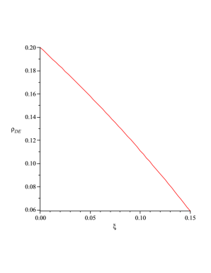
Figure 1: Variation of $\rho_{DE}^{(eff)}$ versus $\xi$ in a $t=constant$ slice.

Figure $2$ shows the variation of the effective dark energy density versus the cosmic time.

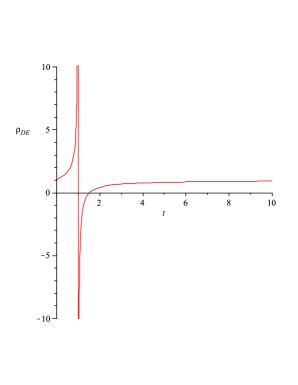
Figure 2: Variation of the effective dark energy density versus the cosmic time. The effective dark energy density increases with time and therefore shows a phantom-like behavior.

As this figure shows, $\rho_{DE}^{eff}$ increases with cosmic time and this is exactly the phantom-like behavior we are interested in. Note that this phantom-like effects is realized without introducing any phantom matter on the brane and only screening of the brane cosmological constant causes such an intriguing effect. Although the existence of a canonical scalar field non-minimally coupled to the induced gravity on the brane has no considerable effect on the phantom-like behavior but as figures $1$ and $3$ show, increasing the values of the non-minimal coupling leads to the reduction of the effective dark energy on a constant time slice. Figure $3$ shows the variation of the effective dark energy versus the cosmic time and non-minimal coupling. We note that while the introduction of a phantom field requires the violation of the null energy condition, here this energy condition is respected since we have not included any phantom matter on the brane. Since the phantom-like dynamics realized in this setup is gravitational ( the quintessence field introduced here plays the role of standard matter on the brane), the null energy condition cannot be violated in this case.

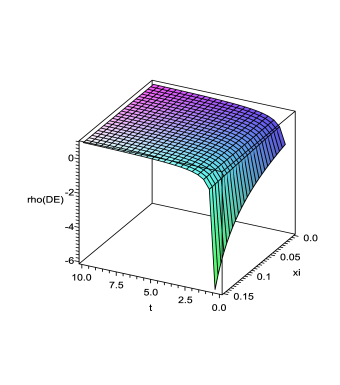
Figure 3: Variation of the effective dark energy versus the cosmic time and the non-minimal coupling. For a constant $\xi$ the model realizes phantom-like effect versus cosmic time.

3 DGP-inspired $F(R,\phi)$ Gravity

3.1 The Setup

Now we extend our previous analysis to the more general case with DGP-inspired $F(R,\phi)$ models. In other words, we incorporate possible modification of the induced gravity on the brane. We assume also a general coupling between a quintessence field localized on the brane and modified induced gravity ( these types of theories have been studied extensively and from various perspectives, see for instance [26, 30, 37]). The action of this model is as follows

$$S=\frac{m_{4}^{3}}{2}\int d^{5}(x)\sqrt{-g}\Re+\int d^{4}(x)\sqrt{-q}\Big{(}\frac{m_{3}^{2}}{2}F(R,\phi)-\frac{1}{2}q^{\mu\nu}\nabla_{\mu}\phi\nabla_{\nu}\phi-V(\phi)+m_{4}^{3}\overline{K}+L_{m}\Big{)},$$ (22)

where the first term shows the usual Einstein-Hilbert action in 5D bulk with 5D metric denoted by $g_{AB}$ and Ricci scalar denoted by $\Re$. The second term on the right is a generalization of the Einstein-Hilbert action induced on the brane. This is an extension of the scalar-tensor theories in one side and a generalization of $f(R)$-gravity on the other side. We call this model as DGP-inspired $F(R,\phi)$ scenario. $y$ is the coordinate of the fifth dimension and we suppose that brane is located at $y=0$ . $q_{\mu\nu}$ is induced metric on the brane which is connected to $g_{AB}$ via $q_{\mu\nu}=\delta_{\mu}\,^{A}\delta_{\nu}\,^{B}g_{AB}$. We denote matter field Lagrangian by $L_{m}=L_{m}(q_{\mu\nu},\psi)+\frac{\Lambda}{8\pi G}$ with energy-momentum tensor defined as $T_{\mu\nu}=-2\frac{\delta L_{m}}{\delta q^{\mu\nu}}+q_{\mu\nu}L_{m}$. The pure scalar field lagrangian is $L_{\phi}=-\frac{1}{2}q^{\mu\nu}\nabla_{\mu}\phi\nabla_{\nu}\phi-V(\phi)$ which gives the following energy-momentum tensor

$$\tau_{\mu\nu}=\nabla_{\mu}{\phi}\nabla_{\nu}\phi-\frac{1}{2}q_{\mu\nu}(\nabla\phi)^{2}-q_{\mu\nu}V(\phi).$$ (23)

The field equations resulting from this action are given as follows

$$\frac{m_{4}^{3}}{F^{\prime}(R,\phi)}\bigg{(}\Re_{AB}-\frac{1}{2}g_{AB}\Re\bigg{)}+m_{3}^{2}\delta_{A}\,^{\mu}\delta_{B}\,^{\nu}\Big{(}R_{\mu\nu}-\frac{1}{2}q_{\mu\nu}R\Big{)}\delta(y)=\delta_{A}\,^{\mu}\delta_{B}\,^{\nu}(\hat{T}_{\mu\nu}+\hat{\tau}_{\mu\nu}+T_{\mu\nu}^{(curv)})\delta(y).$$ (24)

In this relation $\hat{T}_{\mu\nu}\equiv\frac{T_{\mu\nu}}{F^{\prime}(R,\phi)}$ where $T_{\mu\nu}$ is the energy-momentum tensor in matter frame and $\hat{\tau}_{\mu\nu}\equiv\frac{\tau_{\mu\nu}}{F^{\prime}(R,\phi)}$. A prime denotes differentiation with respect to $R$. Also, $T_{\mu\nu}^{(curv)}$ is defined as follows

$$T_{\mu\nu}^{(curv)}=\frac{m_{3}^{2}}{F^{\prime}(R,\phi)}\bigg{[}\frac{1}{2}q_{\mu\nu}\bigg{(}F(R,\phi)-RF^{\prime}(R,\phi)\bigg{)}+\bigg{(}F^{\prime}(R,\phi)\bigg{)}^{;\alpha\beta}\bigg{(}q_{\mu\alpha}q_{\nu\beta}-q_{\mu\nu}q_{\alpha\beta}\bigg{)}\bigg{]}.$$ (25)

In the bulk, $T_{AB}=0$ and therefore

$$G_{AB}=\Re_{AB}-\frac{1}{2}g_{AB}\Re=0$$ (26)

and on the brane we have

$$G_{\mu\nu}=R_{\mu\nu}-\frac{1}{2}q_{\mu\nu}R=\frac{{\cal{T}}_{\mu\nu}}{m_{3}^{2}},$$ (27)

where ${\cal{T}}_{\mu\nu}=\hat{T}_{\mu\nu}+\hat{\tau}_{\mu\nu}+T_{\mu\nu}^{(curv)}$. The corresponding junction conditions relating quantities on the brane are as follows

$$\lim_{\epsilon\longrightarrow+0}[K_{\mu\nu}]_{y=-\epsilon}^{y=+\epsilon}=\frac{F^{\prime}(R,\phi)}{m_{4}^{3}}\bigg{[}{\cal{T}}_{\mu\nu}-\frac{1}{3}q_{\mu\nu}q^{\alpha\beta}{\cal{T}}_{\alpha\beta}\bigg{]}_{y=0}-$$

$$\frac{m_{3}^{2}}{m_{4}^{3}}F^{\prime}(R,\phi)\bigg{[}R_{\mu\nu}-\frac{1}{6}q_{\mu\nu}q^{\alpha\beta}R_{\alpha\beta}\bigg{]}_{y=0}$$ (28)

A detailed study of weak field limit of this scenario within a harmonic gauge on the longitudinal coordinates and using Green’s method to find gravitational potential, leads us to a modified (effective) cross-over distance in this set-up as follows ( see [27] for details of a similar argument)

$$\ell_{F}=\frac{m_{3}^{2}}{2m_{4}^{3}}\bigg{(}\frac{dF}{dR}\bigg{)}=\bigg{(}\frac{dF}{dR}\bigg{)}\ell_{DGP},$$ (29)

where as usual $\ell_{DGP}=\frac{m_{3}^{2}}{2m_{4}^{3}}.$

3.2 Cosmological Implications of the Model

As we have explained in the previous section, embedding of FRW cosmology in DGP setup is possible in the sense that this model accounts for cosmological equations of motion at any distance scale on the brane with any function of the Ricci scalar. To study cosmology of a DGP-inspired $F(R,\phi)$ scenario, we consider the line element as defined in equation (11). Also, we assume that the scalar field $\phi$ depends only on the cosmic time on the brane. Choosing a Gaussian normal coordinate system so that $b^{2}(y,t)=1$, non-vanishing components of the Einstein’s tensor in the bulk plus junction conditions on the brane defined as

$$\lim_{\epsilon\longrightarrow+0}[\partial_{y}n]_{y=-\epsilon}^{y=+\epsilon}(t)=\frac{2nm_{3}^{2}}{m_{4}^{3}}\bigg{[}\Big{(}\frac{dF}{dR}\Big{)}\Big{(}\frac{\ddot{a}}{n^{2}a}-\frac{\dot{a}^{2}}{2n^{2}a^{2}}-\frac{\dot{n}\dot{a}}{n^{3}a}-\frac{k}{2a^{2}}\Big{)}\bigg{]}_{y=0}$$

$$+\frac{n}{3m_{4}^{3}}\bigg{[}\Big{(}\frac{dF}{dR}\Big{)}\Big{(}2\rho^{(tot)}+3p^{(tot)}\Big{)}\bigg{]}_{y=0},$$ (30)

$$\lim_{\epsilon\longrightarrow+0}[\partial_{y}a]_{y=-\epsilon}^{y=+\epsilon}(t)=\frac{m_{3}^{2}}{m_{4}^{3}}\bigg{[}\Big{(}\frac{dF}{dR}\Big{)}\Big{(}\frac{\dot{a}^{2}}{n^{2}a}+\frac{k}{a}\Big{)}\bigg{]}_{y=0}-\bigg{[}\bigg{(}\frac{dF}{dR}\bigg{)}\frac{\rho^{(tot)}a}{3m_{4}^{3}}\bigg{]}_{y=0}$$ (31)

yield the following generalization of the Friedmann equation for cosmological dynamics on the brane ( see [26,27] for machinery of calculations for a simple case)

$$H^{2}+\frac{k}{a^{2}}=\frac{1}{3m_{3}^{2}F^{\prime}(R,\phi)}\Bigg{(}\rho^{tot}+\rho_{0}\bigg{[}1+\epsilon\sqrt{1+\frac{2}{\rho_{0}}\bigg{[}\rho^{tot}-\frac{m_{3}^{2}F^{\prime}(R,\phi)\varepsilon_{0}}{a^{4}}\bigg{]}}\bigg{]}\Bigg{)}$$ (32)

where $\epsilon=\pm 1$ shows two different embedding of the brane,   $\rho_{0}=\frac{6m_{4}^{6}}{m_{3}^{2}F^{\prime}(R,\phi)}$  and  $\varepsilon_{0}=3\Big{(}\frac{\dot{a}^{2}}{n^{2}}-a^{\prime 2}+k\Big{)}a^{2}$  is a constant with respect to $y$ ( with $a^{\prime}\equiv\frac{da}{dy}$) ( see [34,27,38] for more detailed discussion on the constancy of this quantity). Total energy density and pressure are defined as  $\rho^{(tot)}=\hat{\rho}+\rho_{\phi}+\rho^{curv}+\rho_{\Lambda}$  and   $p^{(tot)}=\hat{p}+p_{\phi}+p^{curv}+p_{\Lambda}$  respectively. The ordinary matter on the brane has a perfect fluid form with energy density $\hat{\rho}$ and pressure $\hat{p}$, while the energy density and pressure corresponding to non-minimally coupled quintessence scalar field and also those related to curvature are given as follows

$$\rho_{\varphi}=\bigg{[}\frac{1}{2}\dot{\phi}^{2}+n^{2}V(\phi)-6\frac{dF}{d\phi}H\dot{\phi}\bigg{]}_{y=0},$$ (33)

$$p_{\phi}=\bigg{[}\frac{1}{2n^{2}}\dot{\phi}^{2}-V(\phi)+\frac{2}{n^{2}}\frac{dF}{d\phi}(\ddot{\phi}-\frac{\dot{n}}{n}\dot{\phi})+4\frac{dF}{d\phi}\frac{H}{n^{2}}\dot{\phi}+\frac{2}{n^{2}}\frac{d^{2}F}{d\phi^{2}}\dot{\phi}^{2}\bigg{]}_{y=0}.$$ (34)

also

$$\rho^{(curv)}=\frac{m_{3}^{2}}{F^{\prime}(R,\phi)}\bigg{(}\frac{1}{2}\bigg{[}F(R,\phi)-RF^{\prime}(R,\phi)\bigg{]}-3\dot{R}HF^{\prime\prime}(R,\phi)\bigg{)},$$ (35)

$$p^{(curv)}=\frac{m_{3}^{2}}{F^{\prime}(R,\phi)}\bigg{(}{2\dot{R}HF^{\prime\prime}(R,\phi)+\ddot{R}F^{\prime\prime}(R,\phi)+\dot{R}^{2}F^{\prime\prime\prime}(R,\phi)-\frac{1}{2}\Big{[}F(R,\phi)-RF^{\prime}(R,\phi)\Big{]}}\bigg{)}.$$ (36)

where $H=\frac{\dot{a}(0,t)}{a(0,t)}$  is the Hubble parameter on the brane. Ricci scalar on the brane is given by

$$R=3\frac{k}{a^{2}}+\frac{1}{n^{2}}\bigg{[}6\frac{\ddot{a}}{a}+6\Big{(}\frac{\dot{a}}{a}\Big{)}^{2}-6\frac{\dot{a}}{a}\frac{\dot{n}}{n}\bigg{]}.$$

Note that cosmological dynamics on the brane is given by setting $n(0,t)=1$. With this gauge condition we recover the usual time on the brane via transformation $t=\int^{t}n(0,\eta)\,d\eta$ where $\eta$ is conformal time. It is interesting to note that the equation of state parameter of the scalar field defined as

$$\omega_{\phi}=\frac{\big{(}\frac{1}{2}+2\frac{d^{2}F}{d\phi^{2}}\big{)}\dot{\phi}^{2}-V(\phi)+2\frac{dF}{d\phi}\big{(}\ddot{\phi}+2H\dot{\phi}\big{)}+\frac{m_{3}^{2}}{F^{\prime}(R,\phi)}\big{[}\big{(}2\dot{R}H+\ddot{R}\big{)}F^{\prime\prime}(R,\phi)+\dot{R}^{2}F^{\prime\prime\prime}(R,\phi)-\frac{1}{2}F(R,\phi)+\frac{1}{2}RF^{\prime}(R,\phi)\big{]}}{\frac{1}{2}\dot{\phi}^{2}+V(\phi)-6\frac{dF}{d\phi}H\dot{\phi}+\frac{m_{3}^{2}}{F^{\prime}(R,\phi)}\big{(}\frac{1}{2}F(R,\phi)-\frac{1}{2}RF^{\prime}(R,\phi)-3\dot{R}H\frac{d^{2}F}{dR^{2}}\big{)}},$$ (37)

crosses the phantom-divide line $\omega=-1$ in the favor of recent observations [26,30].

3.3 The Phantom-Like Behavior

Now in this DGP-inspired $F(R,\phi)$ model, the crossover scale takes the following form

$$\ell_{f}=\frac{m_{3}^{2}F^{\prime}(R,\phi)}{2m_{4}^{3}}={F^{\prime}(R,\phi)l_{DGP}},$$ (38)

also

$$\rho_{0}=\frac{3m_{3}^{2}F^{\prime}(R,\phi)}{2\ell_{f}^{2}}.$$

Neglecting the dark radiation term in equation (32), we find

$$H^{2}=\frac{8\pi G(\rho_{m}+\rho_{\phi})}{3}+\frac{\Lambda}{3}+\frac{1}{2\ell_{f}^{2}}+\varepsilon\sqrt{\frac{1}{4\ell_{f}^{4}}+\frac{1}{\ell_{f}^{2}}\Big{[}{\frac{8\pi G(\rho_{m}+\rho_{\phi})}{3}+\frac{\Lambda}{3}}\Big{]}}.$$ (39)

where $G\equiv G_{eff}=\Big{(}8\pi m_{3}^{2}F^{\prime}(R,\phi)\Big{)}^{-1}$ and a prime denotes differentiation with respect to $R$. By adopting the negative sign we find

$$H^{2}=\frac{8\pi G(\rho_{m}+\rho_{\phi})}{3}+\frac{\Lambda}{3}-\frac{\Big{[}F^{\prime}(R,\phi)\Big{]}^{-1}H}{l_{DGP}}.$$ (40)

We can compare this equation with equation (17) to conclude that the screening effect on the cosmological constant is modified as follows

$$\frac{8\pi G}{3}\rho^{eff}_{DE}=\frac{\Lambda}{3}-\frac{\Big{[}F^{\prime}(R,\phi)\Big{]}^{-1}H}{l_{DGP}}$$ (41)

As an important especial case, for $F(R,\phi)=f(R)$ we find the screening effect in a general $f(R)$-gravity

$$\frac{8\pi G}{3}\rho_{DE}^{eff}=\lambda-\frac{\Big{[}f^{\prime}(R)\Big{]}^{-1}H}{\ell_{DGP}}.$$ (42)

Now as an enlightening example, we set for instance

$$F(R,\phi)=\frac{1}{2}(1-\xi\phi^{2})[R-(1-n)\zeta^{2}(R/\zeta^{2})^{n}]\,,$$

where $\zeta$ is a suitably chosen parameter ( see for instance [15] and [26]). With this choice, one recovers the general relativity if $n=1$. For $n\neq 1$, we obtain from equation (40)

$$\frac{8\pi G}{3}\rho_{DE}^{eff}=\frac{\Lambda}{3}-\frac{2H}{\ell_{DGP}(1-\xi\phi^{2})(1-n(1-n)\zeta^{2(1-n)}R^{n-1})}$$ (43)

For spatially flat FRW geometry the Riici scalar is given by

$$R=6\frac{\ddot{a}}{a}+6(\frac{\dot{a}}{a})^{2}.$$ (44)

To have an intuition of phantom-like behavior in this case, we adopt a suitable ansatz so that $a(t)=a_{0}t^{\nu}$ and $\phi(t)=\phi_{0}t^{-\mu}$. We set $\nu=1.2$ and $\mu=0.9$ that are reliable from physical grounds. Figure $4$ shows the variation of $\rho_{eff}^{DE}$ versus $n$ in this DGP-inspired $F(R,\phi)$ model. As we see, phantom-like behavior can be realized for $n\geq 0.73$ and $n\leq-0.60$. In other words, for $-0.6\leq n\leq 0.73$ the effective dark energy in this DGP-inspired $F(R,\phi)$ model has no phantom-like behavior.

Figure 4: Variation of the effective dark energy versus $n$ in a DGP-inspired $F(R,\phi)$ model with $F(R,\phi)=\frac{1}{2}(1-\xi\phi^{2})[R-(1-n)\zeta^{2}(R/\zeta^{2})^{n}]$. Phantom-like behavior can be realized for $n\geq 0.73$ and $n\leq-0.60$.

Figure $5$ shows the variation of the effective dark energy versus $n$ and the non-minimal coupling. By increasing the values of $\xi$, the effective dark energy density reduces but for a fixed value of $\xi$, there is phantom-like effect for appropriate values of $n$.

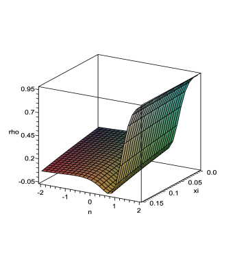
Figure 5: Variation of the effective dark energy versus $n$ and the non-minimal coupling.

Also, figure $6$ shows the variation of the effective dark energy versus $n$ and the cosmic time. The phantom-like effect ( increasing the values of the effective dark energy) can be realized for suitable range of $n$.

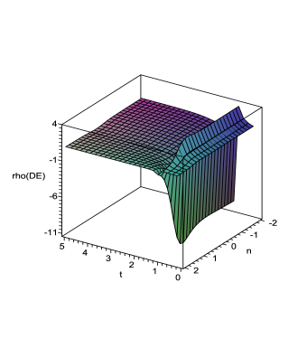
Figure 6: Variation of the effective dark energy versus $n$ and the cosmic time.

3.4 The Expansion History

To investigate expansion history of our model and comparing it with other alternative theories, we study luminosity distance versus redshift in this scenario. For a dark energy model with constant equation of state parameter, the luminosity distance versus redshift can be expressed as follows

$$d_{L}^{\omega}(z)=(1+z)\int_{0}^{z}\frac{H_{0}^{-1}dz}{\bigg{[}\Omega_{M}^{\omega}(1+z)^{3}+(1-\Omega_{M}^{\omega})(1+z)^{3(1+\omega)}\bigg{]}^{1/2}}\,\,,$$ (45)

and for a LCDM model, $\omega=-1$. Now, the evolution of the cosmic expansion in our DGP-inspired $F(R,\phi)$ model is given by

$$\frac{H(z)}{H_{0}}=\frac{1}{2}\Bigg{[}-\frac{1}{r_{0}H_{0}}+\sqrt{\Big{(}2+\frac{1}{r_{0}H_{0}}\Big{)}^{2}+4\Omega_{M}^{0}\Big{[}(1+z)^{3}-1\Big{]}+4\Omega_{\phi}^{0}[(1+z)^{3(1+\omega)}-1]}\,\,\Bigg{]},$$ (46)

where by definition $r_{0}=\ell_{DGP}F^{\prime}(R,\phi)$. The luminosity distance versus redshift in a LDGP model can be expressed as [22]

$$d_{L}^{LDGP}(z)=(1+z)\int_{0}^{z}\frac{dz}{H(z)},$$ (47)

and in our DGP-inspired $F(R,\phi)$ scenario, this quantity denoted as $d_{L}^{FDGP}(z)$ is given by

$$d_{L}^{FDGP}(z)=(1+z)\int_{0}^{z}\frac{dz}{H(z)},$$ (48)

where $H(z)$ is given by equation (46). Figure $7$ shows a comparison between expansion histories of LCDM, LDGP and our FDGP scenario for $F(R,\phi)=\frac{1}{2}(1-\xi\phi^{2})[R-(1-n)\zeta^{2}(R/\zeta^{2})^{n}]$ with $\xi=1/6$ and $n=0.8$. Note that this value of $n$ lies in the appropriate range required for realization of the phantom-like effect obtained in the previous subsection and it is also suitable for describing late-time acceleration ( see for instance the paper by Sotiriou and Faraoni in Ref. [15]). A LCDM scenario has very good agreement with recent observations. As we see here, the FDGP scenario is closer to LCDM more than LDGP. In other words, FDGP has better agreement with recent observation than LDGP. Therefore FDGP provides a better framework for treating phantom-like cosmology without introducing any phantom field. Since we have not introduced any phantom matter on the brane ( $\phi$ is a quintessence field which plays the role of standard matter on the brane), it seems that the null energy condition should be respected in this setup. However, as we will show in subsection $3.6$, this is valid only for some specific values of the model parameters and only in some subspaces of the model parameter space.

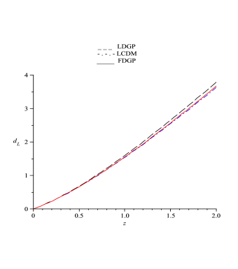
Figure 7: Luminosity distance versus redshift for three alternative scenarios. For a model universe with $F(R,\phi)=\frac{1}{2}(1-\xi\phi^{2})[R-(1-n)\zeta^{2}(R/\zeta^{2})^{n}]$ with $\xi=1/6$ and $n=0.8$, there is better fit between FDGP and LCDM.

3.5 Dynamics of the Equation of State Parameter

To have more detailed discussion on the cosmological dynamics in this model, we find from equation (40) the following relation ( with $8\pi G=1$)

$$H=-\frac{1}{2r_{0}}\Bigg{(}1-\sqrt{1+4r_{0}^{2}\Big{(}\frac{\rho_{m}+\rho_{\phi}}{3}+\frac{\Lambda}{3}\Big{)}}\,\Bigg{)}.$$ (49)

Considering the energy conservation equation which is expressed here as $\dot{\rho}_{tot}+3H(\rho_{tot}+p_{tot})=0$ where $\rho_{tot}=\rho_{m}+\rho_{\phi}$ and $p_{tot}=p_{m}+p_{\phi}$, we find

$$\dot{H}=-\frac{1}{2}\Bigg{[}\rho_{tot}(1+\omega_{tot})-\frac{\dot{F}^{\prime}(R,\phi)}{\ell_{DGP}[F^{\prime}(R,\phi)]^{2}}\Bigg{]}\Bigg{(}1-\frac{1}{\sqrt{1+4[F^{\prime}(R,\phi)]^{2}l_{DGP}^{2}(\frac{\rho_{tot}}{3}+\frac{\Lambda}{3})}}\Bigg{)}.$$ (50)

There is no superacceleration in this DGP-inspired $F(R,\phi)$ scenario if the following condition holds

$$\rho_{tot}\Big{(}1+\omega_{tot}\Big{)}>\frac{\dot{F}^{\prime}(R,\phi)}{\ell_{DGP}[F^{\prime}(R,\phi)]^{2}}.$$ (51)

To have a general relativistic interpretation of the expansion history of this model, we rewrite the energy conservation equation as follows

$$\dot{\rho}_{eff}+3H(1+\omega_{eff})\rho_{eff}=0$$ (52)

and using equation (40) we have

$$\dot{\rho}_{eff}=\frac{-3\Big{[}F^{\prime}(R,\phi)\Big{]}^{-1}\dot{H}}{\ell_{DGP}}+\frac{3H\Big{[}F^{\prime}(R,\phi)\Big{]}^{-2}\dot{F}^{\prime}(R,\phi)}{\ell_{DGP}}.$$ (53)

By comparison of equations (52) and (53), we find

$$1+\omega_{eff}=\frac{\Big{[}F^{\prime}(R,\phi)\Big{]}^{-1}\dot{H}}{H\ell_{DGP}\rho_{eff}}-\frac{\Big{[}F^{\prime}(R,\phi)\Big{]}^{-2}\dot{F}^{\prime}(R,\phi)}{\ell_{DGP}\rho_{eff}}$$ (54)

To realize the phantom phase in this DGP-inspired $F(R,\phi)$ model, the condition $1+\omega_{eff}<0$ should be fulfilled. This leads us to the following condition:

$$\frac{\dot{H}}{H}<\frac{\dot{F}^{\prime}(R,\phi)}{F^{\prime}(R,\phi)}.$$ (55)

It is obvious that this model has the potential to describe the crossing of the phantom divide line.

3.6 The Null Energy Condition

It is important to check the validity of the null energy condition in this setup. In fact, the main feature of this setup is the realization of the phantom-like behavior without introducing any phantom matter on the brane. The null energy condition is respected if the condition $\rho+p>0$ is valid. In our case, this condition is given by $\rho_{tot}+p_{tot}>0$ where $\rho_{tot}$ and $p_{tot}$ are defined in the subsection $3.2$. Figure $8$ shows the variation of $y\equiv(\rho+p)_{tot}$ versus $n$ for some specific values of redshift. As this figure shows, there are appropriate subspaces of the model parameter space that the null energy condition is respected in this setup. This is enough to say that this DGP-inspired $F(R,\phi)$ model realizes the phantom-like behavior without violating the null energy condition, at least in some subspaces of the model parameter space. For instance, at $z=0.25$ ( which is corresponding to the epoch of the phantom-divide line crossing), the null energy condition is respected if $n\leq 1.8$. Albeit, those values of $n$ are adequate that are supported observationally( by, for instance, solar system tests). It should however be noticed that this range seems more restrained at higher redshifts. The reason for violation of the null energy condition in some subspaces of the model parameter space lies in the fact that a modified theory of gravity of the form $f(R)$ is equivalent to a theory of standard gravity plus a scalar field. With $f(R)$ gravity, we have shown that one can mimic a phantom-like behavior without introduction of a phantom field, but when the scenario is written in the Einstein frame, the resulting scalar will violate the null energy condition. So, it is natural to accept that in our model there are some subspaces of the model parameter space that the null energy condition can be violated. The main achievement is however the existence of other subspaces that respect the null energy condition.

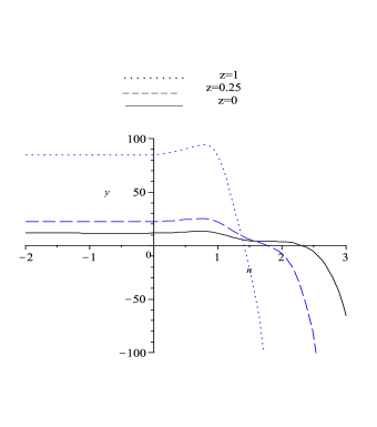
Figure 8: $y\equiv(\rho+p)_{tot}$ versus $n$ for some specific values of redshift. There are some subspaces of the model parameter space that null energy condition is fulfilled for a model universe with $F(R,\phi)=\frac{1}{2}(1-\xi\phi^{2})[R-(1-n)\zeta^{2}(R/\zeta^{2})^{n}]$ with $\xi=1/6$.

4 Summary

Based on the Lue-Starkman conjecture on the dynamical screening of the brane cosmological constant in DGP scenario, in this paper we have extended this proposal to a general DGP-inspired $F(R,\phi)$ Model. Firstly, we have studied phantom-like behavior in the normal branch of an extension of DGP model where a quintessence field is coupled non-minimally to the induced gravity on the brane. The reason for incorporation of this canonical scalar field lies in the fact that without scalar field it is impossible to realize phantom divide line crossing in DGP setup. We have shown that the effective dark energy density decreases by increasing the values of the conformal coupling $\xi$ in a constant cosmic time slice. However, for a constant $\xi$, we have phantom-like behavior ( increasing of the effective dark energy density with cosmic time) in the normal branch of the scenario without introducing any phantom field. Then we have extended our study to a general DGP-inspired $F(R,\phi)$ scenario where we incorporate possible modification of the induced gravity on the brane. In this case we obtained some new and interesting results which we summarize as follows: by adopting the ansatz $F(R,\phi)=\frac{1}{2}(1-\xi\phi^{2})[R-(1-n)\zeta^{2}(R/\zeta^{2})^{n}]\,,$ we have shown that phantom-like behavior can be realized in the normal branch of the scenario if $n\geq 0.73$ and $n\leq-0.60$. In other words, for $-0.6\leq n\leq 0.73$ the effective dark energy in this DGP-inspired $F(R,\phi)$ model has no phantom-like behavior. Investigation of the expansion history of this model shows that this DGP-inspired $F(R,\phi)$ scenario has the best fit with the recent observational data. In fact this model is very close to a LCDM scenario. Finally we found conditions for transition to phantom phase of this model which has the potential to realize phantom divide line crossing. For the case of a quintessence scalar field non-minimally coupled to the induced gravity on the brane, the null energy condition is fulfilled since there is no phantom matter on the brane and the phantom dynamics is essentially gravitational which saves the null energy condition. Also that the brane tension does not violate the null energy condition too. For a general DGP-inspired $F(R,\phi)$ scenario, the null energy condition is respected only in some subspaces of the model parameter space depending on the choice of the model of modified gravity.

Acknowledgement
We would like to thank a referee for his/her important contribution in this work.

References

- [1] S. Perlmutter et al, Astrophys. J. 517 (1999) 565
- [2] A. G. Riess et al, Astron. J. 116 (1998) 1006
- [3] A. D. Miller et al, Astrophys. J. Lett. 524 (1999) L1
- [4] P. de Bernardis et al, Nature 404 (2000) 955
- [5] S. Hanany et al, Astrophys. J. Lett. 545 (2000) L5
- [6] D. N. Spergel et al, Astrophys. J. Suppl. 148 (2003) 175
- [7] L. Page et al, Astrophys. J. Suppl. 148 (2003) 233; G. Hinshaw et al, [WMAP Collaboration], arXiv:0803.0732
- [8] D. N. Spergel et al, Astrophys. J. Suppl. 170 (2007) 377
- [9] G. Hinshaw et al, Astrophys. J. Suppl. 170 (2007) 288
- [10] L. Page et al, Astrophys. J. Suppl. 170 (2007) 335
- [11] A. G. Reiss et al, Astrophys. J 607 (2004) 665; S. W. Allen et al, Mon. Not. R. Astron. Soc. 353 (2004) 457; E. Komatsu et al. [WMAP Collaboration], [arXiv:0803.0547]
- [12] A. A. Andrianov, F. Cannata and A. Y. Kamenshchik, Phys. Rev. D 72 (2005) 043531, [arXiv:gr-qc/0505087].
- [13] E. J. Copeland, M. Sami and S. Tsujikawa, Int. J. Mod. Phys.D 15 (2006) 1753, [ arXiv:hep-th/0603057]
- [14] S. Nesseris, L. Perivolaropoulos, JCAP 0701 (2007) 018
- [15] S. Nojiri and S.D. Odintsov, Int. J. Geom. Meth. Mod. Phys. 4 (2007) 115, [hep-th/0601213]; S. Nojiri and S. D. Odintsov, [arXiv:0807.0685]; T. P. Sotiriou and V. Faraoni, [arXiv:0805.1726]; S. Capozziello and M Francaviglia, Gen. Relativ. Gravit. 40 (2008) 357. See also R. Durrer and R. Maartens, [arXiv:0811.4132]; S. Nojiri and S. D. Odintsov, [arXiv:0807.0685]; K. Bamba, S. Nojiri and S. D. Odintsov, JCAP 0810 (2008) 045, [arXiv:0807.2575]; S. Jhingan, S. Nojiri, S. D. Odintsov, M. Sami, I. Thongkool and S. Zerbini, Phys. Lett.B 663 (2008)424, [ arXiv:0803.2613]
-
[16]
N. Arkani-Hamed, S. Dimopoulos, G. Dvali, Phys. Lett. B 429 (1998) 263
N. Arkani-Hamed, S. Dimopoulos, G. Dvali, Phys. Rev. D 59 (1999) 086004 -
[17]
L. Randall, R. Sundrum, Phys. Rev. Lett. 83 (1999) 3370
L. Randall, R. Sundrum, Phys. Rev. Lett. 83 (1999) 4690 -
[18]
G. Dvali, G. Gabadadze and M. Porrati, Phys. Lett. B 485
(2000) 208
G. Dvali and G. Gabadadze, Phys. Rev. D 63 (2001) 065007
G. Dvali, G. Gabadadze, M. Kolanovi and F. Nitti, Phys. Rev. D 65 (2002) 024031. - [19] H. Zhang and Z.-H. Zhu, Phys. Rev. D 75 (2007) 023510, [arXiv:astro-ph/0611834]. See also K. Nozari, N. Behrouz, T. Azizi and B. Fazlpour, [arXiv:0808.0318]; K. Nozari, M. R. Setare, T. Azizi and N. Behrouz, [ arXiv:0810.1427]
- [20] A. Vikman, Phys. Rev. D 71 (2005) 023515, [astro-ph/0407107]. Y. H. Wei and Y. Z. Zhang, Grav. Cosmol. 9 (2003) 307; Y.H. Wei and Y. Tian, Class. Quantum Grav. 21 (2004) 5347; F. C. Carvalho and A. Saa, Phys. Rev. D 70 (2004) 087302; F. Piazza and S. Tsujikawa, JCAP 0407 (2004) 004; R-G. Cai, H. S. Zhang and A. Wang, Commun. Theor. Phys. 44(2005) 948; I. Y. Arefeva, A. S. Koshelev and S. Y. Vernov, Phys. Rev. D 72 (2005) 064017; A. Anisimov, E. Babichev and A. Vikman, JCAP 0506 (2005)006; B. Wang, Y.G. Gong and E. Abdalla, Phys. Lett. B 624 (2005) 141; S. Nojiri and S. D. Odintsov, hep-th/0506212; S. Nojiri, S. D. Odintsov and S. Tsujikawa, hep-th/0501025; E. Elizalde, S. Nojiri, S. D. Odintsov and P. Wang, Phys. Rev. D 71 (2005) 103504; H. Mohseni Sadjadi, Phys. Rev. D 73 (2006) 063525; W. Zhao and Y. Zhang, Phys. Rev.D 73 (2006)123509; I. Ya. Arefeva and A. S. Koshelev, hep-th/0605085. See also M. Kunz and D. Sapone, Phys. Rev.D 74 (2006) 123503, [arXiv:astro-ph/0609040]
- [21] S. D. Sadatian and K. Nozari, Europhysics Letters, 82 (2008) 49001, K. Nozari and S. D. Sadatian, Eur. Phys. J. C 58 (2008) 499, [arXiv:0809.4744]; K. Nozari and S. D. Sadatian, JCAP 0901 ( 2009) 005, [arXiv:0810.0765]
- [22] A. Lue and G. D. Starkman, Phys. Rev. D 70 (2004) 101501, [arXiv:astro-ph/0408246]
- [23] V. Sahni and Y. Shtanov [arXiv:astro-ph/0202346]; see also V. Sahni [arXiv:astro-ph/0502032]. See also V. Sahni [arXiv:astro-ph/0502032]; Y. Shtanov, V. Sahni, A. Shafieloo and A. Toporensky, JCAP 04 (2009) 023, [arXiv:0901.3074]
- [24] L. P. Chimento, R. Lazkoz, R. Maartens and I. Quiros, JCAP 0609 (2006) 004, [arXiv:astro-ph/0605450]; R. Lazkoz, R. Maartens and E. Majerotto [arXiv:astro-ph/0605701]; R. Maartens and E. Majerotto [arXiv:astro-ph/0603353].
- [25] M. Bouhmadi-Lopez, Nucl. Phys. B 797 (2008) 78-92, [arXiv:astro-ph/0512124]; M. Bouhmadi-Lopez and A. Ferrera, JCAP 0810 (2008) 011, [arXiv:0807.4678]; M. Bouhmadi-Lopez and P. V. Moniz, AIP Conf. Proc. 1122, 201 (2009) [arXiv:0905.4269]; M. Bouhmadi-Lopez, [arXiv:0905.1962]
- [26] K. Nozari and M. Pourghassemi, JCAP 10 (2008) 044, [arXiv:0808.3701]
- [27] K. Nozari, JCAP, 09 (2007) 003, [arXiv:hep-th/07081611]
- [28] M. Sami, [arXiv:0904.3445]
- [29] M. Cadoni and P. Pani, [arXiv:0812.3010]; See also Y. Shtanov, V. Sahni, A. Shafieloo and A. Toporensky, JCAP 04 (2009) 023, [arXiv:0901.3074]
- [30] K. Bamba, C.-Q. Geng, S. Nojiri, S. D. Odintsov, [arXiv:0810.4296]
- [31] V. Faraoni, Phys. Rev. D 62 (2000) 023504
- [32] M. Bouhamdi-Lopez and D. Wands, Phys. Rev. D 71 (2005) 024010
-
[33]
J. W. York, Phys. Rev. Lett. 28 (1972) 1082
G. W. Gibbons and S. W. Hawking, Phys. Rev. D 15 (1977) 2752 - [34] R. Dick, Class. Quant. Grav. 18 (2001) R1, [hep-th/0105320]
- [35] K. Nozari and S. D. Sadatian, Mod. Phys. Lett. A 23(2008) 2933, [arXiv:0710.0058]
- [36] M. Szydlowski, O. Hrycyna and A. Kurek, Phys. Rev. D 77 (2008) 027302, [arXiv:0710.0366]
- [37] G. Barenboim and J. Lykken, JCAP 0803 (2008) 017, [arXiv:0711.3653]
- [38] K. Atazadeh and H. R. Sepangi, Phys. Lett. B 643 (2006) 76, [arXiv:gr-qc/0610107]; K. Atazadeh and H. R. Sepangi, JCAP 0709 (2007) 020, [ arXiv:0710.0214]; K. Atazadeh and H. R. Sepangi, JCAP 01 (2009) 006, [arXiv:0811.3823]; M. Bouhmadi-Lopez, [arXiv:0905.1962].