Convergence of fixed-point continuation algorithms for
matrix rank minimization

Abstract

The matrix rank minimization problem has applications in many fields such as system identification, optimal control, low-dimensional embedding, etc. As this problem is NP-hard in general, its convex relaxation, the nuclear norm minimization problem, is often solved instead. Recently, Ma, Goldfarb and Chen proposed a fixed-point continuation algorithm for solving the nuclear norm minimization problem [33]. By incorporating an approximate singular value decomposition technique in this algorithm, the solution to the matrix rank minimization problem is usually obtained. In this paper, we study the convergence/recoverability properties of the fixed-point continuation algorithm and its variants for matrix rank minimization. Heuristics for determining the rank of the matrix when its true rank is not known are also proposed. Some of these algorithms are closely related to greedy algorithms in compressed sensing. Numerical results for these algorithms for solving affinely constrained matrix rank minimization problems are reported.

June 18, 2009.  This version: December 28, 2010

1 Introduction

In this paper, we are interested in the affinely constrained matrix rank minimization (MRM) problem, which can be cast as

(1.3) $$\begin{array}[]{ll}\min&\mathop{\operator@font rank}\nolimits(X)\\ \mbox{ s.t.}&\mathcal{A}(X)=b,\end{array}$$

where $X\in\mathbb{R}^{{m\times n}}$, $b\in\mathbb{R}^{p}$ and $\mathcal{A}:\mathbb{R}^{{m\times n}}\mapsto\mathbb{R}^{p}$ is a linear map. Without loss of generality, we assume that $m\leq n$ throughout this paper.

Problem (1.3) has applications in many fields such as system identification [32], optimal control [20, 16, 18], and low-dimensional embedding in Euclidean space [30], etc. For example, consider the problem of designing a low-order discrete-time controller for a plant, so that the step response of the combined controller and plant lies within specified bounds. Suppose the plant impulse response is $h(t),t=0,\ldots,N$, the controller impulse response is $x(t),t=0,\ldots,N$, and $u(t)=1,t=0,\ldots,N$ is the step input. Then finding a low-order system is equivalent to solving the following problem:

(1.6) $$\begin{array}[]{ll}\min&\mathop{\operator@font rank}\nolimits(\mathcal{H}(x))\\ \mbox{ s.t.}&b_{l}(t)\leq(h*x*u)(t)\leq b_{u}(t),t=0,\ldots,N,\end{array}$$

where $b_{l}$ and $b_{u}$ are given lower and upper bounds on the step response, $*$ denotes the convolution operator, and $\mathcal{H}(x)$ is the Hankel matrix (see e.g., [17, 39]). Problem (1.6) is an application of an inequality-constrained variant of (1.3).

A special case of (1.3) is the matrix completion problem:

(1.9) $$\begin{array}[]{ll}\min&\mathop{\operator@font rank}\nolimits(X)\\ \mbox{ s.t.}&X_{ij}=M_{ij},\quad\forall(i,j)\in\Omega.\end{array}$$

This problem has applications in online recommendation systems, collaborative filtering [40, 41], etc., including the famous Netflix problem [37]. In the latter problem, users provide ratings to some of the movies in a list of movies. Here $M_{ij}$ is the rating given to $j$-th movie by the $i$-th user. Since users only rate a limited number of movies in the list, we only know some of the entries of the matrix $M$. The goal of the Netflix problem is to fill in the missing entries in this matrix. It is commonly believed that only a few factors contribute to people’s tastes in movies. Thus the matrix $M$ will generally be of low rank. Finding this low-rank completion to $M$ is just the matrix completion problem (1.9).

If $X$ is a diagonal matrix, then (1.3) becomes the compressed sensing problem [8, 12]:

(1.12) $$\begin{array}[]{ll}\min&\|x\|_{0}\\ \mbox{ s.t.}&Ax=b,\end{array}$$

where $A\in\mathbb{R}^{m\times n},b\in\mathbb{R}^{m}$, and $\|x\|_{0}$, which is called the $\ell_{0}$ norm, counts the number of nonzero elements in the vector $x$. The compressed sensing problem, which is currently of great interest in signal processing, is NP-hard [35]. Recent results in compressed sensing have shown that under certain randomness hypotheses, the optimal solution to (1.12) can be found by solving a convex relaxation of (1.12) using only a limited number of measurements. Since the convex envelope of the function $\|x\|_{0}$ on the set $\{x\in\mathbb{R}^{n}:\|x\|_{\infty}\leq 1\}$ is the $\ell_{1}$ norm $\|x\|_{1}:=\sum_{i}|x_{i}|$ [22], a natural choice for a convex relaxation of problem (1.12) is the problem:

(1.15) $$\begin{array}[]{ll}\min&\|x\|_{1}\\ \mbox{ s.t.}&Ax=b.\end{array}$$

Many algorithms for solving (1.12) and (1.15) have been proposed. These include greedy algorithms [42, 13, 45, 14, 36, 11, 1, 2] for (1.12) and convex optimization algorithms [7, 19, 21, 25, 46, 47] for (1.15). See [10] for more information on the theory and algorithms for compressed sensing.

The matrix rank minimization problem (1.3) is also NP-hard. To get a tractable problem, we can replace $\mathop{\operator@font rank}\nolimits(X)$ by the nuclear norm $\|X\|_{*}$ of $X$, the convex envelope of $\mathop{\operator@font rank}\nolimits(X)$ on the set $\{X\in\mathbb{R}^{m\times n}:\|X\|_{2}\leq 1\}$ [38], as proposed by Fazel et al.[16]. The nuclear norm of $X$ is defined as the sum of the nonzero singular values of $X$ and the spectral norm $\|X\|_{2}$ is equal to the largest singular value of $X$; i.e., if the singular values of $X$ are $\sigma_{1}\geq\sigma_{2}\geq\ldots\geq\sigma_{r}>\sigma_{r+1}=\ldots=\sigma_{m}=0,$ then

$$\|X\|_{*}=\sum_{i=1}^{r}\sigma_{i}$$

and $\|X\|_{2}=\sigma_{1}$. Thus, the nuclear norm relaxation of (1.3) is:

(1.18) $$\begin{array}[]{ll}\min&\|X\|_{*}\\ \mbox{ s.t.}&\mathcal{A}(X)=b.\end{array}$$

Let $A$ be the matrix version of $\mathcal{A}$, i.e., $\mathcal{A}(X)=A\cdot\mbox{vec}(X)$, where $\mbox{vec}(X)$ is the vector obtained by stacking the columns of the matrix $X$ in natural order. Recht et al.[38] proved that if the entries of $A$ are drawn from some random distribution and the number of measurements $p\geq Cr(m+n)\log(mn)$, then with very high probability, most $m\times n$ matrices of rank $r$ can be recovered by solving problem (1.18), where $C$ is a positive constant; i.e., an optimal solution to (1.18) gives an optimal solution to (1.3).

If $b$ is contaminated by noise, then (1.18) should be relaxed to

(1.21) $$\begin{array}[]{ll}\min&\|X\|_{*}\\ \mbox{ s.t.}&\|\mathcal{A}(X)-b\|_{2}\leq\theta,\end{array}$$

where $\theta>0$ is the noise level. The Lagrangian version of (1.21) can be written as

(1.22) $$\min\mu\|X\|_{*}+\frac{1}{2}\|\mathcal{A}(X)-b\|_{2}^{2},$$

where $\mu$ is a Lagrangian multiplier.

Several algorithms have been proposed for solving (1.3) and (1.18). Using the fact that (1.18) is equivalent to the semidefinite programming (SDP) problem

(1.26) $$\begin{array}[]{cl}\displaystyle\min_{X,W_{1},W_{2}}&\frac{1}{2}(\mbox{Tr}(W_{1})+\mbox{Tr}(W_{2}))\\ \mbox{ s.t.}&\begin{bmatrix}W_{1}&X\\ X^{\top}&W_{2}\end{bmatrix}\succeq 0,\\ &\mathcal{A}(X)=b,\end{array}$$

where $\mbox{Tr}(W)$ denotes the trace of the square matrix $W$, Recht, Fazel and Parrilo [38] and Liu and Vandenberghe [32] proposed interior-point methods to solve this SDP. However, these interior-point methods cannot be used to solve large problems. First-order methods were proposed by Cai, Candès and Shen [4] and Ma, Goldfarb and Chen [33] that can solve very large matrix rank minimization problems efficiently. One of the algorithms in [33], which is called FPCA (Fixed-Point Continuation with Approximation SVD), almost always achieves the best recoverability. FPCA can recover ${m\times n}$ matrices of rank $r$ using $p$ samples even when $r$ is very close to the largest rank $r_{\max}:=\max\{r|r(m+n-r)/p<1\}$ of ${m\times n}$ matrices that one can recover with only $p$ samples. In this paper, we study the convergence/recoverability properties and numerical performance of FPCA and some of its variants. Our main contribution is a weakening of the conditions previously given by Lee and Bresler [28, 27] required for the approximate recovery of a low-rank matrix.

Notation. We use $\mathbb{R}_{+}^{n}$ to denote the nonnegative orthant of $\mathbb{R}^{n}$. We use $\mathcal{A}^{*}$ to denote the adjoint operator of $\mathcal{A}$. We define the inner product of two matrices $X$ and $Y\in\mathbb{R}^{m\times n}$ to be $\langle X,Y\rangle=\mbox{Tr}(X^{\top}Y)=\mbox{Tr}(Y^{\top}X)$, and denote the Frobenius norm of the matrix $X$ by $\|X\|_{F}=(\mbox{Tr}(X^{\top}X))^{1/2}$ and the Euclidean norm of the vector $x$ by $\|x\|_{2}$. Henceforth, we will write $\mathcal{A}(X)$ as $\mathcal{A}X$ as this should not cause any confusion. For example, $\mathcal{A}^{*}\mathcal{A}X:=\mathcal{A}^{*}(\mathcal{A}(X))$.

Outline. The rest of this paper is organized as follows. In Section 2 we review the role that the restricted isometry property plays in the theory of compressed sensing and matrix rank minimization. We also present three propositions from [28] that provide the basis for the theoretical results that we give later in the paper. We review the Fixed-Point Continuation (FPC) and FPC with Approximate SVD (FPCA) algorithms proposed in [33] in Section 3. We then address the first variant of FPCA, which we call iterative hard thresholding (IHT), and prove convergence results for it in Section 4. Section 5 is devoted to another variant of FPCA, which is called iterative hard thresholding with matrix shrinkage (IHTMS), and convergence results for it. We establish convergence/recoverability properties of FPCAr, a very close variant of FPCA, in Section 6. Some practical issues regarding numerical difficulties and ways to overcome them are discussed in Section 7. Finally, we give some numerical results obtained by applying these algorithms to both randomly created and real matrix rank minimization problems in Section 8.

2 Restricted Isometry Property

In compressed sensing and matrix rank minimization, the restricted isometry property (RIP) of the matrix $A$ or linear operator $\mathcal{A}$ plays a key role in the relationship between the original combinatorial problem and its convex relaxation and their optimal solutions.

The definition of the RIP for matrix rank minimization is:

Definition 1.

For every integer $r$ with $1\leq r\leq m$, the linear operator $\mathcal{A}:\mathbb{R}^{m\times n}\rightarrow\mathbb{R}^{p}$ is said to satisfy the Restricted Isometry Property with the restricted isometry constant $\delta_{r}(\mathcal{A})$ if $\delta_{r}(\mathcal{A})$ is the minimum constant that satisfies

(2.1) $$(1-\delta_{r}(\mathcal{A}))\|X\|_{F}^{2}\leq\|\mathcal{A}X\|_{2}^{2}\leq(1+\delta_{r}(\mathcal{A}))\|X\|_{F}^{2},$$

for all $X\in\mathbb{R}^{m\times n}$ with $\mathop{\operator@font rank}\nolimits(X)\leq r.$ $\delta_{r}(\mathcal{A})$ is called the RIP constant. Note that $\delta_{s}\leq\delta_{t},$ if $s\leq t.$

The RIP concept and the RIP constant $\delta_{r}(\mathcal{A})$ play a central role in the theoretical developments of this paper. We first note that if the operator $\mathcal{A}$ has a nontrivial kernel, i.e., there exists $X\in\mathbb{R}^{m\times n}$ such that $\mathcal{A}X=0$ and $X\neq 0$, then $\delta_{n}(\mathcal{A})\geq 1$. Second, if we represent $\mathcal{A}$ in the coordinate form $(\mathcal{A}X)_{i}=\mbox{Tr}(A_{i}X),i=1,\ldots,p,$ then $\delta_{r}(\mathcal{A})$ is related to the joint kernel of the matrices $A_{i}$. For example, if there exists a matrix $X\in\mathbb{R}^{m\times n}$ with rank $r$ such that $A_{i}X=0,i=1,\ldots,p,$ then $\delta_{r}(\mathcal{A})\geq 1$. Our results in this paper do not apply to such a pathological case.

For matrix rank minimization (1.3), Recht et al.[38] proved the following results.

Theorem 2 (Theorem 3.3 in [38]).

Suppose that $\mathop{\operator@font rank}\nolimits(X)\leq r$, $r\geq 1$ and $\delta_{5r}(\mathcal{A})<0.1$. Then (1.3) and (1.18) have the same optimal solution.

Theorem 3 (Theorem 4.2 in [38]).

Fix $\delta\in(0,1)$. If $\mathcal{A}:\mathbb{R}^{m\times n}\rightarrow\mathbb{R}^{p}$ is a nearly isometric random map (see Definition 4.1 in [38]), then for every $1\leq r\leq m$, there exist constants $c_{0},c_{1}>0$ depending only on $\delta$ such that, with probability at least $1-\exp(-c_{1}p)$, $\delta_{r}(\mathcal{A})\leq\delta$ whenever $p\geq c_{0}r(m+n)\log(mn)$.

Theorems 2 and 3 indicate that if $\mathcal{A}$ is a nearly isometric random map, then with very high probability, $\mathcal{A}$ will satisfy the RIP with a small RIP constant and thus we can solve (1.3) by solving its convex relaxation (1.18). For example, if $A$ is the matrix version of the operator $\mathcal{A}$, and its entries $A_{ij}$ are independent, identically distributed (i.i.d.) Gaussian, i.e., $A_{ij}\sim\mathcal{N}(0,1/p)$, then $\mathcal{A}$ is a nearly isometric random map. For other nearly isometric random maps, see [38].

In Section 8, we will show empirically that when the entries of $A$ are i.i.d. Gaussian, the algorithms proposed in this paper can solve the matrix rank minimization problem (1.3) very well.

It is worth noticing that the linear map $\mathcal{A}$ in the matrix completion problem (1.9) does not satisfy the RIP. A counterexample is given in [5]. For more theory on and algorithms for the matrix completion problem, see [6, 9, 5, 24, 23, 4, 33, 44, 31].

In our proofs of the convergence of FPCA variants, we need $\mathcal{A}$ to satisfy the RIP. Before we describe some properties of the RIP that we will use in our proofs, we need the following definitions.

Definition 4 (Orthonormal basis of a subspace).

Given a set of rank-one matrices $\Psi=\{\psi_{1},\ldots,\psi_{r}\}$, there exists a set of orthonormal matrices $\Gamma=\{\gamma_{1},\ldots,\gamma_{s}\}$, i.e., $\langle\gamma_{i},\gamma_{j}\rangle=0,$ for $i\neq j$ and $\|\gamma_{i}\|_{F}=1$ for all $i$, such that $\mbox{span}(\Gamma)=\mbox{span}(\Psi)$. We call $\Gamma$ an orthonormal basis for the subspace $\mbox{span}(\Psi)$. We use $P_{\Gamma}X$ to denote the projection of $X$ onto the subspace $\mbox{span}(\Gamma).$ Note that $P_{\Gamma}X=P_{\Psi}X$ and $\mathop{\operator@font rank}\nolimits(P_{\Gamma}X)\leq r,\forall X\in\mathbb{R}^{m\times n}.$

Definition 5 (SVD basis of a matrix).

Assume that the rank-$r$ matrix $X_{r}$ has the singular value decomposition $X_{r}=\sum_{i=1}^{r}\sigma_{i}u_{i}v_{i}^{\top}$. $\Gamma:=\{u_{1}v_{1}^{\top},u_{2}v_{2}^{\top},\ldots,u_{r}v_{r}^{\top}\}$ is called an SVD basis for the matrix $X_{r}.$ Note that elements in $\Gamma$ are orthonormal rank-one matrices.

We now list some important properties of linear operators that satisfy RIP.

Proposition 6.

Suppose that the linear operator $\mathcal{A}:\mathbb{R}^{m\times n}\rightarrow\mathbb{R}^{p}$ satisfies the RIP with constant $\delta_{r}(\mathcal{A})$. Let $\Psi$ be an arbitrary orthonormal subset of $\mathbb{R}^{m\times n}$ such that $\mathop{\operator@font rank}\nolimits(P_{\Psi}X)\leq r,\forall X\in\mathbb{R}^{m\times n}$. Then, for all $b\in\mathbb{R}^{p}$ and $X\in\mathbb{R}^{m\times n}$, the following properties hold:

(2.2) $$\|P_{\Psi}\mathcal{A}^{*}b\|_{F}\leq\sqrt{1+\delta_{r}(\mathcal{A})}\|b\|_{2}$$

(2.3) $$(1-\delta_{r}(\mathcal{A}))\|P_{\Psi}X\|_{F}\leq\|P_{\Psi}\mathcal{A}^{*}\mathcal{A}P_{\Psi}X\|_{F}\leq(1+\delta_{r}(\mathcal{A}))\|P_{\Psi}X\|_{F}.$$

Proposition 7.

Suppose that the linear operator $\mathcal{A}:\mathbb{R}^{m\times n}\rightarrow\mathbb{R}^{p}$ satisfies the RIP with constant $\delta_{r}(\mathcal{A})$. Let $\Psi,\Psi^{\prime}$ be arbitrary orthonormal subsets of $\mathbb{R}^{m\times n}$ such that $\mathop{\operator@font rank}\nolimits(P_{\Psi\cup\Psi^{\prime}}X)\leq r$, for any $X\in\mathbb{R}^{m\times n}$. Then the following inequality holds

(2.4) $$\|P_{\Psi}\mathcal{A}^{*}\mathcal{A}(I-P_{\Psi})X\|_{F}\leq\delta_{r}(\mathcal{A})\|(I-P_{\Psi})X\|_{F},\forall X\in\mbox{span}(\Psi^{\prime}).$$

Proposition 8.

If a linear map $\mathcal{A}:\mathbb{R}^{m\times n}\rightarrow\mathbb{R}^{p}$ satisfies

(2.5) $$\|\mathcal{A}X\|_{2}^{2}\leq(1+\delta_{r}(\mathcal{A}))\|X\|_{F}^{2},\quad\forall X\in\mathbb{R}^{m\times n},\mathop{\operator@font rank}\nolimits(X)\leq r,$$

then

(2.6) $$\|\mathcal{A}X\|_{2}\leq\sqrt{1+\delta_{r}(\mathcal{A})}\left(\|X\|_{F}+\frac{1}{\sqrt{r}}\|X\|_{*}\right),\quad\forall X\in\mathbb{R}^{m\times n}.$$

Proofs of Propositions 6, 7 and 8 are given in the Appendix.

3 FPC Revisited

To describe FPC and FPCA and its variants, we need the following definitions.

Definition 9.

Assume that the singular value decomposition of the matrix $X\in\mathbb{R}^{m\times n}$ is given by $X=\sum_{i=1}^{m}\sigma_{i}u_{i}v_{i}^{\top}$ with $\sigma_{1}\geq\sigma_{2}\geq\ldots\geq\sigma_{m}$. Then the best rank-$r$ approximation $R_{r}(X)$ to the matrix $X$ is defined as

$$R_{r}(X)=\sum_{i=1}^{r}\sigma_{i}u_{i}v_{i}^{\top}.$$

$R_{r}:\mathbb{R}^{m\times n}\rightarrow\mathbb{R}^{m\times n}$ is also called the hard thresholding/shrinkage operator with threshold $r$.

Definition 10.

Assume the SVD of the matrix $X$ is given by $X=U\mbox{Diag}(\sigma)V^{\top}$. For $\nu>0$, the matrix shrinkage operator $S_{\nu}(X)$ is defined as

$$S_{\nu}(X)=U\mbox{Diag}((\sigma-\nu)_{+})V^{\top},$$

where $a_{+}:=\max(a,0)$. $S_{\nu}:\mathbb{R}^{m\times n}\rightarrow\mathbb{R}^{m\times n}$ is also called the soft shrinkage operator with threshold $\nu$.

FPC, whose development was motivated by the work on $\ell_{1}$ regularized problems in [21], is based on applying an operator splitting technique to the optimality conditions for (1.22). Note that $X^{*}$ is the optimal solution to (1.22) if and only if

(3.1) $$\mathbf{0}\in\mu\partial\|X^{*}\|_{*}+g(X^{*}),$$

where $g(X^{*})=\mathcal{A}^{*}(\mathcal{A}X^{*}-b)$ is the gradient of the least squares term $\frac{1}{2}\|\mathcal{A}X^{*}-b\|_{2}^{2}$, and $\partial\|X^{*}\|_{*}$ is the subgradient of the nuclear norm $\|X^{*}\|_{*}$ of $X^{*}$. According to [3], the subgradient of $\|X\|_{*}$ is given by

(3.2) $$\partial\|X\|_{*}=\{UV^{\top}+W:U^{\top}W=0,WV=0,\|W\|_{2}\leq 1\},$$

where the SVD of $X$ is given by $X=U\mbox{Diag}(\sigma)V^{\top},U\in\mathbb{R}^{m\times r},V\in\mathbb{R}^{n\times r},\sigma\in\mathbb{R}_{+}^{r}$.

Based on the optimality conditions (3.1), we can develop a fixed-point iterative scheme for solving (1.22) by adopting an operator splitting technique. Note that (3.1) is equivalent to

(3.3) $$\mathbf{0}\in\tau\mu\partial\|X^{*}\|_{*}+X^{*}-(X^{*}-\tau g(X^{*}))$$

for any $\tau>0$. If we let

$$Y^{*}=X^{*}-\tau g(X^{*}),$$

then (3.3) can be rewritten as

(3.4) $$\mathbf{0}\in\tau\mu\partial\|X^{*}\|_{*}+X^{*}-Y^{*},$$

i.e., $X^{*}$ is the optimal solution to

(3.5) $$\min_{X\in\mathbb{R}^{m\times n}}\tau\mu\|X\|_{*}+\displaystyle{\frac{1}{2}}\|X-Y^{*}\|_{F}^{2}.$$

It is known that $S_{\tau\mu}(Y^{*})$ gives the optimal solution to (3.5) [33]. Hence, the following fixed-point iterative scheme can be given for solving (1.22):

(3.8) $$\left\{\begin{array}[]{l}Y^{k+1}=X^{k}-\tau g(X^{k})\\ X^{k+1}=S_{\tau\mu}(Y^{k+1}).\end{array}\right.$$

The following convergence result is proved in [33].

Theorem 11 (Theorem 4 in [33]).

Assume $\tau\in(0,2/\lambda_{max}(\mathcal{A}^{*}\mathcal{A}))$, where $\lambda_{max}(\mathcal{A}^{*}\mathcal{A}))$ denotes the largest eigenvalue of $\mathcal{A}^{*}\mathcal{A}$. The sequence $\{X^{k}\}$ generated by the fixed-point iterations (3.8) converges to some $X^{*}\in\mathcal{X}^{*},$ where $\mathcal{X}^{*}$ is the optimal set of problem (1.22).

Note that in every iteration of (3.8), an SVD has to be computed to perform the matrix shrinkage operation, which is very expensive. Consequently, FPCA uses an approximate SVD to replace the whole SVD, i.e., it computes only a rank-$r$ approximation to $Y^{k+1}$. Note that there are many ways to get a rank-r approximation to $Y^{k+1}$. Here we assume that the best rank-r approximation $R_{r}(Y^{k+1})$ is used. In Section 7, we discuss a Monte Carlo method to approximately compute $R_{r}(Y^{k+1})$, since computing $R_{r}(Y^{k+1})$ exactly is still expensive if $r$ is not very small and the matrices are large. By adopting a continuation strategy for the parameter $\mu$ in (3.8), we arrive at the following FPCA algorithm (Algorithm 1) as proposed in [33].

Initialization: Set $X:=X^{0}$.

for $\mu=\mu_{1},\mu_{2},\ldots,\mu_{L}=\bar{\mu}$ do  while not converged do  $Y:=X-\tau\mathcal{A}^{*}(\mathcal{A}X-b)$.

choose $r$.

$X:=S_{\tau\mu}(R_{r}(Y))$.

   

Algorithm 1 Fixed-Point Continuation with Approximate SVD for MRM (FPCA)

We can see that FPCA makes use of three techniques, hard thresholding, soft shrinkage and continuation. These three techniques have different properties which, when combined, produce a very robust and efficient algorithm with great recoverability properties. By using only one or two of these three techniques, we get different variants of FPCA. We will study two of these variants, Iterative Hard Thresholding (IHT) and Iterative Hard Thresholding with soft Matrix Shrinkage (IHTMS) in Sections 4 and 5, respectively, and FPCA with given rank $r$ (FPCAr) in Section 6.

In the following three sections, we assume that the rank $r$ of the optimal solution is given and we compute the best rank-$r$ approximation to $Y$ in each iteration. In Section 7, we give a heuristic for choosing $r$ in each iteration if $r$ is unknown and use the fast Monte Carlo algorithm proposed in [15] to compute a rank-$r$ approximation to $Y$.

4 Iterative Hard Thresholding

In this section, we study a variant of FPCA that we call Iterative Hard Thresholding (IHT) because of its similarity to the algorithm in [2] for compressed sensing.

If in FPCA, we assume that the rank $r$ is given, we do not do any continuation or soft shrinkage, and always choose the stepsize $\tau$ equal to one, then FPCA becomes Algorithm 2 (IHT). At each iteration of IHT, we first perform a gradient step $Y^{k+1}:=X^{k}-\mathcal{A}^{*}(\mathcal{A}X^{k}-b)$, and then apply hard thresholding to the singular values of $Y^{k+1}$, i.e., we only keep the largest $r$ singular values of $Y^{k+1}$, to get $X^{k+1}$.

Initialization: Given $X^{0},r.$

for k = 0,1,… do  $Y^{k+1}:=X^{k}-\mathcal{A}^{*}(\mathcal{A}X^{k}-b)$.

$X^{k+1}:=R_{r}(Y^{k+1})$

 

Algorithm 2 Iterative Hard Thresholding (IHT)

As previously mentioned, IHT is closely related to an algorithm proposed by Blumensath and Davies [2] for compressed sensing. Their algorithm for solving (1.12) performs the following iterative scheme:

(4.3) $$\left\{\begin{array}[]{l}y^{k+1}=x^{k}-\tau A^{\top}(Ax^{k}-b)\\ x^{k+1}=H_{r}(y^{k+1}),\end{array}\right.$$

where $H_{r}(y)$ is the hard thresholding operator that sets all but the largest (in magnitude) $r$ elements of $y$ to zero. Clearly, IHT for matrix rank minimization and compressed sensing are the same except that the shrinkage operator in the matrix case is applied to the singular values, while in the compressed sensing case it is applied to the solution vector.

To prove the convergence/recoverability properties of IHT for matrix rank minimization, we need the following lemma.

Lemma 12.

Suppose $X:=R_{r}(Y)$ is the best rank-$r$ approximation to the matrix $Y$, and $\Gamma$ is an SVD basis of $X$. Then for any rank-$r$ matrix $X_{r}$ and SVD basis $\Gamma_{r}$ of $X_{r}$, we have

(4.4) $$\|P_{B}X-P_{B}Y\|_{F}\leq\|P_{B}X_{r}-P_{B}Y\|_{F},$$

where $B$ is any orthonormal set of matrices satisfying $\mbox{span}(\Gamma\cup\Gamma_{r})\subseteq\mbox{span}(B)$.

Proof.

Since $X$ is the best rank-$r$ approximation to $Y$ and $rank(X_{r})=r$, $\|X-Y\|_{F}\leq\|X_{r}-Y\|_{F}.$ Hence,

$$\|P_{B}(X-Y)\|_{F}^{2}+\|(I-P_{B})(X-Y)\|_{F}^{2}\leq\|P_{B}(X_{r}-Y)\|_{F}^{2}+\|(I-P_{B})(X_{r}-Y)\|_{F}^{2}.$$

Since $(I-P_{B})X=0$ and $(I-P_{B})X_{r}=0$, this reduces to (4.4). ∎

For IHT, we have the following convergence results, whose proofs essentially follow those given by Blumensath and Davies [2] for IHT for compressed sensing. Our first result considers the case where the desired solution $X_{r}$ satisfies a perturbed linear system of equations $\mathcal{A}X_{r}+e=b$.

Theorem 13.

Suppose that $b=\mathcal{A}X_{r}+e$, where $X_{r}$ is a rank-$r$ matrix, and $\mathcal{A}$ has the RIP with $\delta_{3r}(\mathcal{A})\leq\alpha/\sqrt{8}$ where $\alpha\in(0,1)$. Then, at iteration $k$, IHT will recover an approximation $X^{k}$ satisfying

(4.5) $$\left\|X_{r}-X^{k}\right\|_{F}\leq\alpha^{k}\left\|X_{r}-X^{0}\right\|_{F}+\frac{\beta}{1-\alpha}\|e\|_{2},$$

where $\beta:=2\sqrt{1+\alpha/\sqrt{8}}$. Furthermore, after at most $k^{*}:=\left\lceil\log_{1/\alpha}\left(\left\|X_{r}-X^{0}\right\|_{F}/\|e\|_{2}\right)\right\rceil$ iterations, IHT estimates $X^{r}$ with accuracy

(4.6) $$\left\|X_{r}-X^{k^{*}}\right\|_{F}\leq\frac{1-\alpha+\beta}{1-\alpha}\|e\|_{2}.$$

Proof.

Let $\Gamma_{r}$ and $\Gamma^{k}$ denote SVD bases of $X_{r}$ and $X^{k}$, respectively, and $B_{k}$ denote an orthonormal basis of the subspace $\mbox{span}(\Gamma_{r}\cup\Gamma^{k})$. Let $Z^{k}:=X_{r}-X^{k}$ denote the residual at iteration $k$. Since $P_{B_{k+1}}X_{r}=X_{r}$ and $P_{B_{k+1}}X^{k+1}=X^{k+1}$, it follows first from the triangle inequality and then from Lemma 12 that

(4.7) $$\begin{split}\left\|X_{r}-X^{k+1}\right\|_{F}&\leq\left\|P_{B_{k+1}}X_{r}-P_{B_{k+1}}Y^{k+1}\right\|_{F}+\left\|P_{B_{k+1}}X^{k+1}-P_{B_{k+1}}Y^{k+1}\right\|_{F}\\ &\leq 2\left\|P_{B_{k+1}}X_{r}-P_{B_{k+1}}Y^{k+1}\right\|_{F}.\end{split}$$

Using the fact that $b=\mathcal{A}X_{r}+e$, $Y^{k+1}=X^{k}-\mathcal{A}^{*}(\mathcal{A}X^{k}-\mathcal{A}X_{r}-e)=X^{k}+\mathcal{A}^{*}(\mathcal{A}Z^{k}+e).$ Hence, from (4.7),

$$\begin{split}\left\|X_{r}-X^{k+1}\right\|_{F}&\leq 2\left\|P_{B_{k+1}}X_{r}-P_{B_{k+1}}Y^{k+1}\right\|_{F}\\ &\leq 2\left\|P_{B_{k+1}}X_{r}-P_{B_{k+1}}X^{k}-P_{B_{k+1}}\mathcal{A}^{*}\mathcal{A}(P_{B_{k+1}}Z^{k}+(I-P_{B_{k+1}})Z^{k})-P_{B_{k+1}}\mathcal{A}^{*}e\right\|_{F}\\ &\leq 2\left\|P_{B_{k+1}}Z^{k}-P_{B_{k+1}}\mathcal{A}^{*}\mathcal{A}(P_{B_{k+1}}Z^{k}+(I-P_{B_{k+1}})Z^{k})\right\|_{F}+2\left\|P_{B_{k+1}}\mathcal{A}^{*}e\right\|_{F}\\ &\leq 2\left\|(I-P_{B_{k+1}}\mathcal{A}^{*}\mathcal{A}P_{B_{k+1}})P_{B_{k+1}}Z^{k}\right\|_{F}+2\left\|P_{B_{k+1}}\mathcal{A}^{*}\mathcal{A}(I-P_{B_{k+1}})Z^{k}\right\|_{F}+2\left\|P_{B_{k+1}}\mathcal{A}^{*}e\right\|_{F}.\end{split}$$

Since $\mathop{\operator@font rank}\nolimits(P_{B_{k+1}}X)\leq 2r,\forall X\in\mathbb{R}^{m\times n}$, by applying (2.2) in Proposition 6 we get,

$$\left\|P_{B_{k+1}}\mathcal{A}^{*}e\right\|_{F}\leq\sqrt{1+\delta_{2r}(\mathcal{A})}\|e\|_{2}.$$

Since $P_{\Psi}P_{\Psi}=P_{\Psi}$, it follows from (2.3) in Proposition 6 that the eigenvalues of the linear operator $P_{\Psi}\mathcal{A}^{*}\mathcal{A}P_{\Psi}$ are in the interval $[1-\delta_{r}(\mathcal{A}),1+\delta_{r}(\mathcal{A})]$. Letting $\Psi=B_{k+1}$, it follows that the eigenvalues of $P_{B_{k+1}}\mathcal{A}^{*}\mathcal{A}P_{B_{k+1}}$ lie in the interval $[1-\delta_{2r}(\mathcal{A}),1+\delta_{2r}(\mathcal{A})]$. Hence the eigenvalues of $I-P_{B_{k+1}}\mathcal{A}^{*}\mathcal{A}P_{B_{k+1}}$ are bounded above by $\delta_{2r}(\mathcal{A})$ and it follows that

$$\left\|(I-P_{B_{k+1}}\mathcal{A}^{*}\mathcal{A}P_{B_{k+1}})P_{B_{k+1}}Z^{k}\right\|_{F}\leq\delta_{2r}(\mathcal{A})\left\|P_{B_{k+1}}Z^{k}\right\|_{F}.$$

Also, since $P_{B_{k}}Z^{k}=Z^{k}$, $Z^{k}\in\mbox{span}(B_{k})$ and $\mathop{\operator@font rank}\nolimits(P_{B_{k}\cup B_{k+1}}X)\leq 3r,\forall X\in\mathbb{R}^{m\times n}$, by applying Proposition 7 we get

$$\left\|P_{B_{k+1}}\mathcal{A}^{*}\mathcal{A}(I-P_{B_{k+1}})Z^{k}\right\|_{F}\leq\delta_{3r}(\mathcal{A})\left\|(I-P_{B_{k+1}})Z^{k}\right\|_{F}.$$

Thus, since $\delta_{2r}(\mathcal{A})\leq\delta_{3r}(\mathcal{A})$,

$$\begin{split}\left\|X_{r}-X^{k+1}\right\|_{F}&\leq 2\delta_{2r}(\mathcal{A})\left\|P_{B_{k+1}}Z^{k}\right\|_{F}+2\delta_{3r}(\mathcal{A})\left\|(I-P_{B_{k+1}})Z^{k}\right\|_{F}+2\sqrt{1+\delta_{2r}(\mathcal{A})}\|e\|_{2}\\ &\leq 2\sqrt{2}\delta_{3r}(\mathcal{A})\left\|Z^{k}\right\|_{F}+2\sqrt{1+\delta_{3r}(\mathcal{A})}\|e\|_{2}.\end{split}$$

By assumption, $\delta_{3r}(\mathcal{A})\leq\alpha/\sqrt{8}$; hence we have

(4.8) $$\left\|Z^{k+1}\right\|_{F}\leq\alpha\left\|Z^{k}\right\|_{F}+\beta\|e\|_{2}.$$

Iterating this inequality, we get (4.5).

From (4.5), the recovery accuracy $\left\|Z^{k}\right\|_{F}\leq\frac{1-\alpha+\beta}{1-\alpha}\|e\|_{2}$, if $\alpha^{k}\left\|X_{r}-X^{0}\right\|_{F}\leq\|e\|_{2}$. Hence for $k^{*}:=\left\lceil\log_{1/\alpha}\left(\left\|X_{r}-X^{0}\right\|_{F}/\|e\|_{2}\right)\right\rceil$, (4.6) holds. ∎

Remark 14.

Note that in Theorem 13, convergence is guaranteed for any $\alpha\in(0,1)$. For the choice $\alpha=\frac{1}{2}$, $\beta=2\sqrt{1+1/\sqrt{32}}\approx 2.1696$. Thus (4.5) becomes

$$\left\|X_{r}-X^{k}\right\|_{F}\leq 2^{-k}\left\|X_{r}-X^{0}\right\|_{F}+4.3392\|e\|_{2},$$

and (4.6) becomes

$$\left\|X_{r}-X^{k^{*}}\right\|_{F}\leq 5.3392\|e\|_{2}.$$

For an arbitrary matrix $X$, we have the following result.

Theorem 15.

Suppose that $b=\mathcal{A}X+e$, where $X$ is an arbitrary matrix, and $\mathcal{A}$ has the RIP with $\delta_{3r}(\mathcal{A})\leq\alpha/\sqrt{8}$ where $\alpha\in(0,1)$. Let $X_{r}$ be the best rank-$r$ approximation to $X$. Then, at iteration $k$, IHT will recover an approximation $X^{k}$ satisfying

(4.9) $$\left\|X-X^{k}\right\|_{F}\leq\alpha^{k}\left\|X_{r}-X^{0}\right\|_{F}+\gamma\tilde{\epsilon}_{r},$$

where $\gamma:=\frac{\beta^{2}}{2(1-\alpha)}+1$, $\beta:=2\sqrt{1+\alpha/\sqrt{8}}$, and

(4.10) $$\tilde{\epsilon}_{r}=\left\|X-X_{r}\right\|_{F}+\frac{1}{\sqrt{r}}\left\|X-X_{r}\right\|_{*}+\|e\|_{2},$$

is called the unrecoverable energy (see [36]). Furthermore, after at most $k^{*}:=\left\lceil\log_{1/\alpha}\left(\left\|X_{r}-X^{0}\right\|_{F}/\tilde{\epsilon}_{r}\right)\right\rceil$ iterations, IHT estimates $X$ with accuracy

(4.11) $$\left\|X-X^{k^{*}}\right\|_{F}\leq(1+\gamma)\tilde{\epsilon}_{r}.$$

Proof.

From Theorem 13 with $\tilde{e}=\mathcal{A}(X-X_{r})+e$ instead of $e$, we have

$$\left\|X_{r}-X^{k}\right\|_{F}=\left\|Z^{k}\right\|_{F}\leq\alpha^{k}\left\|X_{r}-X^{0}\right\|_{F}+\frac{\beta}{1-\alpha}\|\tilde{e}\|_{2}.$$

By Proposition 8, we know that

$$\|\tilde{e}\|_{2}\leq\left\|\mathcal{A}(X-X_{r})\right\|_{F}+\|e\|_{2}\leq\sqrt{1+\delta_{r}(\mathcal{A})}\left(\left\|X-X_{r}\right\|_{F}+\frac{1}{\sqrt{r}}\left\|X-X_{r}\right\|_{*}\right)+\|e\|_{2}.$$

Thus we have from the triangle inequality and (4.10)

$$\begin{split}\left\|X-X^{k}\right\|_{F}&\leq\left\|X_{r}-X^{k}\right\|_{F}+\left\|X-X_{r}\right\|_{F}\\ &\leq\alpha^{k}\left\|X_{r}-X^{0}\right\|_{F}+\frac{\beta}{1-\alpha}\|\tilde{e}\|_{2}+\left\|X-X_{r}\right\|_{F}\\ &\leq\alpha^{k}\left\|X_{r}-X^{0}\right\|_{F}+\left(\frac{\beta}{1-\alpha}\sqrt{1+\delta_{r}(\mathcal{A})}+1\right)\tilde{\epsilon}_{r}\\ &\leq\alpha^{k}\left\|X_{r}-X^{0}\right\|_{F}+\gamma\tilde{\epsilon}_{r}.\end{split}$$

This proves (4.9).

Furthermore, $\left\|X-X^{k}\right\|_{F}\leq(1+\gamma)\tilde{\epsilon}_{r}$ if $\alpha^{k}\left\|X_{r}-X^{0}\right\|_{F}\leq\tilde{\epsilon}_{r}$. Therefore, for $k^{*}:=\left\lceil\log_{1/\alpha}\left(\left\|X_{r}-X^{0}\right\|_{F}/\tilde{\epsilon}_{r}\right)\right\rceil$, (4.11) holds. ∎

Remark 16.

For the choice $\alpha=\frac{1}{2}$, $\beta=2\sqrt{1+1/\sqrt{32}}\approx 2.1696$ and $\gamma=\frac{\beta^{2}}{2(1-\alpha)}+1\approx 5.7072$. Thus (4.9) holds as

$$\left\|X-X^{k}\right\|_{F}\leq 2^{-k}\left\|X_{r}-X^{0}\right\|_{F}+5.7072\tilde{\epsilon}_{r},$$

and (4.11) holds as

$$\left\|X-X^{k^{*}}\right\|_{F}\leq 6.7072\tilde{\epsilon}_{r}.$$

Similar bounds on the RIP constant for an approximate recovery were obtained by Lee and Bresler [28, 27] for affinely constrained matrix rank minimization and by Lee and Bresler for ellipsoidally constrained matrix rank minimization [29]. The results in Theorems 13 and 15 improve the previous results for affinely constrained matrix rank minimization in [28, 27]. Specifically, Theorems 13 and 15 require the RIP constant $\delta_{3r}(\mathcal{A})<1/\sqrt{8}\approx 0.3536$, while the result in [28, 27] requires $\delta_{4r}(\mathcal{A})\leq 0.04$ and the result in [29] requires $\delta_{3r}(\mathcal{A})<1/(1+4/\sqrt{3})\approx 0.3022$ for recovery in the noisy case. The IHT algorithm for matrix rank minimization has also been independently studied by Meka, Jain and Dhillon in [34], who have obtained very different results than those in Theorems 13 and 15.

5 Iterative Hard Thresholding with Matrix Shrinkage

We study another variant of FPCA in this section. If in each iteration of IHT, we perform matrix shrinkage to $R_{r}(Y)$ with fixed thresholding $\mu>0$, we get the following algorithm (Algorithm 3), which we call Iterative Hard Thresholding with Matrix Shrinkage (IHTMS). Note that $S_{\mu}(R_{r}(Y))=R_{r}(S_{\mu}(Y)),\forall r,\mu$ and $Y$.

Initialization: Given $X^{0},\mu$ and $r$.

for k = 0,1,… do  $Y^{k+1}:=X^{k}-\mathcal{A}^{*}(\mathcal{A}X^{k}-b)$.

$X^{k+1}:=R_{r}(S_{\mu}(Y^{k+1}))$.

 

Algorithm 3 Iterative Hard Thresholding with Matrix Shrinkage (IHTMS)

For IHTMS, we have the following convergence results.

Theorem 17.

Suppose that $b=\mathcal{A}X_{r}+e$, where $X_{r}$ is a rank-$r$ matrix, and $\mathcal{A}$ has the RIP with $\delta_{3r}(\mathcal{A})\leq\alpha/\sqrt{8}$ where $\alpha\in(0,1)$. Then, at iteration $k$, IHTMS will recover an approximation $X^{k}$ satisfying

(5.1) $$\left\|X_{r}-X^{k}\right\|_{F}\leq\alpha^{k}\left\|X_{r}-X^{0}\right\|_{F}+\frac{1}{1-\alpha}(\beta\|e\|_{2}+2\mu\sqrt{m}),$$

where $\beta:=2\sqrt{1+\alpha/\sqrt{8}}$. Furthermore, after at most $k^{*}:=\left\lceil\log_{1/\alpha}\left(\left\|X_{r}-X^{0}\right\|_{F}/(\|e\|_{2}+2\mu\sqrt{m})\right)\right\rceil$ iterations, IHTMS estimates $X_{r}$ with accuracy

(5.2) $$\left\|X_{r}-X^{k^{*}}\right\|_{F}\leq\frac{1-\alpha+\beta}{1-\alpha}\|e\|_{2}+\frac{2-\alpha}{1-\alpha}2\mu\sqrt{m}.$$

Proof.

Using the same notation as in the proof of Theorem 13, we know that $P_{B_{k+1}}X_{r}=X_{r}$ and $P_{B_{k+1}}X^{k+1}=X^{k+1}$. Using the triangle inequality we get,

(5.3) $$\begin{split}\left\|X_{r}-X^{k+1}\right\|_{F}\leq&\left\|P_{B_{k+1}}X_{r}-P_{B_{k+1}}Y^{k+1}\right\|_{F}\\ &+\left\|P_{B_{k+1}}X^{k+1}-P_{B_{k+1}}S_{\mu}(Y^{k+1})\right\|_{F}\\ &+\left\|P_{B_{k+1}}S_{\mu}(Y^{k+1})-P_{B_{k+1}}Y^{k+1}\right\|_{F}.\end{split}$$

Since $X^{k+1}$ is the best rank-$r$ approximation to $S_{\mu}(Y^{k+1})$, by applying Lemma 12 we get

(5.4) $$\begin{split}\left\|P_{B_{k+1}}X^{k+1}-P_{B_{k+1}}S_{\mu}(Y^{k+1})\right\|_{F}\leq&\left\|P_{B_{k+1}}X_{r}-P_{B_{k+1}}S_{\mu}(Y^{k+1})\right\|_{F}\\ \leq&\left\|P_{B_{k+1}}X_{r}-P_{B_{k+1}}Y^{k+1}\right\|_{F}\\ &+\left\|P_{B_{k+1}}S_{\mu}(Y^{k+1})-P_{B_{k+1}}Y^{k+1}\right\|_{F}.\end{split}$$

Therefore, by combining (5.3), (5.4) and noticing that

$$\left\|P_{B_{k+1}}S_{\mu}(Y^{k+1})-P_{B_{k+1}}Y^{k+1}\right\|_{F}\leq\left\|S_{\mu}(Y^{k+1})-Y^{k+1}\right\|_{F}\leq\mu\sqrt{m},$$

we have

$$\left\|X_{r}-X^{k+1}\right\|_{F}\leq 2\left\|P_{B_{k+1}}X_{r}-P_{B_{k+1}}Y^{k+1}\right\|_{F}+2\mu\sqrt{m}.$$

Using an argument identical the one below (4.7) in the proof of Theorem 13, we get

$$\left\|X_{r}-X^{k+1}\right\|_{F}\leq 2\sqrt{2}\delta_{3r}(\mathcal{A})\left\|Z^{k}\right\|_{F}+2\sqrt{1+\delta_{3r}(\mathcal{A})}\|e\|_{2}+2\mu\sqrt{m}.$$

Now since $\delta_{3r}(\mathcal{A})\leq\alpha/\sqrt{8}$, we have

$$\left\|Z^{k+1}\right\|_{F}\leq\alpha\left\|Z^{k}\right\|_{F}+\beta\|e\|_{2}+2\mu\sqrt{m},$$

which implies that (5.1) holds. Hence (5.2) holds if $k^{*}:=\left\lceil\log_{1/\alpha}\left(\left\|X_{r}-X^{0}\right\|_{F}/(\|e\|_{2}+2\mu\sqrt{m})\right)\right\rceil$. ∎

For an arbitrary matrix $X$, we have the following results.

Theorem 18.

Suppose that $b=\mathcal{A}X+e$, where $X$ is an arbitrary matrix, and $\mathcal{A}$ has the RIP with $\delta_{3r}(\mathcal{A})\leq\alpha/\sqrt{8}$ where $\alpha\in(0,1)$. Let $X_{r}$ be the best rank-$r$ approximation to $X$. Then, at iteration $k$, IHTMS will recover an approximation $X^{k}$ satisfying

(5.5) $$\left\|X-X^{k}\right\|_{F}\leq\alpha^{k}\left\|X_{r}-X^{0}\right\|_{F}+\gamma\tilde{\epsilon}_{r}+\frac{2\mu\sqrt{m}}{1-\alpha},$$

where $\gamma:=\frac{\beta^{2}}{2(1-\alpha)}+1$, $\beta:=2\sqrt{1+\alpha/\sqrt{8}}$, and $\tilde{\epsilon}_{r}$ is defined by (4.10). Furthermore, after at most $k^{*}:=\left\lceil\log_{1/\alpha}\left(\left\|X_{r}-X^{0}\right\|_{F}/(\tilde{\epsilon}_{r}+2\mu\sqrt{m})\right)\right\rceil$ iterations, IHTMS estimates $X$ with accuracy

(5.6) $$\left\|X-X^{k^{*}}\right\|_{F}\leq(1+\gamma)\tilde{\epsilon}_{r}+\frac{2-\alpha}{1-\alpha}2\mu\sqrt{m}.$$

Proof.

The proof of (5.5) is identical to the proof of (4.9) in Theorem 15, except that (5.1) is used instead of (4.5). It also immediately follows from (5.5) that (5.6) holds for $k^{*}:=\left\lceil\log_{1/\alpha}\left(\left\|X_{r}-X^{0}\right\|_{F}/(\tilde{\epsilon}_{r}+2\mu\sqrt{m})\right)\right\rceil$.∎

6 FPCA with Given Rank $r$

In this section, we study the FPCA when rank $r$ is known and a unit stepsize $\tau=1$ is always chosen. This is equivalent to applying a continuation strategy to $\mu$ in IHTMS. We call this algorithm FPCAr (see Algorithm 4 below). The parameter $\eta_{\mu}$ determines the rate of reduction of the consecutive $\mu_{j}$ in continuation, i.e.,

(6.1) $$\mu_{j+1}=\max\{\mu_{j}\eta_{\mu},\bar{\mu}\},j=1,\ldots,L-1$$

For FPCAr, we have the following convergence results.

Input : $X_{(1)}^{0},r,\mu_{1}>\mu_{2}\ldots>\mu_{L}=\bar{\mu}.$

for j = 1,…,L do  Set $\mu=\mu_{j}.$

for k = 0,1,…, until convergence do  $Y_{(j)}^{k+1}:=X_{(j)}^{k}-\mathcal{A}^{*}\left(\mathcal{A}X_{(j)}^{k}-b\right)$.

$X_{(j)}^{k+1}:=S_{\mu}\left(R_{r}\left(Y_{(j)}^{k+1}\right)\right)$.

  Set $X_{(j+1)}^{0}=X_{(j)}^{k+1}.$

  Output : $X^{*}:=X_{(L+1)}^{0}.$

Algorithm 4 FPCA with given rank $r$ (FPCAr)

Theorem 19.

Suppose that $b=\mathcal{A}X_{r}+e$, where $X_{r}$ is a rank-$r$ matrix, and $\mathcal{A}$ has the RIP with $\delta_{3r}(\mathcal{A})\leq\alpha/\sqrt{8}$ where $\alpha\in(0,1)$. Also, suppose in FPCAr, after $K_{j}$ iterations with fixed $\mu=\mu_{j}$, we obtain a solution $X_{(j)}^{(K_{j})}$ that is then set to the initial point $X_{(j+1)}^{0}$ for the next continuation subproblem $\mu=\mu_{j+1}$. Then FPCAr will recover an approximation $X_{(L)}^{(K_{L})}$ that satisfies

(6.2) $$\begin{split}\left\|X_{r}-X_{(L)}^{(K_{L})}\right\|_{F}\leq&\left(\alpha^{\sum_{j=1}^{L}K_{j}}\right)\left\|X_{r}-X^{0}\right\|_{F}+\left(\sum_{j=2}^{L}\alpha^{\sum_{l=j}^{L}K_{l}}+1\right)\frac{\beta}{1-\alpha}\|e\|_{2}\\ &+\left(\sum_{j=2}^{L}\left(\alpha^{\sum_{l=j}^{L}K_{l}}\right)\mu_{j-1}+\mu_{L}\right)\frac{2\sqrt{m}}{1-\alpha},\end{split}$$

where $\beta:=2\sqrt{1+\alpha/\sqrt{8}}$.

Proof.

For $X_{(1)}^{(K_{1})}$, which is obtained by setting $\mu=\mu_{1}$ in the first $K_{1}$ iterations, we get from Theorem 17, that if $\delta_{3r}(\mathcal{A})\leq\alpha/\sqrt{8}$,

(6.3) $$\left\|X_{r}-X_{(1)}^{(K_{1})}\right\|_{F}\leq\alpha^{K_{1}}\left\|X_{r}-X^{0}\right\|_{F}+\frac{\beta}{1-\alpha}\|e\|_{2}+\frac{2\mu_{1}\sqrt{m}}{1-\alpha}.$$

Then from iteration $K_{1}+1$ to $K_{1}+K_{2}$, we fix $\mu=\mu_{2}$. Again by Theorem 17, we get

(6.4) $$\left\|X_{r}-X_{(2)}^{(K_{2})}\right\|_{F}\leq\alpha^{K_{2}}\left\|X_{r}-X_{(1)}^{(K_{1})}\right\|_{F}+\frac{\beta}{1-\alpha}\|e\|_{2}+\frac{2\mu_{2}\sqrt{m}}{1-\alpha}.$$

By substituting (6.3) into (6.4), we get

$$\begin{split}\left\|X_{r}-X_{(2)}^{(K_{2})}\right\|_{F}\leq&\alpha^{(K_{1}+K_{2})}\left\|X_{r}-X^{0}\right\|_{F}+\left(\alpha^{K_{2}}+1\right)\frac{\beta}{1-\alpha}\|e\|_{2}\\ &+\left(\alpha^{K_{2}}\mu_{1}+\mu_{2}\right)\frac{2\sqrt{m}}{1-\alpha}.\end{split}$$

Repeating this procedure we get (6.2). ∎

Theorem 19 shows that as long as $\mu_{L}$ is small and $K_{L}$ is large, the recovery error will be very small. For an arbitrary matrix $X$, we have the following convergence result.

Theorem 20.

Suppose that $b=\mathcal{A}X+e$, where $X$ is an arbitrary matrix. Let $X_{r}$ be the best rank-$r$ approximation to $X$. With the same notation and under the same conditions as in Theorem 19, FPCAr will recover an approximation $X_{(L)}^{(K_{L})}$ that satisfies

$$\begin{split}\left\|X-X_{(L)}^{(K_{L})}\right\|_{F}\leq&\left(\alpha^{\sum_{j=1}^{L}K_{j}}\right)\left\|X_{r}-X^{0}\right\|_{F}+\left(\left(\sum_{j=2}^{L}\alpha^{\sum_{l=j}^{L}K_{l}}+1\right)\gamma+1\right)\tilde{\epsilon}_{r}\\ &+\left(\sum_{j=2}^{L}\left(\alpha^{\sum_{l=j}^{L}K_{l}}\right)\mu_{j-1}+\mu_{L}\right)\frac{2\sqrt{m}}{1-\alpha},\end{split}$$

where $\gamma:=\frac{\beta^{2}}{2(1-\alpha)}+1$, $\beta:=2\sqrt{1+\alpha/\sqrt{8}}$, and $\tilde{\epsilon}_{r}$ is defined by (4.10).

Proof.

We skip the proof here since it is similar to the proof of Theorem 15. ∎

7 Practical Issues

In practice, the rank $r$ of the optimal solution is usually unknown. Thus, in every iteration, we need to determine $r$ appropriately. We propose some heuristics for doing this here. We start with $r:=r_{\max}$. So $X^{1}$ is a rank-$r_{\max}$ matrix. For the $k$-th iteration ( $k\geq 2$ ), $r$ is chosen as the number of singular values of $X^{k-1}$ that are greater than $\epsilon_{s}\sigma_{1}^{k-1}$, where $\sigma_{1}^{k-1}$ is the largest singular value of $X^{k-1}$ and $\epsilon_{s}\in(0,1)$ is a given tolerance. Sometimes the given tolerance truncates too many of the singular values, so we need to increase $r$ occasionally. One way to do this is to increase $r$ by 1 whenever the non-expansive property (see [33]) of the shrinkage operator $S_{\mu}$ is violated some fixed number of times, say 10. In the numerical experiments described in Section 8, we used another strategy; i.e., we increased $r$ by 1 whenever the Frobenius norm of the gradient $g$ increased by more than 10 times. We tested this heuristic for determining $r$ extensively. It enables our algorithms to achieve very good recoverability and appears to be very robust. For many examples, our algorithms can recover matrices whose rank is almost $r_{\max}$ with a limited number of measurements.

Another issue in practice is concerned with the SVD computation. Note that in IHT, IHTMS and FPCA, we need to compute the best rank-$r$ approximation to $Y^{k+1}$ at every iteration. This can be very expensive even if we use a state-of-the-art code like PROPACK [26], especially when the rank of the matrix is relatively large. Therefore, we used instead the Monte Carlo algorithm LinearTimeSVD proposed in [15] to approximate the best rank-$r$ approximation. For a given matrix $A\in\mathbb{R}^{m\times n}$, and parameters $c_{s},k_{s}\in\mathbb{Z}^{+}$ with $1\leq k_{s}\leq c_{s}\leq n$ and $\{p_{i}\}_{i=1}^{n},$ $p_{i}\geq 0,\sum_{i=1}^{n}p_{i}=1$, this algorithm returns approximations $\sigma_{t}(C),t=1,\ldots,k_{s}$ to the largest $k_{s}$ singular values and approximations $H_{k_{s}}^{(t)},t=1,\ldots,k$ to the corresponding left singular vectors of the matrix $A$ in $O(m+n)$ time. Thus, the SVD of $A$ is approximated by

$$A\approx A_{k_{s}}:=H_{k_{s}}\mbox{Diag}(\sigma(C))(A^{\top}H_{k_{s}}\mbox{Diag}(1/\sigma(C))^{\top}.$$

Drineas et al.[15] prove that with high probability, the following estimate holds for both $\xi=2$ and $\xi=F$ when $\{p_{i}\}_{i=1}^{n}$ are nearly optimal probabilities (see [15]):

(7.1) $$\|A-A_{k_{s}}\|_{\xi}^{2}\leq\min_{D:\mathop{\operator@font rank}\nolimits(D)\leq k_{s}}\|A-D\|_{\xi}^{2}+poly(k_{s},1/c_{s})\|A\|_{F}^{2},$$

where $poly(k_{s},1/c_{s})$ is a polynomial in $k_{s}$ and $1/c_{s}$. Thus, $A_{k_{s}}$ is an approximation to the best rank-$k_{s}$ approximation to $A$. The LinearTimeSVD Algorithm, which we found to be much faster than PROPACK, is outlined below in Algorithm 5.

Input : $A\in\mathbb{R}^{m\times n}$, $c_{s},k_{s}\in\mathbb{Z}^{+}$ s.t.$1\leq k_{s}\leq c_{s}\leq n$, $\{p_{i}\}_{i=1}^{n}$ s.t.$p_{i}\geq 0,\sum_{i=1}^{n}p_{i}=1$.

Output : $H_{k}\in\mathbb{R}^{m\times k_{s}}$ and $\sigma_{t}(C),t=1,\ldots,k_{s}.$

for t = 1,…,$c_{s}$ do  Pick $i_{t}\in 1,\ldots,n$ with $Pr[i_{t}=\alpha]=p_{\alpha},\alpha=1,\ldots,n.$

Set $C^{(t)}=A^{(i_{t})}/\sqrt{c_{s}p_{i_{t}}}.$

  Compute $C^{\top}C$ and its SVD; say $C^{\top}C=\sum_{t=1}^{c_{s}}\sigma_{t}^{2}(C)y^{t}{y^{t}}^{\top}.$

Compute $h^{t}=Cy^{t}/\sigma_{t}(C)$ for $t=1,\ldots,k_{s}.$

Return $H_{k_{s}}$, where $H_{k_{s}}^{(t)}=h^{t},$ and $\sigma_{t}(C),t=1,\ldots,k_{s}.$

Algorithm 5 Linear Time Approximate SVD Algorithm [15]

Note that in Algorithm 5, we compute an exact SVD of a smaller matrix $C^{\top}C\in\mathbb{R}^{c_{s}\times c_{s}}$. Thus, $c_{s}$ determines the speed of this algorithm. If we choose a large $c_{s}$, we need more time to compute the SVD of $C^{\top}C$. However, the larger $c_{s}$ is, the more likely are the $\sigma_{t}(C),t=1,\ldots,k_{s}$ to be close to the largest $k_{s}$ singular values of the matrix $A$ since the second term in the right hand side of (7.1) is smaller. In our numerical experiments, we found that we could choose a relatively small $c_{s}$ so that the computational time was reduced without significantly degrading the accuracy. There are many ways to choose the probabilities $p_{i}$. In our numerical experiments in Section 8, we used the simplest one, i.e., we set all $p_{i}$ equal to $1/n$. For other choices of $p_{i}$, see [15] and the references therein.

Although PROPACK is more accurate than this Monte Carlo method (Algorithm 5), we observed from our numerical experiments that our algorithms are very robust and are not very sensitive to the accuracy of the approximate SVDs.

In the $j$-th inner iteration in FPCA we solve problem (1.22) for a fixed $\mu=\mu_{j}$; and stop when

(7.2) $$\frac{\|X^{k+1}-X^{k}\|_{F}}{\max\{1,\|X^{k}\|_{F}\}}<xtol,$$

where $xtol$ is a small positive number. We then decrease $\mu$ and go to the next inner iteration.

8 Numerical Experiments

In this section, we present numerical results for the algorithms discussed above and provide comparisons with the SDP solver SDPT3 [43]. We use IHTr, IHTMSr, FPCAr to denote algorithms in which the rank $r$ is specified, and IHT, IHTMS, FPCA to denote those in which $r$ is determined by the heuristics described in Section 7. We tested these six algorithms on both randomly created and realistic matrix rank minimization problems (1.3). IHTr, IHT, IHTMSr and IHTMS were terminated when (7.2) holds. FPCAr and FPCA were terminated when both (7.2) holds and $\mu_{k}=\bar{\mu}$. All numerical experiments were run in MATLAB 7.3.0 on a Dell Precision 670 workstation with an Intel xeon(TM) 3.4GHZ CPU and 6GB of RAM. All CPU times reported in this section are in seconds.

8.1 Randomly Created Test Problems

We tested some randomly created problems to illustrate the recoverability/convergence properties of our algorithms. The random test problems (1.3) were created in the following manner. We first generated random matrices $M_{L}\in\mathbb{R}^{m\times r}$ and $M_{R}\in\mathbb{R}^{n\times r}$ with i.i.d. Gaussian entries $\sim\mathcal{N}(0,1)$ and then set $M=M_{L}M_{R}^{\top}$. We then created a matrix $A\in\mathbb{R}^{p\times mn}$ with i.i.d. Gaussian entries $A_{ij}\sim\mathcal{N}(0,1/p).$ Finally, the observation $b$ was set equal to $b:=A\mbox{vec}(M)$. We use $SR=p/(mn)$, i.e., the number of measurements divided by the number of entries of the matrix, to denote the sampling ratio. We also list $FR=r(m+n-r)/p$, i.e. the dimension of the set of rank $r$ matrices divided by the number of measurements, in the tables. Note that if $FR>1$, then there is always an infinite number of matrices with rank $r$ satisfying the $p$ linear constraints, so we cannot hope to recover the matrix in this situation. We also report the relative error

$$rel.err.:=\frac{\|X_{opt}-M\|_{F}}{\|M\|_{F}}$$

to indicate the closeness of $X_{opt}$ to $M$, where $X_{opt}$ is the optimal solution to (1.3) produced by our algorithms. We declared $M$ to be recovered if the relative error was less than $10^{-3}.$ We solved 10 randomly created matrix rank minimization problems for each set of $(m,n,p,r)$. We used $NS$ to denote the number of matrices that were recovered successfully. The average time and average relative error of the successfully solved problems are also reported.

The parameters used in the algorithms are summarized in Table 1.

Table 1: Parameters used in the algorithms

parameter	value	description
$\bar{\mu}$	$10^{-8}$	parameter in Algorithms 1 and 4
$\eta_{\mu}$	0.25	parameter in (6.1)
$\epsilon_{s}$	0.01	parameter in LinearTimeSVD
$c_{s}$	$2r_{\max}-2$	parameter in LinearTimeSVD
$p_{i}$	$1/n,\forall i$	parameter in LinearTimeSVD
$xtol$	$10^{-6}$	parameter in (7.2)

We first compare the solvers discussed above that specify the rank $r$ with the SDP solver SDPT3 [43]. The results for a set of small problems with $m=n=60$, 20 percent sampling (i.e., SR = 0.2 and p = 720) and different ranks are presented in Table 2. Note that for this set of parameters $(m,n,p)$, the largest rank that satisfies $FR<1$ is $r_{\max}=6$.

Table 2: Comparison between IHTr, IHTMSr and FPCAr with SDPT3

Prob		SDPT3			IHTr			IHTMSr			FPCAr
r	FR	NS	time	rel.err.	NS	time	rel.err.	NS	time	rel.err.	NS	time	rel.err.
1	0.17	10	122.93	2.31e-10	10	2.60	1.67e-05	10	2.59	1.67e-05	10	4.63	9.00e-06
2	0.33	10	124.26	3.46e-09	10	4.97	1.99e-05	10	4.98	2.11e-05	10	6.06	1.51e-05
3	0.49	3	149.74	2.84e-07	10	10.04	2.38e-05	10	9.95	2.27e-05	10	10.64	2.35e-05
4	0.64	0	—	—	10	22.99	2.88e-05	10	22.72	3.05e-05	10	23.29	2.93e-05
5	0.80	0	—	—	10	75.86	3.89e-05	10	84.13	3.95e-05	10	79.46	3.94e-05

From Table 2 we can see that the performance of our methods is very robust and quite similar in terms of their recoverability properties. They are also much faster and their abilities to recover the matrices are much better than SDPT3. For ranks less than or equal to 5, which is almost the largest rank guaranteeing $FR<1$, IHTr, IHTMSr and FPCAr can recover all randomly generated matrices with a relative error of the order of $1e-5$. However, SDPT3 can only recover all matrices with a rank equal to 1 or 2. When the rank $r$ increases to 3, SDPT3 can only recover 3 of the 10 matrices. When the rank $r$ increases to 4 or 5, none of the 10 matrices can be recovered by SDPT3.

To verify the theoretical results in Sections 4, 5 and 6, we plotted the log of the approximation error $\|X^{k}-X^{*}\|_{F}$ achieved by each of the algorithms IHTr, IHTMSr and FPCAr versus the iteration number $k$ in Figure 1 for one of 10 randomly created problems involving a matrix of rank 2. From this figure, we can see that $\log\|X^{k}-X^{*}\|_{F}$ is approximately a linear function of the iteration number $k$. This implies that our theoretical results in Sections 4, 5 and 6 approximately hold in practice.

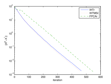
Fig. 1: Approximation error versus the iteration number for a problem where the rank equaled 2

For the same set of test problems, Tables 3, 4, and 5 present comparisons of IHTr versus IHT, IHTMSr versus IHTMS and FPCAr versus FPCA.

Table 3: Comparison between IHTr and IHT

Prob		IHTr			IHT
r	FR	NS	time	rel.err.	NS	time	rel.err.
1	0.17	10	2.60	1.67e-05	10	4.24	1.74e-05
2	0.33	10	4.97	1.99e-05	10	7.00	1.92e-05
3	0.49	10	10.04	2.38e-05	10	13.27	2.32e-05
4	0.64	10	22.99	2.88e-05	10	28.06	2.93e-05
5	0.80	10	75.86	3.89e-05	10	96.32	4.00e-05

Table 4: Comparison between IHTMSr and IHTMS

Prob		IHTMSr			IHTMS
r	FR	NS	time	rel.err.	NS	time	rel.err.
1	0.17	10	2.59	1.67e-05	10	3.98	1.77e-05
2	0.33	10	4.98	2.11e-05	10	6.95	2.04e-05
3	0.49	10	9.95	2.27e-05	10	12.65	2.30e-05
4	0.64	10	22.72	3.05e-05	10	27.12	2.86e-05
5	0.80	10	84.13	3.95e-05	10	94.13	4.10e-05

Table 5: Comparison between FPCAr and FPCA

Prob		FPCAr			FPCA
r	FR	NS	time	rel.err.	NS	time	rel.err.
1	0.17	10	4.63	9.00e-06	10	4.66	8.88e-06
2	0.33	10	6.06	1.51e-05	10	6.15	1.55e-05
3	0.49	10	10.64	2.35e-05	10	11.50	2.24e-05
4	0.64	10	23.29	2.93e-05	10	25.66	2.88e-05
5	0.80	10	79.46	3.94e-05	10	83.91	3.87e-05

From these tables we see that by using our heuristics for determining the rank $r$ at every iteration, algorithms IHT, IHTMS and FPCA perform similarly to algorithms IHTr, IHTMSr and FPCAr which make use of knowledge of the true rank $r$. Specifically, algorithms IHT, IHTMS and FPCA are capable of recovering low-rank matrices very well even when we do not know their rank.

Table 6: Comparison when the given rank is different from the true rank of 3

Given rank	NS	time	rel.err.
IHTr
1	0	—	—
2	0	—	—
3	10	10.04	2.38e-05
4	10	21.42	3.42e-05
5	10	63.53	5.51e-05
6	4	109.00	4.44e-04
IHT	10	13.27	2.32e-05
IHTMSr
1	0	—	—
2	0	—	—
3	10	9.95	2.27e-05
4	10	22.53	3.40e-05
5	10	67.89	5.93e-05
6	1	116.62	6.04e-04
IHTMS	10	12.65	2.30e-05
FPCAr
1	0	—	—
2	0	—	—
3	10	10.64	2.35e-05
4	10	21.26	3.46e-05
5	10	63.67	5.99e-05
6	3	108.02	4.04e-04
FPCA	10	11.50	2.24e-05

Choosing $r$ is crucial in algorithms IHTr, IHTMSr and FPCAr as it is in greedy algorithms for matrix rank minimization and compressed sensing. In Table 6 we present results on how the choice of $r$ affects the performance of algorithms IHTr, IHTMSr and FPCAr when the true rank of the matrix is not known. In Table 6, the true rank is 3 and the results for choices of the rank from 1 to 6 are presented. The rows labeled IHT, IHTMS and FPCA present the results for these algorithms which use the heuristics in Section 7 to determine the rank $r$. From Table 6 we see that if we specify a rank that is smaller than the true rank, then all of the algorithms IHTr, IHTMSr and FPCAr are unable to successfully recover the matrices (i.e., the relative error is greater than 1e-3). Specifically, since for the problems tested the true rank of the matrix was 3, the algorithms failed when $r$ was chosen to be either 1 or 2. If the chosen rank is slightly greater than the true rank (i.e., the rank was chosen to be 4 or 5), all the three algorithms IHTr, IHTMSr and FPCAr still worked. However, the relative errors and times were much worse than those produced by the heuristics based solvers IHT, IHTMS and FPCA. When the chosen rank was too large (i.e., was chosen to be 6), IHTr, IHTMSr and FPCAr were only able to recover the matrices in 4, 1 and 3 out of 10 problems, respectively. However, IHT, IHTMS and FPCA always recovered the matrices.

8.2 A Video Compression Problem

We tested the performance of our algorithms on a video compression problem. By stacking each frame of the video as a column of a large matrix, we get a matrix $M$ whose $j$-th column corresponds to the $j$-th frame of the video. Due to the correlation between consecutive frames of the video matrix, $M$ is expected to be of low rank. Hence we should be able to recover the video by only taking a limited number of measurements. The video used in our experiment was downloaded from the website http://media.xiph.org/video/derf. The original colored video consisted of 300 frames where each frame was an image stored in an RGB format, as a $144\times 176\times 3$ array. Since this video data was too large for our use, we preprocessed it in the following way. We first converted each frame from an RGB format into a grayscale image, so each frame was a $144\times 176$ matrix. We then used only the portion of each frame corresponding to a $39\times 47$ submatrix of pixels in the center of each frame, and took only the first 20 frames. Consequently, the matrix $M$ had $m=1833$ rows and $n=20$ columns. We then created a Gaussian sampling matrix $A\in\mathbb{R}^{p\times(mn)}$ as in Section 8.1 with $p=1833*20*0.4=14664$ rows (i.e., we used sampling ratio $SR=0.4$) and computed $b=A\mbox{vec}(M)\in\mathbb{R}^{p}$. This $14664\times 36660$ matrix $A$ was close to the size limit of what could be created by calling the MATLAB function $A=randn(p,mn)$ on our computer. Although the matrix $M$ was expected to be of low rank, it was only approximately of low rank. Therefore, besides comparing the recovered matrices with the original matrix $M$, we also compared them with the best rank-$5$ approximation of $M$. Since the relative error of the best rank-$5$ approximation of $M$ was $2.33e-2$, we cannot expect to get a more accurate solution. Therefore, we set $xtol$ equal to $0.002$ for this problem. The results of our numerical tests are reported in Table 7. The ranks reported in the table are the ranks of the recovered matrices. The reported relative errors and CPU times are averages over 5 runs. We do not report any results for SDPT3, because the problem is far too large to be solved by an SDP solver. From Table 7 we see that our algorithms were able to recover the matrix $M$ very well, achieving relative errors that were of the same order as that obtained by the best rank-$5$ approximation.

Table 7: Results on recovery of compressed video

Solvers	rank	rel.err.	time
IHTr	5	6.87e-2	645
IHT	5	9.76e-2	949
IHTMSr	5	6.72e-2	688
IHTMS	5	9.69e-2	804
FPCAr	5	5.10e-2	514
FPCA	5	5.17e-2	1296

In Figure 2, the three images in the first column correspond to three particular frames in the original video. The images in the second column correspond to these frames in the rank-$5$ approximation matrix of the video. The images in the third column correspond to these frames in the matrix recovered by FPCA. The other five solvers recovered images that were very similar visually to FPCA so we do not show them here. From Figure 2 we see that FPCA recovers the video very well by taking only 40% as many measurements as there are pixels in the video.

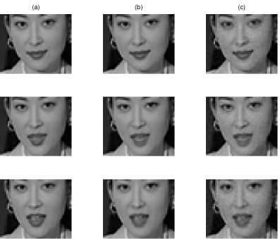
Fig. 2: Comparison of frames 4, 12 and 18 of (a) the original video, (b) the best rank-5 approximation and (c) the matrix recovered by FPCA

Appendix

Here we give proofs of Propositions 6, 7 and 8.

Proof of Proposition 6.

Proof.

We prove (2.2) first. Since for any $X\in\mathbb{R}^{m\times n},$ $\mathop{\operator@font rank}\nolimits(P_{\Psi}X)\leq r$, we have

$$\begin{split}\left|\langle X,P_{\Psi}\mathcal{A}^{*}b\rangle\right|&=|\langle\mathcal{A}P_{\Psi}X,b\rangle|\\ &\leq\|\mathcal{A}P_{\Psi}X\|_{2}\|b\|_{2}\\ &\leq\sqrt{1+\delta_{r}(\mathcal{A})}\|P_{\Psi}X\|_{F}\|b\|_{2}\\ &\leq\sqrt{1+\delta_{r}(\mathcal{A})}\|X\|_{F}\|b\|_{2}.\end{split}$$

Thus

$$\|P_{\Psi}\mathcal{A}^{*}b\|_{F}=\max_{\|X\|_{F}=1}|\langle X,P_{\Psi}\mathcal{A}^{*}b\rangle|\leq\sqrt{1+\delta_{r}(\mathcal{A})}\|b\|_{2}.$$

To prove (2.3), note that by the RIP,

$$(1-\delta_{r}(\mathcal{A}))\|P_{\Psi}X\|_{F}^{2}\leq\|\mathcal{A}P_{\Psi}X\|_{F}^{2}\leq(1+\delta_{r}(\mathcal{A}))\|P_{\Psi}X\|_{F}^{2},$$

which means the eigenvalues of $P_{\Psi}\mathcal{A}^{*}AP_{\Psi}$ restricted to $\mbox{span}(\Psi)$ are in the interval $[1-\delta_{r}(\mathcal{A}),1+\delta_{r}(\mathcal{A})]$. Thus (2.3) holds. $\quad\Box$

Proof of Proposition 7. First, we prove

(A-1) $$\left|\langle\mathcal{A}(I-P_{\Psi})X,\mathcal{A}P_{\Psi}Y\rangle\right|\leq\delta_{r}(\mathcal{A})\|(I-P_{\Psi})X\|_{F}\|P_{\Psi}Y\|_{F},\forall Y\in\mathbb{R}^{m\times n},X\in\mbox{span}(\Psi^{\prime}).$$

(A-1) holds obviously if $(I-P_{\Psi})X=0$ or $P_{\Psi}Y=0$. Thus we can assume $(I-P_{\Psi})X\neq 0$ and $P_{\Psi}Y\neq 0.$ Define $\hat{X}=\frac{(I-P_{\Psi})X}{\|(I-P_{\Psi})X\|_{F}}$ and $\hat{Y}=\frac{P_{\Psi}Y}{\|P_{\Psi}Y\|_{F}}$; then we have $\left\|\hat{X}\right\|_{F}=1$, $\left\|\hat{Y}\right\|_{F}=1$ and $\langle\hat{X},\hat{Y}\rangle=0.$ Since $\hat{X}\in\mbox{span}(\Psi\cup\Psi^{\prime})$ and $\hat{Y}\in\mbox{span}(\Psi)$, we have $\mathop{\operator@font rank}\nolimits\left(\hat{X}+\hat{Y}\right)\leq r$ and $\mathop{\operator@font rank}\nolimits\left(\hat{X}-\hat{Y}\right)\leq r$. Hence by RIP,

$$\begin{split}2(1-\delta_{r}(\mathcal{A}))=(1-\delta_{r}(\mathcal{A}))\left\|\hat{X}+\hat{Y}\right\|_{F}^{2}&\leq\left\|\mathcal{A}\hat{X}+\mathcal{A}\hat{Y}\right\|_{2}^{2}\\ &\leq(1+\delta_{r}(\mathcal{A}))\left\|\hat{X}+\hat{Y}\right\|_{F}^{2}=2(1+\delta_{r}(\mathcal{A})).\end{split}$$

and

$$\begin{split}2(1-\delta_{r}(\mathcal{A}))=(1-\delta_{r}(\mathcal{A}))\left\|\hat{X}-\hat{Y}\right\|_{F}^{2}&\leq\left\|\mathcal{A}\hat{X}-\mathcal{A}\hat{Y}\right\|_{2}^{2}\\ &\leq(1+\delta_{r}(\mathcal{A}))\left\|\hat{X}-\hat{Y}\right\|_{F}^{2}=2(1+\delta_{r}(\mathcal{A})).\end{split}$$

Therefore we have

$$\langle\mathcal{A}\hat{X},\mathcal{A}\hat{Y}\rangle=\frac{\left\|\mathcal{A}\hat{X}+\mathcal{A}\hat{Y}\right\|_{2}^{2}-\left\|\mathcal{A}\hat{X}-\mathcal{A}\hat{Y}\right\|_{2}^{2}}{4}\leq\delta_{r}(\mathcal{A})$$

and

$$-\langle\mathcal{A}\hat{X},\mathcal{A}\hat{Y}\rangle=\frac{\left\|\mathcal{A}\hat{X}-\mathcal{A}\hat{Y}\right\|_{2}^{2}-\left\|\mathcal{A}\hat{X}+\mathcal{A}\hat{Y}\right\|_{2}^{2}}{4}\leq\delta_{r}(\mathcal{A}).$$

Thus, $|\langle\mathcal{A}\hat{X},\mathcal{A}\hat{Y}\rangle|\leq\delta_{r}(\mathcal{A})$ and (A-1) holds.

Finally we have, for any $X\in\mbox{span}(\Psi^{\prime})$,

$$\begin{split}\left\|P_{\Psi}\mathcal{A}^{*}\mathcal{A}(I-P_{\Psi})X\right\|_{F}&=\max_{\|Y\|_{F}=1}|\langle P_{\Psi}\mathcal{A}^{*}\mathcal{A}(I-P_{\Psi})X,Y\rangle|\\ &=\max_{\|Y\|_{F}=1}|\langle\mathcal{A}(I-P_{\Psi})X,\mathcal{A}P_{\Psi}Y\rangle|\\ &\leq\delta_{r}(\mathcal{A})\left\|(I-P_{\Psi})X\right\|_{F},\end{split}$$

i.e., (2.4) holds, which completes the proof. $\quad\Box$

Proof of Proposition 8. This proof essentially follows that given by Needell and Tropp in [36].

Proof.

Let $B^{s}:=\{X\in\mathbb{R}^{m\times n}:\mathop{\operator@font rank}\nolimits(X)=s,\|X\|_{F}\leq 1\}$ be the unit ball of rank-$s$ matrices in $\mathbb{R}^{m\times n}.$ Define the convex hull of the unit norm matrices with rank at most $r$ as:

$$S:=\mbox{conv}\left\{\bigcup_{s\leq r}B^{s}\right\}\subset\mathbb{R}^{m\times n}.$$

By (2.5), we know that the operator norm

$$\|\mathcal{A}\|_{S\rightarrow 2}=\max_{X\in S}\|\mathcal{A}X\|_{2}\leq\sqrt{1+\delta_{r}(\mathcal{A})}.$$

Define another convex set

$$K:=\{X\in\mathbb{R}^{m\times n}:\|X\|_{F}+\frac{1}{\sqrt{r}}\|X\|_{*}\leq 1\}\subset\mathbb{R}^{m\times n},$$

and consider the operator norm

$$\|\mathcal{A}\|_{K\rightarrow 2}=\max_{X\in K}\|\mathcal{A}X\|_{2}.$$

The content of the proposition is the claim that $K\subset S.$

Choose a matrix $X\in K$ with SVD $X=U\mbox{Diag}(\sigma)V^{\top}$. Let $I_{0}$ index the $r$ largest components of $\sigma$, breaking ties lexicographically. Let $I_{1}$ index the next largest $r$ components, and so forth. Note that the final block $I_{J}$ may have fewer than $r$ components. We may assume that $\sigma|_{I_{j}}$ is nonzero for each $j$. This partition induces a decomposition

$$X=U[\mbox{Diag}(\sigma|_{I_{0}})+\sum_{j=1}^{J}\mbox{Diag}(\sigma|_{I_{j}})]V^{\top}=\lambda_{0}Y_{0}+\sum_{j=1}^{J}\lambda_{j}Y_{j},$$

where $\lambda_{j}=\|U\mbox{Diag}(\sigma|_{I_{j}})V^{\top}\|_{F}$ and $Y_{j}=\lambda_{j}^{-1}U\mbox{Diag}(\sigma|_{I_{j}})V^{\top}$. By construction, each matrix $Y_{j}$ belongs to $S$ because it’s rank is at most $r$ and it has unit Frobenius norm. We will prove that $\sum_{j}\lambda_{j}\leq 1,$ which implies that $X$ can be expressed as a convex combination of matrices from the set $S$. So $X\in S$ and $K\subset S.$

Fix $j$ in the range $\{1,2,\ldots,J\}.$ It follows that $\sigma|_{I_{j}}$ contains at most $r$ elements and $\sigma|_{I_{j-1}}$ contains exactly $r$ elements. Therefore,

$$\lambda_{j}=\|\sigma|_{I_{j}}\|_{2}\leq\sqrt{r}\|\sigma|_{I_{j}}\|_{\infty}\leq\sqrt{r}\cdot\frac{1}{r}\|\sigma|_{I_{j-1}}\|_{1}.$$

Summing these relations, we obtain,

$$\sum_{j=1}^{J}\lambda_{j}\leq\frac{1}{\sqrt{r}}\|\sigma|_{I_{j-1}}\|_{1}\leq\frac{1}{\sqrt{r}}\|X\|_{*}.$$

It is obvious that $\lambda_{0}=\|\sigma|_{I_{0}}\|_{2}\leq\|X\|_{F}.$ We now conclude that

$$\sum_{j=0}^{J}\lambda_{j}\leq\|X\|_{F}+\frac{1}{\sqrt{r}}\|X\|_{*}\leq 1$$

because $X\in K.$ This implies that $X\in S$ and $K\subset S$, and thus completes the proof. $\quad\Box$

References

• [1] Blumensath, T., and Davies, M.Β E. Gradient pursuits. IEEE Transactions on Signal Processing 56, 6 (2008), 2370–2382.
• [2] Blumensath, T., and Davies, M.Β E. Iterative hard thresholding for compressed sensing. Applied and Computational Harmonic Analysis 27, 3 (2009), 265–274.
• [3] Borwein, J.Β M., and Lewis, A.Β S. Convex Analysis and Nonlinear Optimization. Springer-Verlag, 2003.
• [4] Cai, J., CandΓ¨s, E.Β J., and Shen, Z. A singular value thresholding algorithm for matrix completion. SIAM J. on Optimization 20, 4 (2010), 1956–1982.
• [5] CandΓ¨s, E.Β J., and Plan, Y. Matrix completion with noise. Proceedings of the IEEE (2009).
• [6] CandΓ¨s, E.Β J., and Recht, B. Exact matrix completion via convex optimization. Foundations of Computational Mathematics 9 (2009), 717–772.
• [7] CandΓ¨s, E.Β J., and Romberg, J. $\ell_{1}$-MAGIC: Recovery of sparse signals via convex programming. Tech. rep., Caltech, 2005.
• [8] CandΓ¨s, E.Β J., Romberg, J., and Tao, T. Robust uncertainty principles: Exact signal reconstruction from highly incomplete frequency information. IEEE Transactions on Information Theory 52 (2006), 489–509.
• [9] CandΓ¨s, E.Β J., and Tao, T. The power of convex relaxation: near-optimal matrix completion. IEEE Trans. Inform. Theory 56, 5 (2009), 2053–2080.
• [10] compressedΒ sensing website, R. http://dsp.rice.edu/cs.
• [11] Dai, W., and Milenkovic, O. Subspace pursuit for compressive sensing signal reconstruction. IEEE Trans. on Information Theory 55, 5 (2009), 2230–2249.
• [12] Donoho, D. Compressed sensing. IEEE Transactions on Information Theory 52 (2006), 1289–1306.
• [13] Donoho, D., Tsaig, Y., Drori, I., and Starck, J.-C. Sparse solution of underdetermined linear equations by stagewise orthogonal matching pursuit. Tech. rep., Stanford University, 2006.
• [14] Donoho, D.Β L., and Tsaig, Y. Fast solution of $\ell_{1}$-norm minimization problems when the solution may be sparse. IEEE Transactions on Information Theory 54, 11 (2008), 4789–4812.
• [15] Drineas, P., Kannan, R., and Mahoney, M.Β W. Fast Monte Carlo algorithms for matrices ii: Computing low-rank approximations to a matrix. SIAM J. Computing 36 (2006), 158–183.
• [16] Fazel, M., Hindi, H., and Boyd, S. A rank minimization heuristic with application to minimum order system approximation. In Proceedings of the American Control Conference (2001), vol.Β 6, pp.Β 4734–4739.
• [17] Fazel, M., Hindi, H., and Boyd, S. Log-det heuristic for matrix rank minimization with applications to Hankel and Euclidean distance matrices. In Proceedings of the American Control Conference (2003), pp.Β 2156–2162.
• [18] Fazel, M., Hindi, H., and Boyd, S. Rank minimization and applications in system theory. In American Control Conference (2004), pp.Β 3273–3278.
• [19] Figueiredo, M. A.Β T., Nowak, R.Β D., and Wright, S.Β J. Gradient projection for sparse reconstruction: Application to compressed sensing and other inverse problems. IEEE Journal on Selected Topics in Signal Processing 1, 4 (2007).
• [20] Ghaoui, L.Β E., and Gahinet, P. Rank minimization under LMI constraints: A framework for output feedback problems. In Proceedings of the European Control Conference (1993).
• [21] Hale, E.Β T., Yin, W., and Zhang, Y. Fixed-point continuation for $\ell_{1}$-minimization: Methodology and convergence. SIAM Journal on Optimization 19, 3 (2008), 1107–1130.
• [22] Hiriart-Urruty, J.-B., and LemarΓ©chal, C. Convex Analysis and Minimization Algorithms II: Advanced Theory and Bundle Methods. Springer-Verlag, New York, 1993.
• [23] Keshavan, R.Β H., Montanari, A., and Oh, S. Matrix completion from noisy entries. arxiv:0906.2027 (2009).
• [24] Keshavan, R.Β H., Montanari, A., and Oh, S. Matrix completion from a few entries. IEEE Trans. on Info. Theory 56 (2010), 2980–2998.
• [25] Kim, S.Β J., Koh, K., Lustig, M., Boyd, S., and Gorinevsky, D. A method for large-scale $\ell_{1}$-regularized least-squares. IEEE Journal on Selected Topics in Signal Processing 4, 1 (2007), 606–617.
• [26] Larsen, R.Β M. PROPACK - software for large and sparse SVD calculations. Available from http://sun.stanford.edu/$\sim$rmunk/PROPACK.
• [27] Lee, K., and Bresler, Y. ADMIRA: atomic decomposition for minimum rank approximation. ArXiv preprint: arXiv:0905.0044 (2009).
• [28] Lee, K., and Bresler, Y. Efficient and guaranteed rank minimization by atomic decomposition. preprint, available at arXiv: 0901.1898v1 (2009).
• [29] Lee, K., and Bresler, Y. Guaranteed minimum rank approximation from linear observations by nuclear norm minimization with an ellipsoidal constraint. Arxiv preprint arXiv:0903.4742 (2009).
• [30] Linial, N., London, E., and Rabinovich, Y. The geometry of graphs and some of its algorithmic applications. Combinatorica 15 (1995), 215–245.
• [31] Liu, Y., Sun, D., and Toh, K.-C. An implementable proximal point algorithmic framework for nuclear norm minimization. preprint, National University of Singapore (2009).
• [32] Liu, Z., and Vandenberghe, L. Interior-point method for nuclear norm approximation with application to system identification. SIAM Journal on Matrix Analysis and Applications 31, 3 (2009), 1235–1256.
• [33] Ma, S., Goldfarb, D., and Chen, L. Fixed point and Bregman iterative methods for matrix rank minimization. To appear in Mathematical Programming Series A (2009). (published online: 23 September 2009).
• [34] Meka, R., Jain, P., and Dhillon, I.Β S. Guaranteed rank minimization via singular value projection. Arxiv preprint, available at http://arxiv.org/abs/0909.5457 (2009).
• [35] Natarajan, B.Β K. Sparse approximate solutions to linear systems. SIAM Journal on Computing 24 (1995), 227–234.
• [36] Needell, D., and Tropp, J.Β A. CoSaMP: Iterative signal recovery from incomplete and inaccurate samples. Applied and Computational Harmonic Analysis 26 (2009), 301–321.
• [37] prize website., N. http://www.netflixprize.com/.
• [38] Recht, B., Fazel, M., and Parrilo, P. Guaranteed minimum-rank solutions of linear matrix equations via nuclear norm minimization. SIAM Review 52, 3 (2010), 471–501.
• [39] Sontag, E. Mathematical Control theory. Springer-Verlag, New York, 1998.
• [40] Srebro, N. Learning with Matrix Factorizations. PhD thesis, Massachusetts Institute of Technology, 2004.
• [41] Srebro, N., and Jaakkola, T. Weighted low-rank approximations. In Proceedings of the Twentieth International Conference on Machine Learning (ICML-2003) (2003).
• [42] Tibshirani, R. Regression shrinkage and selection via the lasso. Journal Royal Statistical Society B 58 (1996), 267–288.
• [43] Toh, K.-C., Todd, M.Β J., and TΓΌtΓΌncΓΌ, R.Β H. SDPT3 - a Matlab software package for semidefinite programming. Optimization Methods and Software 11 (1999), 545–581.
• [44] Toh, K.-C., and Yun, S. An accelerated proximal gradient algorithm for nuclear norm regularized least squares problems. Pacific J. Optimization 6 (2010), 615–640.
• [45] Tropp, J. Just relax: Convex programming methods for identifying sparse signals. IEEE Transactions on Information Theory 51 (2006), 1030–1051.
• [46] vanΒ den Berg, E., and Friedlander, M.Β P. Probing the Pareto frontier for basis pursuit solutions. SIAM J. on Scientific Computing 31, 2 (2008), 890–912.
• [47] Yin, W., Osher, S., Goldfarb, D., and Darbon, J. Bregman iterative algorithms for $\ell_{1}$-minimization with applications to compressed sensing. SIAM Journal on Imaging Sciences 1, 1 (2008), 143–168.