The UV-Excess survey of the Northern Galactic Plane
(UVEX)

Abstract

The UV-Excess Survey of the Northern Galactic Plane images a 10^∘$\times$185^∘ wide band, centered on the Galactic Equator using the 2.5m Isaac Newton Telescope in four bands ($U,g,r,He$i$5875$) down to $\sim$21^st-22^nd magnitude ($\sim$20^th in $He$i$5875$). The setup and data reduction procedures are described. Simulations of the colours of main-sequence stars, giant, supergiants, DA and DB white dwarfs and AM CVn stars are made, including the effects of reddening. A first look at the data of the survey (currently 30% complete) is given.

1 Introduction

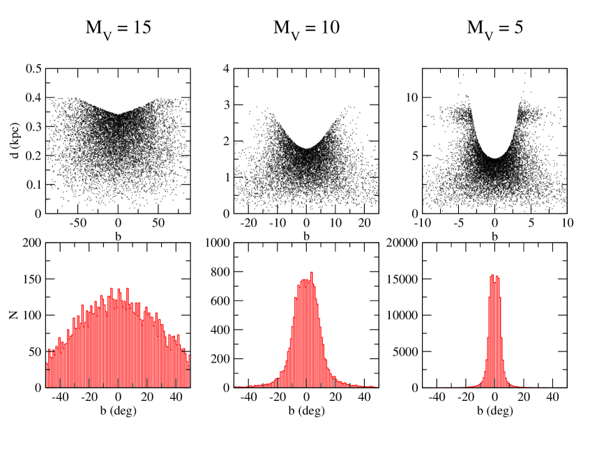
Figure 1: Distribution as a function of heliocentric distance vs. latitude (upper panels) and a histrogram of number of systems vs. latitude (lower panels) of three Galactic populations with absolute visual magnitudes M_V = 15, 10 and 5 (left to right), based on a Galaxy model according to Boissier &Prantzos (1999), and including a Sandage (1972) extinction model, as detailed in Nelemans et al. (2004). A sample with limiting magnitude $V$ = 23 is shown here to illustrate the strong concentration of these populations towards the Galactic Plane. In the M_V = 5 panel the extra sources at $d$ = 8kpc are caused by the Galactic Bulge.

The availability of wide field CCD camera arrays on medium-sized telescopes has led to the emergence of large scale optical surveys of the sky, targeting one or more scientific objectives. The vast majority of these surveys, such as the Sloan Digital Sky Survey (York et al. 2001) are concentrated on the extragalactic universe. However, there is an increasing interest in a more detailed study of our own Milky Way Galaxy as well. The recently completed SDSS-II/SEGUE program (Yanny, Rockosi, Newberg et al., 2009) is specifically targeting lower galactic latitudes, and the RAVE survey (Steinmetz et al., 2006) is targeting the Galactic halo and streams and companions to the Milky Way.

Figure 2: Filter efficiency curves of the $U$, $g$, $r$, $He$i$5875$, $H\alpha$ and $i$ band filters used in the UVEX and IPHAS surveys (dashed and dashed-dotted curves), overplotted onto the spectrum of Vega (solid curve), together with the CCD efficiency curve (dashed).

The plane of the Milky Way, however, has so far not been the target of a full scale optical, multicolour, digital and photon-noise limited survey, despite its obvious value for many fields of astrophysics. This situation is changing with the European Galactic Plane Surveys (EGAPS) currently underway. Combined, the EGAPS surveys (described below) will cover the full Galactic Plane in a strip of 10$\times$360 degrees centred on the Galactic equator, in the $u/U,g,r,i$, $H\alpha$ bands down to (Vega) magnitude $\sim$21 - 22 (or equivalent line flux), and for the Northern survey also in the $He$i$5875$ filter. EGAPS started off with the INT Photometric H$\alpha$ Survey (IPHAS ; Drew et al., 2005, hereafter D05) that covers the Northern Galactic Plane in the $r,i$ and $H\alpha$ bands. Here we describe the UVEX survey: the UV-Excess Survey of the Northern Galactic Plane that uses the exact same set-up as IPHAS but will image the Northern Plane in $U,g,r$ and $He$i$5875$. The Southern Galactic Plane will be covered by the VPHAS+ survey (using $u,g,r,i,H\alpha$) as an ESO Public Survey on the VST+Omegacam combination and will probably start in the beginning of 2010.

Very few dedicated blue surveys at low galactic latitudes exist, apart from all-sky surveys such as the Palomar sky surveys or the ESO sky surveys, performed in the 1950-1990s, using photographic plates. A notable exception is the Sandage Two-Color survey of the Galactic Plane as presented in a series of papers by Lanning (1973) and Lanning & Meakes (2004; and references therein; also see Lanning & Lépine, 2006). The total survey covers 5332 square degrees (124 plates) centered on the Galactic Plane (at $b$ = –6^∘, 0^∘and +6^∘) using photographic plates (6.6 degrees on a side) and the UG1 (‘UV’) and GG13 (‘B’) filters on the Palomar 48-inch Oschin Schmidt telescope. So far 734 UV-bright sources in 39% of the total area of the survey have been published, averaging one source per 2.83 square degrees down to $m_{B}\sim$ 20. UV-bright candidates were selected by eye as having $U-B<0$, but with significant scatter on both the photometry and the completeness due to crowding and differing quality of the photographic plates. Not being digital, and the extra problems crowding present to photographic observations, make the survey good for picking out the bluest objects, but not useful for a systematic study of stellar populations in the Galactic Plane. Although UVEX will cover a smaller area (1850 square degrees for the Northern Survey; 3600 square degrees when ultimately combined with VPHAS+), the survey is fully photometric, allowing a more consistent and more detailed source extraction and all data will be digitally available. First results on the selection of UV-bright sources in UVEX shows a much higher surface density of sources ($\sim$10 per square degree), which is both due to the greater depth of UVEX (in particular in the $g$-band), as well as the more consistent and automated selection techniques, which allow identification of UV-bright objects at a much redder cut-off than was possible for the Sandage Two-Color survey (see Groot et al., 2009, in preparation).

Here we describe the scientific objectives of the UVEX survey (Sect. 2), the survey design and observing strategy (Sect. 3), simulations of stellar populations in the UVEX colours (Sect. 4), the early results (Sect. 5), the seeing statistics and the effect of crowding on the detected number counts (Sect. 6) and conclusions (Sect. 7).

2 Science goals

Figure 3: Magnitude errors for the observations in the four different filters as function of magnitude, as detected in CCD4 of field 6160 taken under median seeing conditions. Note that the Hei data is applicable for the 120 second integrations. After the first year the depth in Hei is increaded by an enlarged integration time (180 seconds).

The main science goal of UVEX is to chart the Galactic population of stellar remnants, single and in binary systems. These include single and binary white dwarfs, subdwarf B stars, Cataclysmic Variables, AM CVn stars and neutron star and black hole binaries. These systems are hot, and therefore blue, due to the remnant energy in the compact objects or they are being kept hot due to accretion. Due to their small size (typically $\mathrel{\hbox{\hbox to0.0pt{\lower 2.36806pt\hbox{$\sim$}\hss} \kern-3.00003pt\raise 1.72218pt\hbox{$<$}}}$1 $R_{\odot}$) these systems are intrinscically faint, despite their hot temperature. In particular, they have much lower absolute visual magnitudes than main sequence stars of similar colours. At a given apparent magnitude they will therefore be much closer by than main sequence stars and therefore have suffered much less extinction than a main sequence star of the same intrinsic colour. This technique to identify stellar remnants has been used before, e.g. to search for old halo white dwarfs in front of molecular clouds (Hodgkin et al. priv.com.). The reason to survey the Galactic Plane is that the target populations are Galactic populations and therefore strongly concentrated towards the Galactic Plane. Fig. 1 illustrates this point. Here we have taken a model of the Galaxy according to the prescription of Boissier & Prantzos (1999), and populated this with populations having absolute visual magnitudes of M_V = 15, 10 and 5. A Sandage (1972) type model of Galactic extinction was included. This Galaxy model is identical to the one used and described more extensively in Nelemans, Yungelson & Portegies Zwart (2004). A limiting magnitude of $V$ = 23 was taken to construct Fig. 1. It can be seen that any population with an absolute magnitude in the range 5$\leq M_{V}\leq$10 is strongly concentrated to the Plane of the Galaxy. Respectively 12%, 40% and 97% of all objects in Fig. 1 lie within the first 5^∘ of the Plane (the limits of the UVEX survey) for $M_{V}$ = 15, 10 and 5. Subdwarf B stars, Cataclysmic Variables, AM CVn stars, young white dwarfs and most neutron star and black hole binaries all have absolute magnitudes $M_{V}<$ 15. It is only for the faintest systems (old white dwarfs and very low mass accretion rate interacting binaries) that we sample such a local population that no concentration towards the Galactic plane is seen.

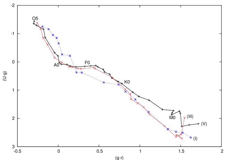
Figure 4: Simulated colours of main sequence (V,black), giant (III, red) and supergiant (I, blue) stars in the UVEX $(U-g)$ vs $(g-r)$ plane.

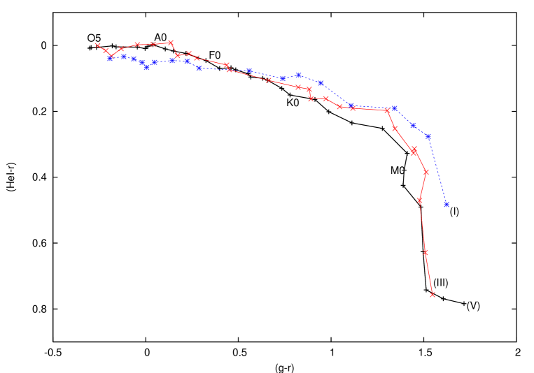
Figure 5: Simulated colours of main sequence (V, black), giant (III, red) and supergiant (I, blue) stars in the UVEX ($He$i$-$$r$ ) vs $(g-r)$ plane.

The prime motivation to chart the population of interacting binaries and stellar remnants in our Galaxy is that a large and homogeneous sample is needed to answer questions in the fields of binary stellar evolution (e.g. on the physics of the common-envelope phase), the gravitational radiation foreground from compact binaries in our Galaxy for missions such as LISA, and the influence of chemical composition on accretion disk physics. For this last item in particular the comparison between hydrogen-rich systems such as Cataclysmic variables and helium-rich (AM CVn stars; e.g. Roelofs et al., 2006) or even C/O-rich (Ultracompact X-ray Binaries; Nelemans et al. 2004) systems will be important. The currently known populations of these last two classes are limited to less than two dozen systems each, severely limiting a population study (see Roelofs, Nelemans & Groot, 2007).

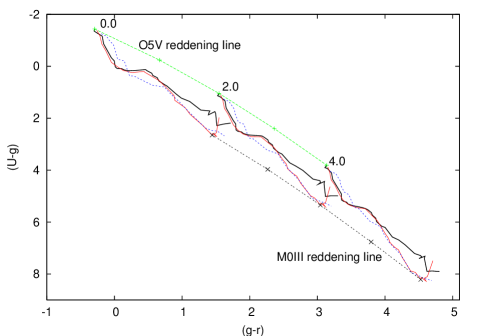
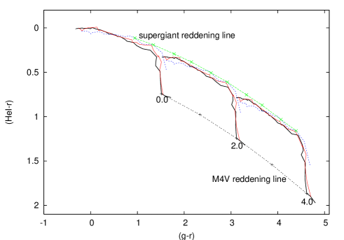
Figure 6: Synthetic colour-colour diagrams in the UVEX filter system for main-sequences, giant and supergiant, using the reddening law of Cardelli et al. (1989). Colours are shown for $E(B-V)=0.0,2.0$ and $4.0$. Also shown are the encompassing upper and lower envelope curves: the O5V reddening curve and the M0iii reddening curve.

Besides the main science goal outlined above, the UVEX survey will allow for many more scientific studies in the field of Galactic astrophysics, especially in combination with the IPHAS survey. The combination of UVEX and IPHAS will allow a much cleaner separation of stellar populations with different intrinsic colours, absolute magnitudes and varying degrees of reddening. The added opportunities include:

• A 3D dust model of our Galaxy on an arcsecond scale: the inclusion of H$\alpha$ with the four broad bands allows for breaking the degeneracy between reddened early type stars and unreddened late type stars due to their strongly different H$\alpha$ absorption lines strength. See Drew et al. (2008) and Sale et al. (2009) for the usage of IPHAS data towards this goal.

• The first ever accurate high proper motion study in the Galactic Plane. The overlap in $r$ band observations between UVEX and IPHAS has a minimum of three years baseline distance, and otherwise identical set-up allows for proper motion determinations down to $\mu\geq$100 mas yr^-1 for the IPHAS - UVEX comparison and down to $\mu\geq$20 mas yr^-1 for an IPHAS - POSS-I comparison; Deacon et al. (2009). These should be compared to the recent surveys by Lépine et al. (see Lépine 2008 and Lépine & Shara, 2005). The combined IPHAS/UVEX proper motions will have more accurate photometry and better completeness, both because CCD observations are used instead of photographic plates.

• The identification and characterisation of open clusters, star forming regions and (highly reddened) O/B associations down to the magnitude limit of the two surveys.

• The characterization of stellar photometric variability on a three-year timescale due to reobservations in the $r$ band. This includes the identification of long period variables (e.g. Mira stars), irregular variables (dwarf novae-type cataclysmic variables, soft X-ray transients, flare stars), and a first identification of large amplitude regular variables (e.g. RR Lyrae stars). EGAPS will also serve as a baseline for new transients in the plane of the Milky Way as shown by our study of Nova Vul 2007 (V458 Vul) whose progenitor was identified in IPHAS data taken only seven weeks before the nova explosion (Wesson et al., 2008).

In the science goals of the UVEX survey the $U$-band observations play a crucial role. Since the $U$-band is the most sensitive to dust extinction it is not only a pivotal band to identify those hot but low-luminosity populations in the Plane, but is also a band that will play a very important role in the dust mapping of the Plane. Straddling the Balmer jump it is also the broad band which is most sensitive to chemical composition and atmospheric pressure in the underlying populations.

3 Survey Design & Data processing

Apart from the filters, the survey design is identical to that of the IPHAS survey as described in D05. The same field centers have been taken so all fields will be imaged twice in a set of overlapping pointings. The order of field selection for UVEX is mainly based on the availability of ‘good’ IPHAS data for the same field with a time baseline of at least three years. Here ‘good’ IPHAS photometry refers to those fields that have a seeing less than 2.0^′′, ellipticity of the stellar image $<$0.2 and a sky background of $<$2000 cts in $r$ (González-Solares et al., 2008). This strategy has been chosen to ensure both a reasonable proper motion baseline as well as a high quality dataset covering the full optical spectrum. UVEX observations are done in the RGO $U$ filter, the Sloan Gunn $g$ and $r$ filters and the $He$i$5875$ filter. Integration times are 120 sec ($U$), 30 sec ($g$), 30 sec ($r$) and 120/180 sec ($He$i).

Fig. 2 shows the throughput of the $U,g,r$ and $He$i$5875$ filters, as well as the IPHAS $r$, $i$ and $H\alpha$, overplotted onto the spectrum of Vega. As can be seen in Fig. 2 the $He$i$5875$ filter overlaps with the $r$-band filter, but has a slightly bluer effective wavelength than the $r$-band. For this reason we construct the ($He$i$-$$r$ ) colour, adhering to the usual notation for colours to list the bluer band first. Note that the $r$-band curve is slightly different from that shown in D05, even though it is the same filter. Filter efficiencies were remeasured in July 2006 at the ING Observatory, resulting in the current efficiency curves.

Data processing is also identical to the IPHAS procedure. All data is transported from the telescope to the Cambridge Astronomy Survey Unit, where it is processed according to the pipeline procedure as detailed in Irwin & Lewis (2001), D05 and González-Solares et al.(2008).

All magnitudes are on the Vega system. The $g$ and $r$ band observations are calibrated on a nightly basis by the observation of photometric standards stars from Landolt (1992). Photometric calibration in $U$, $H\alpha$ and $He$i$5875$ is hard-coupled to that of the $g$-band (for $U$), and the $r$-band filter (for $H\alpha$ and $He$i$5875$). The fixed offsets (in Vega magnitudes) are $U=g-2.100$, $H\alpha=r-3.140$ and $He$i = $r-3.575$. These shifts have been determined on the basis of spectrophotometric observations combined with the colour-modeling discussed in Section 4. On a typical good night the zeropoints (in ADU) for $g$ and $r$ are 25.01 and 24.51 respectively, showing the greater depth of the $g$-band observations for a given integration time. Since the $g$- and $r$-band observations are both 30 seconds, the $g$-band gives the deepest observations of the combined IPHAS /UVEX survey. A global photometric calibration of both surveys remains to be done.

For illustrative purposes Fig. 3 shows the magnitude error as a function of magnitude and colour for the UVEX observations of field 6160, where we have taken all data which have been marked as ‘stellar’ (quality flag ‘–1’ as defined in González-Solares et al., 2008) and on CCD 4 of the Wide Field Camera. Fig. 13 shows the colour-magnitude and colour-colour diagrams for the same field.

4 Simulation of the UVEX colour-colour planes

To interpret the UVEX observations, simulations of the colours of stars and the effect of reddening are a very powerful and important tool. In obtaining the simulated colours we follow the procedure as outlined in D05 for the IPHAS survey. In short, model and template spectra are folded with the efficiency curves as shown in Fig. 2 and the CCD response curve, and calibrated on the Vega system using Eq. 1 of D05, where $r$ and $i$ indices should be replaced with the appropriate filter curves. The only difference in this procedure is that we did not rebin all input data to a 5Å resolution (in D05 set by the resolution of the Pickles, 1998, library), but used a fixed 1Å sampling and a linear interpolation where necessary, as well as an extrapolation on the CCD-efficiency curve on the blue-side of the $U$-band since data was not available. A check on the colours obtained has been made by reproducing the colours as given in D05 for the IPHAS filters (using the filter curves as given in D05). The mean difference and standard deviation on the IPHAS colours derived in D05 and here are $\overline{\Delta(r-i)}=0.009$ and $\sigma_{(r-i)}=0.002$ and $\overline{\Delta(r-H\alpha)}=0.006$ and $\sigma_{(r-H\alpha)}=0.002$. Further checks to the procedure were made by inserting Johnson-Cousins filters into the equation and calculating the colours of main-sequence stars, based on the Pickles spectra, and compared with the colours as given in Bessell (1990) for main-sequence and giant stars and with the Stone & Baldwin (1983) southern spectrophotometric standard stars as given by Landolt (1992).

Our conclusion from these comparisons is that the method accurately reproduces the colours of stars as given in the literature, although there is a large scatter on the $(U-B)$ colours. The relatively large scatter with respect to the stars given in Bessell (1990) can also be attributed to the use of a different set of input spectra (the Vilnius spectra used by Bessell vs. the Pickles spectra used by us). The comparison with the Baldwin-Stone spectrophotometric standards as given by Landolt (1992) and the colours from D05 show the accuracy of the method. All synthetic colours calculated in this paper are given in the Appendices. The large scatter in the U-band is not surprising given its sensitivity to metallicity, atmospheric absorption, and the strong variations in detector reponses that occur at the bluest wavelengths. This procedure was then used to derive the colours in the UVEX filters, for normal stars (luminosity classes V, III and I), emission line objects and white dwarfs.

Based on the colour-simulations presented below, and also folding the Pickles spectra with standard Johnson-Cousins filter curves we derive the following colour-transformations from Johnson-Cousins to the IPHAS /UVEX colour space:

$$(U-g)=1.035\,(U-B)+0.470\,(B-V)-0.017$$ (1)

$$(g-r)=1.044\,(B-V)-0.116\,(V-R)+0.025$$ (2)

$$(r-i)=1.484\,(R-I)-0.389\,(V-R)-0.014$$ (3)

These transformations are valid over the colour-region of $-1.43<(U-g)<2.19$, $-0.30<(g-r)<1.72$ and $-0.17<(r-i)<2.58$. Please note that all magnitudes here are on the Vega system. Transferring to the AB system can be done by using the relations given on the Astronomy Survey Unit’s webpage.

Figure 7: Position of Hei$5875$ emission line objects in the $(g-r)$ vs. ($He$i$-$$r$ ) colour space. Horizontal lines mark objects of equal equivalent widths (EW) in units of Å, vertical lines mark lines of constant reddening, assuming an underlying A0V spectrum.

4.1 UVEX colours of main sequence, giant and supergiant stars

To simulate the colours of normal stars with luminosity classes V (main-sequence dwarfs), III (giants) and I (supergiants) we make use of the Pickles (1998) library. After application of the procedure outlined above, the results are shown in Figs.  4 & 5 and are tabulated in Appendix  A. Here we use the $(g-r)$ vs. $(U-g)$ and the $(g-r)$ vs. ($He$i$-$$r$ ) colour-colour diagrams as our fundamental planes. It can be seen that the difference in colours between main-sequence stars, giants and supergiants is relatively small and all objects are restricted to a narrow band. In the ($g-r$) vs. ($He$i$-$$r$ ) plane a characteristic ‘hook’ is displayed, appearing around M0, after which the stars show a distinct increase in the ($He$i$-$$r$ ) colour, caused by the appearance of strong TiO absorption bands depressing the flux in the Hei band.

To simulate the effect of reddening we have applied the extinction laws of Cardelli, Clayton & Mathis (1989), with a fixed $R$=3.1. Results are shown in Fig. 6. Template and model spectra were first multiplied by the extinction laws and then folded through the filter curves. It is clear from Fig. 6 that, in analogy to the IPHAS colours, also here envelope lines exist, indicating a limit above/underneath which no normal main-sequence stars, giants or supergiants are expected. In Fig. 6 these are indicated with ‘O5V-reddening’ line and ‘M0III reddening line’.

Figure 8: Spectrum of the AM CVn star V396 Hya (Ruiz et al., 2001), overplotted with the UVEX /IPHAS narrow-band filter curves of $He$i$5875$ and $H\alpha$ and the broad-band $g$ and $r$ bands.

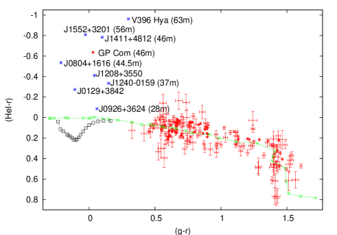
Figure 9: Position of AM CVn stars in a ($g-r$) vs. ($He$i$-$$r$ ) colour-colour diagram. Asterisks show the position of known AM CVn stars, based on their SDSS spectrum. Labels refer to the AM CVn stars and, if known, the orbital period is added (see Roelofs et al., 2009 for SDSS J0804). The AM CVn points are overlayed onto the UVEX colours of stars in the field of GP Com (red symbols), which itself is shown by the (red) point at $(g-r)=0.05$ & $(\hbox{$He${\sc i}$-$$r$\,})=-0.65$. Also shown is the unreddened main-sequence as the green dashed line marked by crosses, and the DB sequence as the purple dotted line marked with squares.

4.2 Colours of helium emission-line stars

The inclusion of the $He$i$5875$ filter has been made to enable the detection of strong $He$i$5875$ absorbers (e.g. DB type white dwarfs) or emitters (e.g. AM Canum Venaticorum stars and Cataclysmic Variables). Again, in analogy with D05 we have determined the sensitivity to pick out Hei emission using an A0V underlying continuum (very similar to a power law slope with index –3) to which an emission line is added. The emission line is simulated by a top-hat shaped line having a width that is equal to the full-width-at-half-maximum of the Hei filter, 40Å. The results are shown in Fig. 7. Reddening has been added to these data in discrete steps of 1 from $E(B-V)=0$ to $E(B-V)=4$. Overplotted onto the grid of emission line strength is the unreddened main-sequence as determined in Sect. 4.1. It can be seen from Fig 7 that emission strength above already a few Å should stand out in UVEX observations, depending mostly on the photometric accuracy of the observations. This is only marginally influenced by reddening due to the narrowness of the Hei filter and its position within the $r$-band. A similar behaviour is seen in the $(r-H\alpha$) colour although the effect is larger there (D05).

4.3 The colours of AM Canum Venaticorum stars

AM Canum Venaticorum (AM CVn) stars are hydrogen-depleted, short-period interacting binaries consisting of a white dwarf primary and a white dwarf or semi-degenerate helium star secondary, sometimes also called ‘Helium Cataclysmic Variables’ (see e.g. Nelemans, 2005, for an overview). These systems show orbital periods in the range 5.4 min $<P_{\rm orb}<65$ min. At longer orbital periods ($P_{\rm orb}\mathrel{\hbox{\hbox to0.0pt{\lower 2.36806pt\hbox{$\sim$}\hss} \kern-3.00003pt\raise 1.72218pt\hbox{$>$}}}30$ min) their spectra are dominated by strong helium emission lines (see e.g. Marsh, 1991; Roelofs et al. 2005,2006a,b). The strongest of these lines is the Hei5875 line. Fig. 8 shows the spectrum of V396 Hya (Ruiz et al., 2001) with the UVEX /IPHAS narrow-band filters of $He$i$5875$ and H$\alpha$ overplotted. It can be seen that the $He$i$5875$ filter width exactly matches the width of the emission line and therefore provides maximum sensitivity to these systems.

Using the publicly available Sloan spectra and the Very Large Telescope spectra as presented in Roelofs et al. (2005, 2006, 2007a,b,c) we constructed a $(g-r)$ vs. ($He$i$-$$r$ ) colour-colour diagram of long period AM CVn stars (Fig. 9). It can be seen that indeed the long period AM CVn stars lie significantly above the main-sequence in ($He$i$-$$r$ ) due to their Hei 5875 emission. The vertical spread of the AM CVn systems indicates increasing Hei equivalent widths at almost constant broad-band colours.

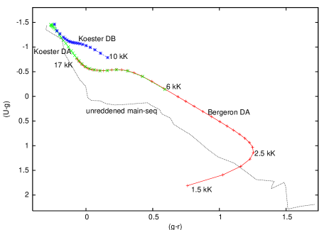
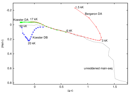
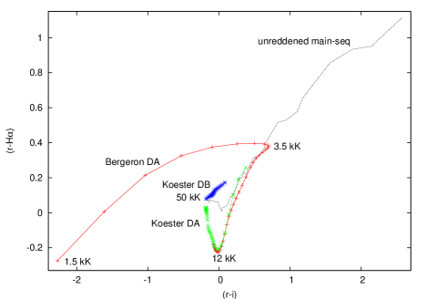
Figure 10: Top: Position of $\log g$=8.0 DA and DB white dwarf in the UVEX $(g-r)$ vs $(U-g)$ colour-colour plane based on the Bergeron models (DA) and Koester models (DA &DB) for temperature between 1 500 K and 80 000 K (DA) and 10 000 - 50 000 K (DB). DB models with temperature $<$10,000 K are identical to blackbodies. The characteristic ‘hook’ in the DA models between temperature 7 000 - 25 000 K is due to the Balmer jump which lies in the U-band. The hook at $T\mathrel{\hbox{\hbox to0.0pt{\lower 2.36806pt\hbox{$\sim$}\hss} \kern-3.00003pt\raise 1.72218pt\hbox{$<$}}}2\,500$K is due to collisionally induced absorption by the H₂ molecule. Middle: Same models as in the previous panel in the ($g-r$) vs.($He$i$-$$r$ ) colour plane. The DA models with $T>3\,000$ K virtually overlay the main-sequence models shown in Fig. 5. The DB models show a pronounced reddening of the $He$i$-$$r$ colour due to the He absorption line at Hei 5875. Bottom: Same models as in the previous panels in the ($r-i$) vs. ($r-H\alpha$) colour, to show the distinction that can be made in these colours between DA and non-DA white dwarfs based on the deep H$\alpha$ absorption.

4.4 Simulation of DA and DB white dwarfs

As uncovering the population of single and binary white dwarfs at low galactic latitude is one of the main goals of the UVEX survey we have also simulated the expected colours of a set of white dwarfs. These simulations are based on two sets of white dwarf model spectra available to us: one set kindly provided by D. Koester, spanning the temperature range 6 000-80 000 K and surface gravity range $\log g$ = 7.0 - 9.0, for both hydrogen dominated atmospheres (DA white dwarfs) as well as helium dominated atmospheres (DB white dwarfs) and one set kindly provided by P. Bergeron spanning the temperature range 1 500 K - 17 000 K and surface gravity range $\log g$ = 7.0 - 9.0, for hydrogen dominated atmospheres (DA white dwarfs). In the coolest models (T $<$ 4 000 K) the effect of collisional induced absorption due to the formation of H₂ was included. See Finley, Koester & Basri (1997), Koester et al. (2001) and Bergeron, Wesemael & Beauchamp (1995) for details on the calculation of these models. Both sets of models were provided on a non-linear wavelength grid, where the lines were more densely sampled than the continuum region. Both sets of models were interpolated on a regular grid with a 1Å binning, identical to the sampling of the filter curves and CCD efficiency. In the overlapping region both sets of models were compared with each other, and were found to be identical on the level of $<2\%$ at all wavelengths with the exception of the very cores of the lines, where differences can increase to $\sim$4% over a small wavelength range.

For the calculation of the white dwarf models we have used the models with a fixed surface gravity of $\log g$ = 8.0. Fig. 10 shows the colours of the white dwarf models in the UVEX colour-colour planes.

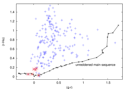
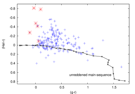
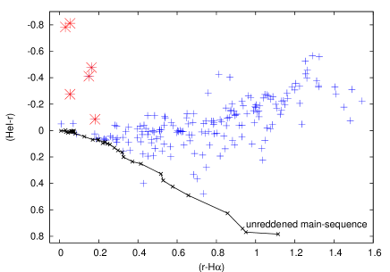
Figure 11: UVEX /IPHAS colour-colour diagram of all currently known Sloan Cataclysmic Variables (‘+’-signs) and AM CVn stars (‘*’-signs) in $(g-r)$ vs. ($R-H\alpha$) (top), $(g-r)$ vs. $He$i$-$$r$ (middle) and ($r-H\alpha$) vs.($He$i$-$$r$ ) (bottom), together with the unreddened main-sequence track.

4.5 Simulations of Cataclysmic Variables

The location of Cataclysmic Variables in H$\alpha$ narrow-band surveys has been extensively discussed in Witham et al., 2006. In IPHAS , based on solely the $r-H\alpha$ and $r-i$ colour, it is difficult to make a photometric distinction between highly reddened background early-type emission line objects and Cataclysmic Variables. With the addition of the UVEX colours this will become easier. Cataclysmic Variables are intrinsically rather faint ($M_{V}\mathrel{\hbox{\hbox to0.0pt{\lower 2.36806pt\hbox{$\sim$}\hss} \kern-3.00003pt\raise 1.72218pt\hbox{$>$}}}$5) but blue, making them on average much less reddened than intrinsically brighter objects at the same colour. We have simulated the position of Cataclysmic Variables in the UVEX survey by taking the sample of Sloan Digital Sky Survey Cataclysmic Variables (Szkody et al. 2002,2003,2004,2005,2006,2007) and folded them through the UVEX filter curves. The $U$-band magnitude could not be calculated due to the blue cut-off in the Sloan Spectra at $\lambda\sim$ 3800 Å. In Fig. 11 we show the colour of all SDSS Cataclysmic Variables and AM CVn stars in the UVEX /IPHAS colour planes.

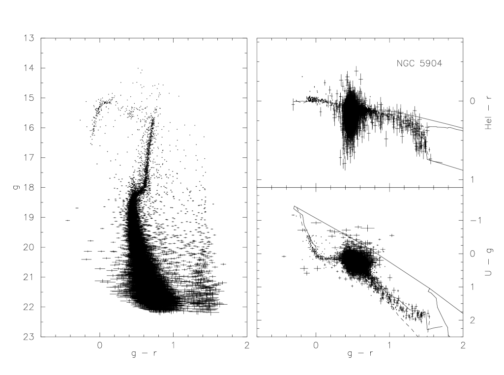
Figure 12: Colour-colour and colour-magnitude diagrams of globular cluster NGC5904 (M5), showing all detected objects with a magnitude error $<0.1$ for clarity, overlayed in the colour-colour diagrams with the UVEX colour-tracks as presented in Sect. 4. Full lines are for main-sequence stars and dashed-lines for giants. The O5-reddening line and the supergiant reddening lines are also shown as the upper and lower envelopes (see Fig. 6 )

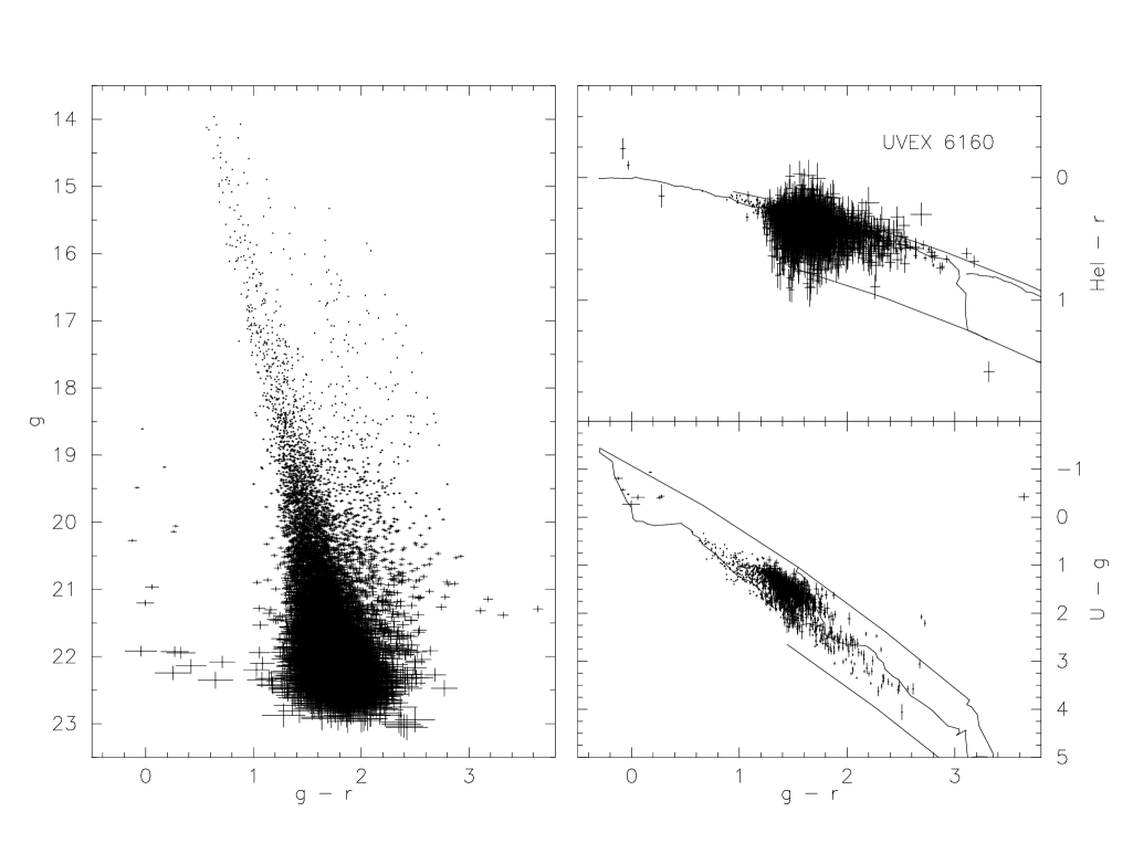
Figure 13: Colour-colour and colour-magnitude diagrams of field 6160, showing all detected objects with a magnitude error $<0.1$ for clarity, overlayed in the colour-colour diagrams with the UVEX colour-tracks as presented in Sect. 4

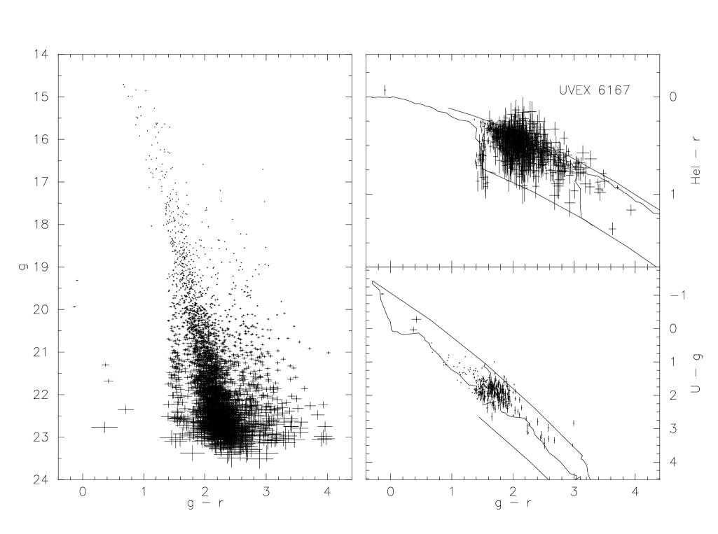
Figure 14: Colour-colour and colour-magnitude diagrams of field 6167, showing all detected objects with a magnitude error $<0.1$ for clarity, overlayed in the colour-colour diagrams with the UVEX colour-tracks as presented in Sect. 4

5 Comparison with observed data

Data taking for UVEX has started in the summer of 2006, and up to September 2008 30% has been observed. After quality control checks all data will be made public through the website of the European Galactic Plane Surveys (EGAPS).

5.1 Control fields & Survey depth

To check our photometric calibration and extraction algorithms in highly crowded areas a number of globular clusters were observed as control fields. In Fig. 12 we show the colour-magnitude and colour-colour diagrams for NGC 5904, overlaid with our main-sequence colour tracks. It is clear from Fig. 12 that the extraction mechanism works very well, even in severely crowded regions. The limiting magnitude (defined here as the magnitude where the magnitude error reaches 0.2 magnitudes (i.e. $\sim 5\sigma$, which would be an error of 0.22 magnitudes) of UVEX data under good conditions ($r$-band seeing of 1$.\!\!^{\prime\prime}$1) is 21.8 ($U$), 22.6 ($g$), 22.1 ($r$) and 20.2 ($He$i$5875$). A limiting magnitude set at 0.2 magnitudes error in the magnitude value encompasses between 95% and 98% of all stellar objects, depending on the filter. Part of the $He$i$5875$ observations are taken with 180 second integration, increasing the limiting magnitude. In general, of course, the limiting magnitude of each individual exposure will depend on seeing, transparency, sky brightness and, in severe cases, also crowding (see Sect. 6).

5.2 Galactic Plane data

In Figs. 13 & 14 we show two representative fields from the Galactic plane centered on ($l,b$=79.6^∘,–2.8^∘) and ($l,b$ =83.0^∘,–0.1^∘), respectively. In the extraction only sources with quality flag ‘–1’ (stellar) and ‘–2’ (probably stellar) have been taken into account and the condition was set that the sources were detected in both the direct as well as the offset fields. In the colour-colour diagrams we overplot the colour-tracks for unreddened data as well as for $E(B-V)$=2.0 and 4.0.

In field 6160 (Fig. 13, $l=79.6$^∘, $b=-2.8$^∘) it can be clearly seen that the main-sequence stars are reddened ($E(B-V)=1.25$ according to Schlegel, Finkbeiner& Davis, 1998). On the blue side a small number of blue excess sources are present, varying in magnitude between $18.5<g<22.5$ and at $g-r\sim 0$. These are unreddened, intrinsically blue and intrinsically low-luminosity objects that lie in front of the bulk of the main sequence population. These are the ‘UV-excess’ sources that give their name to the survey: predominantly white dwarfs and white dwarf binaries. The reddening of the main-sequence causes the bulk of the stars to shift to redder colours overall, uncovering a population of ‘warm’ ($T<$ 10 000 K) white dwarfs. In unreddened (higher galactic latitude) fields these ‘warm’ white dwarfs merge with the main-sequence and become difficult to identify in broad-band photometry. Due to the shallower depth of the $He$i observations the faintest UV-excess sources in $g$ are not detected in the $He$i filter (Fig. 13). Due to their blue colour most are detected in the $U$-band. A distinction between DA and DB white dwarfs can already be made on the basis of the $(U-g)$ vs. $(g-r)$ diagram, but will be further aided by the ($He$i$-r$) vs. $(g-r)$ and the ($He$i$-$$r$ ) vs. ($r-H\alpha$) diagrams.

In field 6167 (Fig. 14) the reddening is higher ($E(B-V)$=3.10 according to Schlegel, Finkbeiner & Davis, 1998), which is not surprising given its location in the mid-plane. The reddening is such that all stars earlier than M0 are substiantially reddened. In the ($He$i$-$$r$ ) vs. $(g-r)$ diagram M-type stars show a distinctive down-turn in the $He$i$-$$r$ colour, making them easily identifiable. The same stars can be seen as the almost vertical sequence at $g-r$=1.5 and running from $19<g<23$. Counter-intuitively the intrinsically faint late-type M-stars have become some of the bluest objects in the field, apart from the real stellar remnants located bluewards of $g-r<$1 and $g>19$.

6 Seeing statistics & Crowding

For all data up to November 2007 we have collected the seeing statistics in the four UVEX filters (Fig. 15). This is for a total of $\sim$375 square degrees and $\sim$3 000 pointings over the period June 2006 - November 2007. It can be seen from Fig. 15 that the median seeing in the UVEX data so far is (1$.\!\!^{\prime\prime}$3,1$.\!\!^{\prime\prime}$1,1$.\!\!^{\prime\prime}$0,1$.\!\!^{\prime\prime}$4) for the ($U,g,r,He$i) filters, respectively. The $He$i data shows a qualitatively different behaviour than the other three bands with a much broader maximum. This is most likely caused by the fact that most of the $He$i data is taken with an integration time of 180 seconds, but with no autoguider. This causes small errors in the telescope tracking, which translate into a deteriorated seeing.

With the stellar densities expected and detected in the Galactic Plane down to g$\sim$22 crowding becomes a real concern for number statistics studies. Surface densities of detected point sources in the UVEX fields can reach up to 200 000 sources per pointing, i.e. 700 000 stars per square degree. Following Irwin & Trimble (1984) we here make a global estimate of the effect of crowding in the UVEX data. Using their Eq. 4 and inserting the relevant numbers for UVEX we calculate the crowding correction factor (i.e. their $f^{\prime}/f$) for seeing disk FWHM values of 0$.\!\!^{\prime\prime}$7 - 1$.\!\!^{\prime\prime}$2 as shown in Fig. 16. As can be seen the crowding factor is a strong function of the actual seeing, and also of the assumed radius of the actual stellar profile. Fig. 16 shows the correction factors for both a 2$\sigma$ Gaussian profile cut-off radius as well as a 3$\sigma$ cut-off. We see that at the maximum density of detected sources in UVEX, which is close to 1 million sources per square degree, we reach a crowding correction of at least 20% in the best of cases (0$.\!\!^{\prime\prime}$7 seeing, 2$\sigma$ cut-off) and quickly reach $>$100% when a 3$\sigma$ cut-off radius is taken. Of course in reality the actual crowding will also depend on the actual magnitude difference between two nearby, almost overlapping sources and will require a detailed field-to-field modeling, but this global estimate shows that for the most crowded regions of the Galactic Plane crowding is a serious issue.

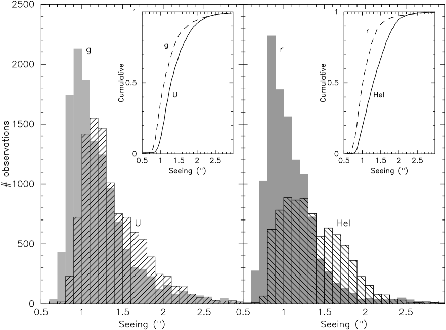
Figure 15: Seeing distributions for UVEX observations in the period June 2006 - November 2007, for the $U$- and $g$-band observations (left panel) and the $r$- and $He$i-band observations (right panel). Inserts show the cumulative distributions.

Figure 16: The crowding correction factor ($f^{\prime}/f$ in the Eq. 4 of Irwin & Trimble, 1984) between observed versus actual number densities of stars for a range in seeing fwhm’s (0.7, 0.8…1.2: lines from bottom to top resp.) and for two settings of the stellar image threshold radius at 2$\sigma$ (dashed lines) and 3$\sigma$ (full lines) Gaussian e-folding lengths.

7 Conclusions

The UVEX survey offers the possibility to detect intrinsically blue, faint objects in the Galactic Plane, as well as offers the first-ever homogeneous blue survey of the Galactic Plane and is ideal for uncovering a large population of stellar remnants. The depth of the $g$-band observations, close to the ground-based confusion limit, will allow for detailed Galactic structure research. The combination with the IPHAS survey offers the first ever optical survey of the Northern Galactic Plane in the $U,g,r,i$, $H\alpha$ and $He$i $5875$ filters. The Southern Plane will be covered by the VPHAS+ survey in the same bands (minus the $He$i band), on the VLT Survey Telescope at the European Southern Observatory. Combined, these three surveys form the heart of the European Galactic Plane Surveys (EGAPS). When completed EGAPS will provide positions, colours for close to one billion stars in our Galaxy. From the first study on proper motions from EGAPS Deacon et al. (2009) showed that we can expect $\sim$140 objects per square degree with a proper motion $\mu\geq$ 20 mas yr^-1.

Appendix A UVEX colours for Main-sequence stars, including reddening

Table 1: UVEX colour indices $(U-g)$, $(g-r)$, $(HeI-r)$ for Pickles main-sequence stars including reddening.

Spec.	$E(B-V)=0.0$			$E(B-V)=1.0$			$E(B-V)=2.0$			$E(B-V)=3.0$			$E(B-V)=4.0$
type	$U$$-$$g$	$g$$-$$r$	$He$i$-$$r$	$U$$-$$g$	$g$$-$$r$	$He$i$-$$r$	$U$$-$$g$	$g$$-$$r$	$He$i$-$$r$	$U$$-$$g$	$g$$-$$r$	$He$i$-$$r$	$U$$-$$g$	$g$$-$$r$	$He$i$-$$r$
O5V	–1.434	–0.294	0.006	–0.239	0.667	0.149	1.044	1.547	0.326	2.400	2.364	0.538	3.811	3.137	0.784
O9V	–1.355	–0.301	0.008	–0.153	0.652	0.151	1.134	1.525	0.329	2.492	2.338	0.541	3.903	3.111	0.788
B0V	–1.293	–0.265	0.006	–0.099	0.691	0.148	1.183	1.567	0.326	2.537	2.381	0.538	3.945	3.152	0.784
B1V	–1.158	–0.180	0.001	0.047	0.767	0.146	1.337	1.635	0.326	2.699	2.442	0.541	4.111	3.209	0.788
B3V	–0.863	–0.160	0.004	0.331	0.785	0.151	1.609	1.651	0.332	2.956	2.458	0.548	4.354	3.226	0.798
B8V	–0.327	–0.045	0.005	0.842	0.895	0.153	2.095	1.757	0.337	3.418	2.561	0.555	4.792	3.326	0.806
B9V	–0.210	–0.003	0.009	0.961	0.932	0.160	2.217	1.791	0.345	3.542	2.592	0.564	4.918	3.355	0.816
A0V	0.026	0.013	0.002	1.196	0.943	0.153	2.451	1.798	0.338	3.775	2.596	0.558	5.149	3.357	0.811
A2V	0.085	0.039	–0.002	1.253	0.969	0.149	2.504	1.823	0.336	3.824	2.621	0.557	5.194	3.383	0.812
A3V	0.090	0.106	0.011	1.267	1.029	0.164	2.528	1.878	0.352	3.856	2.672	0.575	5.233	3.431	0.831
A5V	0.148	0.150	0.017	1.329	1.066	0.171	2.594	1.909	0.361	3.926	2.698	0.585	5.305	3.454	0.842
A7V	0.175	0.217	0.024	1.367	1.134	0.182	2.641	1.978	0.374	3.981	2.769	0.600	5.368	3.526	0.859
F0V	0.158	0.325	0.046	1.370	1.235	0.208	2.662	2.074	0.405	4.017	2.862	0.637	5.416	3.618	0.901
F2V	0.140	0.399	0.070	1.365	1.299	0.235	2.669	2.131	0.435	4.035	2.914	0.669	5.444	3.667	0.935
F5V	0.130	0.460	0.068	1.369	1.355	0.234	2.685	2.182	0.436	4.062	2.962	0.670	5.482	3.713	0.937
F6V	0.177	0.486	0.074	1.416	1.382	0.242	2.732	2.212	0.445	4.109	2.994	0.682	5.529	3.747	0.951
F8V	0.269	0.552	0.086	1.514	1.443	0.256	2.836	2.268	0.462	4.217	3.047	0.701	5.640	3.798	0.971
G0V	0.355	0.567	0.096	1.602	1.455	0.268	2.925	2.280	0.474	4.307	3.060	0.714	5.731	3.811	0.985
G2V	0.438	0.631	0.100	1.695	1.514	0.273	3.028	2.335	0.481	4.417	3.112	0.722	5.847	3.862	0.995
G5V	0.569	0.658	0.106	1.829	1.536	0.280	3.162	2.353	0.489	4.552	3.127	0.732	5.983	3.875	1.005
G8V	0.695	0.734	0.130	1.972	1.610	0.307	3.319	2.427	0.519	4.721	3.202	0.764	6.162	3.951	1.040
K0V	0.769	0.779	0.150	2.036	1.656	0.331	3.376	2.474	0.545	4.771	3.250	0.793	6.204	4.000	1.071
K2V	1.072	0.913	0.164	2.360	1.780	0.346	3.717	2.591	0.563	5.126	3.361	0.813	6.572	4.107	1.093
K3V	1.225	0.988	0.201	2.498	1.864	0.387	3.844	2.681	0.607	5.246	3.454	0.859	6.688	4.201	1.143
K4V	1.356	1.113	0.235	2.648	1.976	0.425	4.009	2.784	0.649	5.424	3.553	0.906	6.877	4.297	1.193
K5V	1.686	1.277	0.252	2.983	2.133	0.443	4.346	2.935	0.667	5.760	3.698	0.923	7.210	4.436	1.209
K7V	1.721	1.411	0.328	3.032	2.250	0.526	4.407	3.038	0.758	5.831	3.791	1.021	7.288	4.522	1.313
M0V	1.806	1.394	0.378	3.109	2.245	0.580	4.478	3.044	0.816	5.895	3.806	1.083	7.347	4.545	1.379
M1V	1.872	1.389	0.425	3.174	2.227	0.628	4.541	3.015	0.865	5.956	3.768	1.133	7.404	4.501	1.430
M2V	1.745	1.485	0.491	3.059	2.320	0.702	4.436	3.105	0.946	5.859	3.857	1.220	7.313	4.590	1.523
M3V	1.821	1.496	0.626	3.143	2.320	0.848	4.525	3.098	1.102	5.949	3.848	1.386	7.401	4.581	1.697
M4V	2.285	1.513	0.742	3.622	2.336	0.977	5.013	3.119	1.244	6.442	3.876	1.542	7.895	4.619	1.866
M5V	2.230	1.605	0.769	3.583	2.423	1.006	4.986	3.202	1.275	6.423	3.956	1.573	7.883	4.696	1.896
M6V	2.189	1.717	0.784	3.568	2.526	1.038	4.988	3.302	1.323	6.437	4.059	1.635	7.904	4.803	1.972

Table 2: UVEX colour indices $(U-g)$, $(g-r)$, $(HeI-r)$ for Pickles Giants including reddening.

Spec.	$E(B-V)$=0.0			$E(B-V)$=1.0			$E(B-V)$=2.0			$E(B-V)$=3.0			$E(B-V)$=4.0
type	$U$$-$$g$	$g$$-$$r$	$He$i$-$$r$	$U$$-$$g$	$g$$-$$r$	$He$i$-$$r$	$U$$-$$g$	$g$$-$$r$	$He$i$-$$r$	$U$$-$$g$	$g$$-$$r$	$He$i$-$$r$	$U$$-$$g$	$g$$-$$r$	$He$i$-$$r$
O8III	–1.382	–0.259	0.001	-0.181	0.696	0.143	1.107	1.571	0.320	2.468	2.383	0.532	3.881	3.154	0.777
B1-2III	–1.170	–0.215	0.016	0.029	0.733	0.160	1.315	1.603	0.340	2.671	2.412	0.554	4.078	3.181	0.801
B3III	–0.852	–0.185	0.032	0.344	0.759	0.179	1.626	1.627	0.361	2.976	2.435	0.578	4.378	3.204	0.828
B5III	–0.619	–0.132	0.010	0.568	0.812	0.158	1.838	1.679	0.341	3.178	2.487	0.559	4.568	3.256	0.810
B9III	–0.148	–0.045	-0.002	1.012	0.895	0.147	2.256	1.757	0.330	3.571	2.561	0.548	4.938	3.326	0.799
A0III	0.013	0.040	–0.003	1.188	0.968	0.147	2.447	1.821	0.333	3.774	2.618	0.552	5.151	3.377	0.805
A3III	0.173	0.136	–0.008	1.348	1.054	0.145	2.605	1.899	0.334	3.930	2.689	0.556	5.304	3.445	0.812
A5III	0.185	0.172	0.031	1.370	1.088	0.186	2.638	1.932	0.377	3.972	2.722	0.603	5.353	3.480	0.861
A7III	0.230	0.234	0.025	1.418	1.150	0.183	2.688	1.994	0.376	4.024	2.784	0.602	5.408	3.541	0.862
F0III	0.241	0.276	0.038	1.435	1.186	0.198	2.711	2.026	0.393	4.051	2.815	0.622	5.439	3.571	0.883
F2III	0.198	0.437	0.060	1.417	1.337	0.226	2.717	2.169	0.427	4.079	2.952	0.662	5.486	3.704	0.929
F5III	0.233	0.451	0.074	1.456	1.352	0.242	2.758	2.186	0.444	4.122	2.971	0.680	5.530	3.726	0.948
G0III	0.555	0.663	0.106	1.812	1.544	0.281	3.144	2.364	0.490	4.533	3.140	0.732	5.961	3.888	1.006
G5III	0.969	0.822	0.127	2.256	1.686	0.307	3.612	2.493	0.522	5.019	3.261	0.770	6.462	4.007	1.048
G8III	1.134	0.883	0.133	2.419	1.740	0.314	3.772	2.543	0.529	5.176	3.307	0.777	6.616	4.049	1.055
K0III	1.313	0.891	0.162	2.597	1.753	0.346	3.948	2.559	0.564	5.351	3.328	0.815	6.789	4.074	1.096
K1III	1.462	0.972	0.162	2.754	1.826	0.346	4.111	2.628	0.565	5.517	3.393	0.816	6.958	4.137	1.098
K2III	1.600	1.047	0.186	2.885	1.897	0.374	4.235	2.696	0.597	5.635	3.458	0.852	7.071	4.200	1.137
K3III	1.852	1.118	0.191	3.148	1.960	0.380	4.507	2.753	0.603	5.915	3.513	0.859	7.356	4.252	1.145
K4III	2.272	1.303	0.198	3.601	2.123	0.391	4.989	2.900	0.619	6.419	3.647	0.878	7.878	4.377	1.168
K5III	2.388	1.345	0.252	3.700	2.175	0.452	5.072	2.959	0.684	6.489	3.712	0.949	7.936	4.448	1.244
M0III	2.651	1.444	0.327	3.969	2.266	0.532	5.345	3.044	0.770	6.763	3.793	1.041	8.211	4.527	1.341
M1III	2.585	1.449	0.313	3.893	2.272	0.518	5.263	3.050	0.757	6.678	3.800	1.028	8.125	4.533	1.328
M2III	2.710	1.513	0.385	4.030	2.337	0.597	5.408	3.117	0.844	6.828	3.870	1.122	8.276	4.607	1.429
M3III	2.608	1.477	0.470	3.923	2.302	0.688	5.298	3.084	0.939	6.716	3.838	1.221	8.163	4.578	1.532
M4III	2.557	1.507	0.629	3.869	2.335	0.858	5.242	3.120	1.121	6.656	3.880	1.415	8.099	4.625	1.736
M5III	1.975	1.547	0.757	3.272	2.390	0.997	4.636	3.186	1.270	6.047	3.954	1.573	7.488	4.707	1.903

Table 3: UVEX /IPHAS colour indices $(U-g)$, $(g-r)$, $(HeI-r)$ for Pickles Supergiants including reddening.

Spec.	$E(B-V)$=0.0			$E(B-V)$=1.0			$E(B-V)$=2.0			$E(B-V)$=3.0			$E(B-V)$=4.0
type	$U$$-$$g$	$g$$-$$r$	$He$i$-$$r$	$U$$-$$g$	$g$$-$$r$	$He$i$-$$r$	$U$$-$$g$	$g$$-$$r$	$He$i$-$$r$	$U$$-$$g$	$g$$-$$r$	$He$i$-$$r$	$U$$-$$g$	$g$$-$$r$	$He$i$-$$r$
B0I	–1.250	–0.193	0.040	-0.034	0.748	0.186	1.267	1.613	0.368	2.635	2.420	0.585	4.053	3.189	0.834
B1I	–1.159	–0.118	0.034	0.056	0.825	0.186	1.354	1.692	0.374	2.720	2.502	0.596	4.134	3.274	0.851
B3I	–0.951	–0.064	0.041	0.251	0.878	0.190	1.539	1.741	0.374	2.896	2.545	0.593	4.303	3.309	0.845
B5I	–0.852	–0.019	0.052	0.358	0.913	0.206	1.651	1.771	0.395	3.010	2.573	0.619	4.417	3.339	0.875
B8I	–0.659	0.005	0.067	0.543	0.931	0.221	1.828	1.783	0.410	3.179	2.581	0.634	4.578	3.344	0.890
A0I	–0.264	0.047	0.051	0.902	0.977	0.206	2.153	1.832	0.397	3.474	2.632	0.621	4.845	3.397	0.879
A2I	–0.217	0.143	0.046	0.964	1.064	0.202	2.229	1.912	0.394	3.563	2.706	0.620	4.946	3.465	0.878
F0I	0.373	0.224	0.048	1.526	1.141	0.208	2.764	1.986	0.403	4.071	2.780	0.633	5.429	3.541	0.896
F5I	0.378	0.288	0.069	1.543	1.204	0.234	2.793	2.050	0.433	4.111	2.846	0.666	5.480	3.609	0.931
F8I	0.728	0.558	0.077	1.938	1.438	0.244	3.225	2.255	0.446	4.574	3.029	0.681	5.967	3.776	0.948
G0I	0.802	0.740	0.101	2.052	1.610	0.274	3.377	2.420	0.482	4.757	3.190	0.724	6.178	3.934	0.997
G2I	1.052	0.825	0.090	2.320	1.682	0.265	3.658	2.483	0.475	5.049	3.246	0.718	6.477	3.986	0.993
G5I	1.330	0.945	0.114	2.617	1.785	0.293	3.969	2.575	0.507	5.369	3.331	0.754	6.804	4.067	1.032
G8I	1.773	1.108	0.183	3.062	1.948	0.371	4.416	2.738	0.593	5.818	3.496	0.848	7.254	4.234	1.133
K2I	2.377	1.342	0.191	3.703	2.153	0.384	5.085	2.922	0.611	6.508	3.665	0.870	7.960	4.392	1.159
K3I	2.473	1.442	0.243	3.799	2.255	0.442	5.183	3.025	0.675	6.608	3.769	0.939	8.064	4.498	1.234
K4I	2.503	1.524	0.276	3.851	2.329	0.479	5.252	3.095	0.715	6.692	3.837	0.983	8.158	4.565	1.281
M2I	2.676	1.624	0.483	4.002	2.433	0.703	5.383	3.205	0.956	6.804	3.954	1.240	8.254	4.690	1.553

Table 4: UVEX /IPHAS colour indices $(U-g)$, $(g-r)$, $(He$i$-r)$ $(r-H\alpha)$ and $(r-i)$ for log(g)=8.0 Bergeron DA white dwarfs including reddening.

T (K)	E(B–V)=0.0					E(B–V)=1.0					E(B–V)=2.0
	$U$$-$$g$	$g$$-$$r$	$He$i$-$$r$	$r$$-$$H\alpha$	$r$$-$$i$	$U$$-$$g$	$g$$-$$r$	$He$i$-$$r$	$r$$-$$H\alpha$	$r$$-$$i$	$U$$-$$g$	$g$$-$$r$	$He$i$-$$r$	$r$$-$$H\alpha$	$r$$-$$i$
1500	1.809	0.761	–0.232	–0.275	–2.272	3.113	1.469	–0.132	–0.030	–1.598	4.475	2.129	–0.004	0.186	–0.901
1750	1.592	1.025	–0.095	0.007	–1.613	2.895	1.772	0.036	0.220	–0.944	4.258	2.469	0.196	0.404	–0.254
2000	1.419	1.160	0.029	0.215	–1.036	2.719	1.939	0.185	0.403	–0.375	4.082	2.669	0.372	0.561	0.303
2250	1.271	1.229	0.118	0.325	–0.531	2.570	2.034	0.293	0.495	0.124	3.931	2.788	0.499	0.634	0.792
2500	1.141	1.254	0.174	0.375	–0.093	2.437	2.078	0.361	0.534	0.562	3.798	2.849	0.580	0.660	1.227
2750	1.030	1.249	0.203	0.393	0.258	2.324	2.084	0.396	0.545	0.920	3.684	2.867	0.622	0.664	1.590
3000	0.936	1.225	0.214	0.396	0.501	2.228	2.068	0.409	0.546	1.174	3.586	2.858	0.638	0.662	1.853
3250	0.850	1.191	0.214	0.393	0.638	2.140	2.040	0.410	0.542	1.320	3.497	2.834	0.639	0.658	2.007
3500	0.768	1.151	0.209	0.386	0.694	2.056	2.003	0.404	0.536	1.381	3.412	2.800	0.633	0.653	2.073
3750	0.687	1.106	0.201	0.378	0.700	1.972	1.962	0.395	0.529	1.390	3.326	2.762	0.622	0.647	2.085
4000	0.603	1.057	0.191	0.368	0.682	1.885	1.916	0.383	0.522	1.373	3.238	2.718	0.609	0.641	2.070
4250	0.512	1.002	0.180	0.357	0.650	1.791	1.865	0.370	0.513	1.342	3.141	2.670	0.594	0.634	2.039
4500	0.412	0.941	0.168	0.344	0.610	1.688	1.808	0.355	0.502	1.303	3.036	2.615	0.577	0.626	2.001
4750	0.307	0.876	0.155	0.329	0.567	1.580	1.747	0.340	0.490	1.261	2.925	2.558	0.559	0.616	1.959
5000	0.201	0.810	0.143	0.311	0.523	1.470	1.686	0.324	0.474	1.218	2.812	2.499	0.541	0.603	1.917
5250	0.100	0.747	0.130	0.288	0.482	1.365	1.626	0.309	0.453	1.178	2.705	2.443	0.523	0.585	1.877
5500	0.006	0.688	0.118	0.260	0.445	1.268	1.572	0.295	0.428	1.141	2.606	2.391	0.506	0.562	1.842
6000	–0.160	0.584	0.098	0.205	0.381	1.097	1.474	0.270	0.377	1.079	2.430	2.298	0.477	0.516	1.780
6500	–0.303	0.494	0.080	0.157	0.327	0.949	1.390	0.249	0.334	1.026	2.279	2.219	0.452	0.476	1.728
7000	–0.409	0.420	0.066	0.117	0.280	0.839	1.321	0.232	0.297	0.980	2.167	2.152	0.432	0.442	1.684
7500	–0.479	0.360	0.055	0.082	0.240	0.766	1.264	0.217	0.265	0.941	2.092	2.098	0.415	0.412	1.646
8000	–0.520	0.310	0.044	0.048	0.204	0.723	1.216	0.204	0.233	0.906	2.047	2.052	0.400	0.383	1.611
8500	–0.539	0.266	0.034	0.014	0.171	0.702	1.174	0.192	0.202	0.873	2.025	2.010	0.385	0.354	1.579
9000	–0.543	0.228	0.023	–0.022	0.140	0.698	1.136	0.178	0.167	0.843	2.020	1.972	0.369	0.322	1.550
9500	–0.537	0.193	0.011	–0.068	0.110	0.703	1.100	0.164	0.124	0.814	2.025	1.935	0.352	0.282	1.522
10000	–0.528	0.160	–0.000	–0.119	0.083	0.713	1.067	0.150	0.076	0.788	2.035	1.901	0.335	0.236	1.497
10500	–0.521	0.132	–0.011	–0.161	0.057	0.719	1.037	0.137	0.037	0.764	2.041	1.869	0.320	0.199	1.474
11000	–0.522	0.106	–0.019	–0.191	0.035	0.718	1.010	0.127	0.008	0.742	2.040	1.842	0.308	0.173	1.453
11500	–0.529	0.082	–0.026	–0.212	0.016	0.711	0.987	0.119	–0.011	0.724	2.033	1.818	0.298	0.155	1.435
12000	–0.536	0.061	–0.031	–0.224	–0.001	0.704	0.966	0.112	–0.021	0.708	2.026	1.797	0.290	0.146	1.420
12500	–0.543	0.044	–0.034	–0.225	–0.013	0.696	0.949	0.108	–0.022	0.696	2.017	1.781	0.286	0.146	1.408
13000	–0.554	0.027	–0.036	–0.223	–0.024	0.684	0.933	0.105	–0.020	0.685	2.004	1.766	0.282	0.149	1.398
13500	–0.572	0.010	–0.038	–0.221	–0.034	0.664	0.918	0.103	–0.017	0.675	1.983	1.752	0.279	0.153	1.387
14000	–0.597	–0.005	–0.039	–0.217	–0.044	0.639	0.905	0.102	–0.013	0.665	1.957	1.740	0.278	0.157	1.378
14500	–0.624	–0.019	–0.039	–0.212	–0.051	0.609	0.893	0.102	–0.007	0.657	1.926	1.730	0.277	0.163	1.370
15000	–0.653	–0.031	–0.039	–0.206	–0.058	0.579	0.882	0.102	–0.001	0.650	1.895	1.721	0.277	0.169	1.363
15500	–0.683	–0.042	–0.038	–0.199	–0.064	0.548	0.873	0.102	0.006	0.644	1.863	1.713	0.278	0.176	1.356
16000	–0.712	–0.052	–0.038	–0.192	–0.070	0.518	0.865	0.102	0.013	0.638	1.832	1.706	0.278	0.183	1.350
16500	–0.741	–0.061	–0.038	–0.184	–0.075	0.488	0.857	0.103	0.020	0.633	1.801	1.700	0.278	0.190	1.345
17000	–0.769	–0.070	–0.038	–0.177	–0.079	0.460	0.850	0.103	0.027	0.629	1.772	1.695	0.279	0.197	1.340

Table 4: , continued

Table 5: UVEX /IPHAS colour indices $(U-g)$, $(g-r)$, $(HeI-r)$ $(r-H\alpha)$ and $(r-i)$ for log(g)=8.0 Koester DA white dwarfs including reddening

T (K)	E(B–V)=0.0					E(B–V)=1.0					E(B–V)=2.0
	$U$$-$$g$	$g$$-$$r$	$He$i$-$$r$	$r$$-$$H\alpha$	$r$$-$$i$	$U$$-$$g$	$g$$-$$r$	$He$i$-$$r$	$r$$-$$H\alpha$	$r$$-$$i$	$U$$-$$g$	$g$$-$$r$	$He$i$-$$r$	$r$$-$$H\alpha$	$r$$-$$i$
6000	–0.141	0.591	0.102	0.257	0.378	1.115	1.482	0.275	0.429	1.074	2.448	2.306	0.483	0.566	1.775
7000	–0.403	0.423	0.072	0.191	0.275	0.844	1.325	0.238	0.369	0.974	2.171	2.158	0.439	0.513	1.677
8000	–0.517	0.312	0.047	0.101	0.200	0.726	1.219	0.208	0.286	0.901	2.049	2.056	0.404	0.435	1.606
9000	–0.541	0.228	0.024	–0.009	0.139	0.700	1.136	0.179	0.180	0.841	2.022	1.973	0.370	0.335	1.548
10000	–0.524	0.160	0.000	–0.117	0.083	0.717	1.066	0.151	0.078	0.788	2.039	1.900	0.336	0.239	1.497
11000	–0.521	0.105	–0.018	–0.183	0.035	0.720	1.010	0.129	0.017	0.742	2.043	1.841	0.310	0.181	1.453
12000	–0.537	0.063	–0.028	–0.207	0.002	0.703	0.968	0.116	–0.005	0.710	2.024	1.799	0.294	0.162	1.422
13000	–0.561	0.028	–0.033	–0.208	–0.022	0.677	0.935	0.109	–0.005	0.687	1.997	1.768	0.286	0.164	1.400
14000	–0.602	–0.004	–0.037	–0.205	–0.042	0.634	0.905	0.104	–0.001	0.667	1.952	1.741	0.281	0.168	1.379
15000	–0.658	–0.030	–0.037	–0.196	–0.057	0.575	0.883	0.104	0.008	0.651	1.892	1.722	0.279	0.178	1.364
16000	–0.718	–0.051	–0.037	–0.184	–0.069	0.514	0.866	0.104	0.021	0.639	1.828	1.707	0.280	0.191	1.351
17000	–0.775	–0.069	–0.036	–0.170	–0.078	0.454	0.851	0.104	0.034	0.629	1.767	1.695	0.280	0.204	1.341
18000	–0.829	–0.084	–0.036	–0.158	–0.087	0.398	0.838	0.105	0.047	0.621	1.710	1.685	0.280	0.217	1.332
19000	–0.879	–0.098	–0.036	–0.147	–0.094	0.347	0.827	0.105	0.057	0.613	1.658	1.675	0.280	0.227	1.324
20000	–0.924	–0.110	–0.036	–0.138	–0.101	0.301	0.816	0.105	0.067	0.606	1.610	1.666	0.280	0.237	1.317
22000	–1.004	–0.132	–0.036	–0.124	–0.114	0.219	0.798	0.104	0.081	0.593	1.527	1.651	0.279	0.251	1.304
24000	–1.072	–0.151	–0.037	–0.114	–0.125	0.149	0.781	0.103	0.091	0.581	1.456	1.637	0.278	0.262	1.292
26000	–1.132	–0.170	–0.037	–0.106	–0.136	0.087	0.766	0.103	0.100	0.571	1.392	1.623	0.277	0.270	1.281
28000	–1.188	–0.185	–0.037	–0.095	–0.145	0.030	0.752	0.102	0.111	0.561	1.333	1.612	0.277	0.282	1.271
30000	–1.239	–0.198	–0.037	–0.078	–0.152	–0.023	0.742	0.103	0.127	0.553	1.279	1.603	0.277	0.298	1.263
35000	–1.322	–0.219	–0.035	–0.038	–0.163	–0.108	0.725	0.105	0.167	0.542	1.192	1.590	0.279	0.337	1.252
40000	–1.362	–0.231	–0.034	–0.017	–0.169	–0.150	0.716	0.106	0.188	0.536	1.149	1.583	0.280	0.359	1.245
45000	–1.386	–0.239	–0.034	–0.004	–0.172	–0.175	0.709	0.106	0.201	0.532	1.123	1.578	0.281	0.372	1.241
50000	–1.403	–0.244	–0.034	0.005	–0.175	–0.193	0.704	0.106	0.210	0.529	1.104	1.574	0.281	0.381	1.238
55000	–1.416	–0.249	–0.034	0.012	–0.177	–0.206	0.700	0.107	0.217	0.527	1.090	1.570	0.281	0.387	1.236
60000	–1.427	–0.253	–0.033	0.017	–0.179	–0.217	0.697	0.107	0.222	0.525	1.079	1.568	0.281	0.392	1.234
65000	–1.435	–0.256	–0.033	0.021	–0.181	–0.226	0.694	0.107	0.226	0.523	1.070	1.565	0.282	0.397	1.232
70000	–1.443	–0.259	–0.033	0.025	–0.183	–0.234	0.692	0.107	0.230	0.522	1.062	1.563	0.282	0.400	1.230
75000	–1.449	–0.262	–0.033	0.027	–0.184	–0.241	0.690	0.107	0.232	0.520	1.055	1.562	0.281	0.403	1.229
80000	–1.455	–0.264	–0.033	0.030	–0.185	–0.247	0.688	0.107	0.235	0.519	1.049	1.560	0.281	0.405	1.227

Table 5: , continued

Table 6: UVEX /IPHAS colour indices $(U-g)$, $(g-r)$, $(HeI-r)$ $(r-H\alpha)$ and $(r-i)$ for log(g)=8.0 Koester DB white dwarfs including reddening.

T (K)	E(B–V)=0.0					E(B–V)=1.0					E(B–V)=2.0
	$U$$-$$g$	$g$$-$$r$	$He$i$-$$r$	$r$$-$$H\alpha$	$r$$-$$i$	$U$$-$$g$	$g$$-$$r$	$He$i$-$$r$	$r$$-$$H\alpha$	$r$$-$$i$	$U$$-$$g$	$g$$-$$r$	$He$i$-$$r$	$r$$-$$H\alpha$	$r$$-$$i$
10000	–0.787	0.162	0.033	0.172	0.081	0.444	1.083	0.189	0.361	0.781	1.757	1.930	0.380	0.515	1.485
11000	–0.874	0.109	0.031	0.161	0.049	0.353	1.033	0.186	0.351	0.749	1.664	1.883	0.375	0.507	1.453
12000	–0.944	0.067	0.037	0.153	0.023	0.281	0.995	0.190	0.345	0.724	1.590	1.848	0.378	0.502	1.428
13000	–0.993	0.032	0.050	0.146	–0.000	0.231	0.962	0.202	0.339	0.701	1.539	1.816	0.388	0.498	1.406
14000	–1.029	0.001	0.072	0.140	–0.020	0.193	0.933	0.223	0.334	0.681	1.500	1.788	0.408	0.494	1.386
15000	–1.053	–0.024	0.101	0.135	–0.037	0.168	0.908	0.250	0.330	0.665	1.475	1.764	0.435	0.491	1.370
16000	–1.068	–0.045	0.134	0.130	–0.050	0.153	0.888	0.283	0.326	0.652	1.460	1.744	0.466	0.488	1.358
17000	–1.077	–0.063	0.167	0.125	–0.060	0.144	0.870	0.314	0.322	0.643	1.451	1.725	0.497	0.485	1.349
18000	–1.083	–0.078	0.194	0.120	–0.068	0.138	0.855	0.341	0.318	0.635	1.445	1.709	0.522	0.481	1.343
19000	–1.089	–0.091	0.212	0.115	–0.075	0.132	0.841	0.358	0.314	0.629	1.440	1.695	0.539	0.478	1.337
20000	–1.095	–0.103	0.220	0.111	–0.081	0.126	0.830	0.366	0.310	0.624	1.433	1.684	0.546	0.475	1.332
22000	–1.105	–0.117	0.216	0.107	–0.088	0.115	0.816	0.361	0.306	0.617	1.423	1.670	0.541	0.471	1.325
24000	–1.118	–0.128	0.199	0.104	–0.094	0.102	0.807	0.343	0.304	0.611	1.408	1.662	0.523	0.469	1.319
26000	–1.141	–0.142	0.185	0.100	–0.103	0.077	0.793	0.329	0.301	0.602	1.383	1.650	0.508	0.467	1.310
28000	–1.169	–0.156	0.175	0.098	–0.113	0.048	0.781	0.319	0.299	0.592	1.353	1.639	0.497	0.465	1.300
30000	–1.199	–0.169	0.164	0.096	–0.122	0.018	0.770	0.307	0.297	0.583	1.321	1.630	0.485	0.464	1.291
35000	–1.270	–0.196	0.134	0.092	–0.139	–0.056	0.747	0.277	0.294	0.565	1.244	1.611	0.454	0.461	1.274
40000	–1.329	–0.218	0.116	0.088	–0.154	–0.117	0.728	0.258	0.290	0.551	1.182	1.594	0.435	0.459	1.259
50000	–1.463	–0.236	0.038	0.080	–0.180	–0.256	0.717	0.180	0.284	0.524	1.039	1.589	0.355	0.453	1.232

Table 6: , continued

References

- Anderson et al. (2005) Anderson S.F., Haggard D., Homer L., et al., 2005, AJ 130, 2230
- Anderson et al. (2008) Anderson S.F., Haggard D., Homer L., et al., 2008, AJ 135, 2108
- Bergeron (1995) Bergeron P., Wesemael F. & Beauchamp A., 1995, PASP 107, 1047
- Bessell (1990) Bessell M.S., 1990, PASP 102, 1181
- Boissier&Prantzos (1999) Boissier S. & Prantzos N., 1999, MNRAS 307, 857
- Cardelli et al. (1989) Cardelli J.A., Clayton G.C. & Mathis J.S., 1989, ApJ 345, 245
- Deacon et al. (2008) Deacon N., Groot P.J., Irwin M., Drew J., Greimel R., et al., 2009, MNRAS, accepted, arXiv:0905.2594
- Drew et al. (2005) Drew J., Greimel R., Irwin M., et al., 2005, MNRAS 362, 753 (D05)
- Drew et al. (2008) Drew J., et al., 2008, MNRAS 386, 1761
- Finley, Koester & Basri (1997) Finley D.S., Koester D., Basri G., 1997, ApJ 488, 375
- González-Solares et al. (2008) González-Solares E.A., Walton N.A., Greimel R., Drew J.E., et al., 2008, MNRAS 388, 89
- Irwin&Trimble (1984) Irwin M. & Trimble V., 1984, AJ 89, 83
- Irwin&Lewis (2001) Irwin M. & Lewis J., 2001, NewAR 45, 105
- Koester et al. (2001) Koester D., et al., 2001, A&A 378, 556
- Landolt (1992) Landolt A., 1992, AJ 104, 340
- Lanning (1973) Lanning H.H., 1973, PASP 85, 70
- Lanning&Lepine (2006) Lanning H.H. & Lépine S., 2006, PASP 118, 1639
- Lanning&Meakes (2004) Lanning H.H & Meakes M., 2004, PASP 116, 1039
- Lépine (2008) Lépine S., AJ 135, 2177
- Lépine&Shara (2005) Lépine S., & Shara M.M., 2005, AJ 129, 1483
- Marsh et al. (1991) Marsh T.R, Horne K. & Rosen S., 1991, ApJ 366, 535
- Nelemans (2005) Nelemans G., 1995, ASPC 330, 27
- Nelemans et al. (2005) Nelemans G., Jonker P.G., Marsh T.R. & Van der Klis M., 2004, MNRAS 348, L7
- Nelemans et al. (2004) Nelemans G., Yungelson L.R. & Portegies Zwart S.F., 2004, MNRAS 349, 181
- Pickles A.J. (1998) Pickles A.J., 1998, PASP 110, 863
- Roelofs et al. (2005) Roelofs G.H.A., Groot P.J., Marsh T.R., Steeghs D., Barros S.C.C., Nelemans G., 2005, MNRAS 361, 487
- Roelofs et al. (2006a) Roelofs G.H.A., Groot P.J., Marsh T.R., Steeghs D., Nelemans G.,2006, MNRAS 365, 1109
- Roelofs et al. (2006b) Roelofs G.H.A., Groot P.J., Marsh T.R., Steeghs D., Nelemans G.,2006, MNRAS 371, 1231
- Roelofs et al. (2007) Roelofs G.H.A., Nelemans G. & Groot P.J., 2007, MNRAS 382, 685
- Roelofs et al. (2009) Roelofs G.H.A., Groot, P.J., Steeghs, D.H.A, et al., 2009, MNRAS 394, 367
- Ruiz et al. (2001) Ruiz M.T., Rojo P.M., Garay G., Maza J., 2001, ApJ 552, 679
- Sale (2009) Sale S., Drew J., Unruh Y., et al., 2009, MNRAS 392, 497
- Sandage (1972) Sandage A., 1972, ApJ 178, 1
- Schlegel, Finkbeiner& Davis (1998) Schlegel D.J., Finkbeiner D.P. & Davis, M., 1998, ApJ 500, 525
- Steinmetz et al. (2006) Steinmetz M., Zwitter T., Siebert A., et al., 2006, AJ 132, 1645
- Baldwin&Stone (1983) Stone R.P.S & Baldwin J.A., 1983, MNRAS 204, 347
- Szkody et al. (2002) Szkody P., et al., 2002, AJ 123, 430
- Szkody et al. (2003) Szkody P., et al., 2003, AJ 126, 1499
- Szkody et al. (2004) Szkody P., et al., 2004, AJ 128, 1882
- Szkody et al. (2005) Szkody P., et al., 2005, AJ 129, 2386
- Szkody et al. (2006) Szkody P., et al., 2006, AJ 131, 973
- Szkody et al. (2007) Szkody P., et al., 2007, AJ 134, 185
- Wesson et al. (2008) Wesson R., Barlow M., Corradi R., et al., 2008, ApJ 688, L21
- Witham et al. (2006) Witham A.R., et al., 2006, MNRAS 369, 581
- Yanny et al. (2009) Yanny B., Rockosi C., Newberg H.J., et al., 2009, AJ 137, 4377