The Fundamental Plane of Accretion onto Black Holes with Dynamical Masses

Abstract

Black hole accretion and jet production are areas of intensive study in astrophysics. Recent work has found a relation between radio luminosity, X-ray luminosity, and black hole mass. With the assumption that radio and X-ray luminosity are suitable proxies for jet power and accretion power, respectively, a broad fundamental connection between accretion and jet production is implied. In an effort to refine these links and enhance their power, we have explored the above relations exclusively among black holes with direct, dynamical mass-measurements. This approach not only eliminates systematic errors incurred through the use of secondary mass measurements, but also effectively restricts the range of distances considered to a volume-limited sample. Further, we have exclusively used archival data from the Chandra X-ray Observatory to best isolate nuclear sources. We find $\log{L_{R}}=\left(4.80\pm 0.24\right)+\left(0.78\pm 0.27\right)\log{M_{\mathrm{BH}}}+\left(0.67\pm 0.12\right)\log{L_{X}}$, in broad agreement with prior efforts. Owing to the nature of our sample, the plane can be turned into an effective mass predictor. When the full sample is considered, masses are predicted less accurately than with the well-known $M$–$\sigma$ relation. If obscured AGN are excluded, the plane is potentially a better predictor than other scaling measures.

1. Introduction

Accretion onto black holes has many observable consequences, including the production of relativistic jets. The phenomenon of jet production appears to be universal, as such jets are observed both in Active Galactic Nuclei (AGN) and stellar-mass black hole systems as well as in neutron stars, white dwarfs, and even young stellar objects. For black hole sources, the length scales and relevant timescales of jets appear to approximately scale with mass over 8 orders of magnitude, giving rise to the possibility that jet production mechanisms scale with mass, similar to the way that accretion disk properties scale. The mechanism by which jets are driven from black holes, however, remains observationally elusive. It remains one of the most compelling and important problems in astrophysics, particularly in high energy astrophysics. The impact of relativistic jets on the interstellar medium (Gallo et al., 2005b), and large-scale structure in clusters of galaxies (Allen et al., 2006; Fabian et al., 2003; McNamara et al., 2006), has become dramatically clear in the era of imaging and spectroscopy with Chandra.

Virtually all theories of jet production tie the jet to the accretion disk directly or indirectly (see, e.g., Lynden-Bell, 1978; Blandford & Payne, 1982, see also van Putten 2009). Thus, there is a broad expectation that jet properties might depend on the mass accretion rate ($\dot{M}$) through the disk. The black hole spin parameter ($a\equiv cJ/GM^{2}$; $0<a<1$) may also be an important factor if the black hole and accretion disk are linked through magnetic fields (Blandford & Znajek, 1977). The spin is also important for accretion disk jet-launching because the inner radius of the accretion will decrease, thus increasing the launch velocity. This idea may find some support in the dichotomy between radio-loud and radio-quiet AGN (Sikora et al., 2007). The high flux of stellar-mass black holes facilitates spin constraints with current X-ray observatories; in those systems, the most relativistic jets appear to be launched by black holes with high spin parameters (Miller et al., 2009).

One means by which jet production can be examined is to explore correlations between proxies for mass inflow and jet outflow. In stellar-mass black holes, it was found that radio emission and X-ray emission are related by $L_{R}\propto L_{X}^{0.7}$ (Gallo et al., 2003). This correlation was quickly extended to also include super-massive black holes in AGN, resulting in the discovery of a “fundamental plane” of black hole activity (Merloni et al., 2003; Falcke et al., 2004, also see Merloni et al. 2006). The plane can be described by $\log L_{R}=7.33+0.60\log L_{X}+0.78\log M_{\mathrm{BH}}$, with a scatter of $\sigma_{R}=0.88\ \mathrm{dex}$ (where $L_{R}$ is $\nu=5\ \mathrm{GHz}$ nuclear radio luminosity in units of $~{}\mathrm{erg\,s^{-1}}$, $L_{X}$ is $E=2$–$10\ \mathrm{keV}$ nuclear X-ray luminosity in units of $~{}\mathrm{erg\,s^{-1}}$, and $M_{\mathrm{BH}}$ is the black hole’s mass in units of ${\rm M}_{\scriptscriptstyle\odot}$; Merloni et al. 2003; Falcke et al. 2004). Several recent works have revisited the original findings with slightly different focuses. Körding et al. (2006) found that sources emitting far under their Eddington limits followed the relation more tightly. Wang et al. (2006) found differences in the relationship for radio-loud and radio-quiet AGNs. Li et al. (2008) used a large sample of SDSS-identified broad-line AGNs to study a similar relation at lower-frequency (1.4 GHz) radio luminosity and softer-band (0.1–2.4 keV) X-ray luminosities. Yuan et al. (2009) limited the sample to those sources with $L_{X}/L_{\mathrm{Edd}}<10^{-6}$ based on predictions that the correlation between radio and X-ray luminosity steepens to $L_{R}\propto L_{X}^{1.23}$ at low accretion rates (Yuan & Cui, 2005).

It is difficult to overstate the potential importance of the fundamental plane; it suggests that black holes regulate their radiative and mechanical luminosity in the same way at any given accretion rate scaled to Eddington, $\dot{m}=\dot{M}/\dot{M}_{\mathrm{Edd}}$. In the context of models that assume jet properties do scale simply with mass (e.g., Falcke & Biermann, 1995; Heinz & Sunyaev, 2003), the fundamental plane can even be used to constrain the nature of the accretion inflow. At present, radiatively-inefficient inflow models for X-ray emission, and models associating X-ray flux with synchrotron emission near the base of a jet, are both consistent with the fundamental plane.

To use the fundamental plane as a tool and a diagnostic instead of as an empirical correlation, however, it must be sharpened. Black hole masses represent a significant source of uncertainty and scatter in the fundamental plane (Merloni et al., 2003; Körding et al., 2006). In this work, we have constructed a fundamental plane using only black holes with masses that have been dynamically determined, the so-called $M$–$\sigma$ black holes (see Gültekin et al., 2009b). Unlike prior treatments, our X-ray data is taken from a single observatory and predominately from a single observing mode, and we have conducted our own consistent analysis of the data. We analyzed every archival Chandra X-ray observation of black holes with a dynamically-determined mass. Radio data were taken from archival observations reported in the literature. By using a sample of black holes with dynamical masses, we may probe the fundamental plane without subjecting the analysis to the systematic errors inherent in substituting scaling-relation-derived quantities for black hole masses.

In Section 2 we describe the sample of black holes used in this work. We detail our X-ray data reduction and spectral fits in Section 3. Our fitting methods and results are presented in Section 4. We discuss our results in Section 5 and summarize in Section 6.

2. Sample of Black Holes

We get $M_{\mathrm{BH}}$ from the list of black hole masses compiled in Gültekin et al. (2009b), adopting the same distances as well. This sample of black hole masses includes measurements based on high spatial resolution line-of-sight stellar velocity measurements (e.g., Gültekin et al., 2009a), stellar proper motions in our Galaxy (Ghez et al., 2008; Gillessen et al., 2008), gas dynamical measurements (e.g., Barth et al., 2001), and maser measurements (e.g., Miyoshi et al., 1995). It does not include reverberation mapping measurements, which are direct measurements of mass but are secondary in that they are normalized to the other measurements via the $M$–$\sigma$ relation (e.g., Peterson et al., 2004; Onken et al., 2004). From those available black hole masses we use only the measured black hole masses used in their $M$–$\sigma$ fits—not upper limits and not the “omitted sample,” which contains a list of masses with potential problems because (1) masses were listed as tentative by the original study, (2) there was no quantitative analysis of how well the original study’s model fit the data, or (3) the quantitative analysis of the goodness of fit was poor. We reduce available Chandra data and present X-ray luminosities for this collection of potentially problematic masses, but we do not use them in our fits. Thus, we use only the black hole masses with the most reliable measurements.

One of the benefits of using this sample is that most of the distances to the galaxies are less than $30\ ~{}\mathrm{Mpc}$. This distance is close enough that interestingly low X-ray and radio luminosities will still be measurable. So while this is not a true volume-limited sample, it is insensitive to the potential biases arising from, e.g., a sample limited by X-ray flux. Unlike other samples, however, our sample may be biased to very low nuclear luminosities. The contamination from a bright AGN typically causes problems in determining stellar mass-to-light ratio at the center so that most galaxies selected for dynamical measurement do not contain bright AGN. Spiral galaxies, which are less massive on average than early-type galaxies, may also be underrepresented in this sample, and thus low-mass black holes may also be underrepresented.

The radio data we use are 5 GHz peak power measurements from the Ho (2002) compilation of nuclear radio sources. The data were compiled to probe whether there was a correlation between $M_{\mathrm{BH}}$ and $L_{R}$and thus are ideal for our purposes.

3. X-ray Analysis

3.1. X-ray Data Reduction

The high spatial resolution of Chandra enables nuclear emission to be isolated best compared to other X-ray observatories. We used Chandra archival data to obtain accurate measurements or tight upper limits of the flux between 2 and 10 keV for all galaxies in our sample. This energy range was chosen to probe accretion power rather than total power including any contaminating diffuse emission and for ease in comparison to previous fundamental plane work.

For each source we used a circular extraction region positioned at the brightest point source that was consistent with the center of galaxy determined by 2MASS images. There are no nuclear point sources in NGC 1399 and NGC 4261, which we handled slightly differently as described below. For extraction of background spectra, we typically used an annular region with inner radius slightly larger than the source region radius. The outer radius was made large enough to encompass a significant number of counts. Point sources were excluded from the background region. When there were a large number of point sources in the annular region surrounding the source, a different region was used, usually an off-nuclear circle. In these cases we selected a region where the background looked to be similar to that surrounding the source.

Two cases require special attention to contamination from non-nuclear X-ray emission: NGC 0224 (M31) and NGC 4486 (M87). NGC 0224 has two bright point sources near the center of the galaxy, but neither is the galaxy’s central black hole, from which the emission is too dim to be detected above the background to high significance ($L_{X}\mathrel{\hbox to0.0pt{\lower 3.0pt\hbox{$\mathchar 536\relax$}\hss}\raise 2.0pt\hbox{$\mathchar 316\relax$}}10^{36}\,~{}\mathrm{erg\,s^{-1}}$ at at assumed distance of $D=0.8\,~{}\mathrm{Mpc}$ Garcia et al., 2005; Li et al., 2009). NGC 4486 is well known for its prominent jet with several knots. These knots are apparent in the Chandra images. In the high spatial resolution Hubble Space Telescope (HST) images, one knot is very close ($0\farcs 85$ Harris et al., 2006) to the central engine. As the knot has grown brighter in the optical by a factor of $\sim 100$ over the last $\sim 10$ years, measurements of the core X-ray flux become increasingly contaminated by the knot. We chose the archival Chandra data set where the knot was most readily distinguishable from the core.

For the galaxies NGC 1399 and NGC 4261, there is no discernible point source at their nuclei, which are dominated in X-rays by hot gas. For these two sources, we attempt to measure a hypothetical point source at the center. We use a circular region at the center of the diffuse X-ray emission for source extraction with an annular background extraction region immediately adjacent. For both these sources, X-ray point source flux could not be inferred above the background, and they are listed as upper limits in Table The Fundamental Plane of Accretion onto Black Holes with Dynamical Masses.

Data reduction followed the standard pipeline, using the most recent Chandra data reduction software package (CIAO version 4.1.1) and calibration databases (CALDB version 4.1.2). Point-source spectra were extracted using the CIAO tool psextract. Because all observations of interest were done with the Advanced CCD Imaging Spectrometer (ACIS), we ran psextract with the mkacisrmf tool to create the response matrix file (RMF) and with mkarf set for ACIS ancillary response file (ARF) creation.

3.2. X-ray Spectral Fitting

We modeled the reduced spectra using XSPEC12 (Arnaud, 1996). If binning the spectra in energy so that each bin contained a minimum of 20 counts resulted in five or more bins, we did so and used $\chi^{2}$ statistics; otherwise we did not bin the data and used $C$-stat statistics (Cash, 1979). Each spectrum was modeled with a photoabsorbed power-law model. If such a model did not adequately fit the spectrum for data sets that were strong enough to support a more complicated model, we added additional model components. Galaxies that were identified as Seyfert 2 or transitional Seyferts in Véron-Cetty & Véron (2006) were modeled with a partially photoabsorbed power-law, representing intrinsic absorption plus another photoabsorbed component, representing Galactic absorption. Galaxies with obvious diffuse hot gas towards their nucleus were modeled with photoabsorbed Astrophysical Plasma Emission Code (APEC Smith et al., 2001) and power-law components. Regardless of the continuum model, for spectra that showed an obvious Fe K$\alpha$ line, we added a Gaussian for each line. All spectra were fit from $E=0.5$ to $10~{}\mathrm{keV}$.

We considered a model successful if it yielded a reduced $\chi^{2}$ of $\chi^{2}/\nu\leq 2$ and if the spectrum between $E=2$ and $10\ \mathrm{keV}$ was adequately described. The total flux between $E=2$ and $10\ \mathrm{keV}$, $F_{X,\mathrm{tot}}$, was determined from the model and the 1$\sigma$ errors derived from covariance of the model parameters. We then calculated the unabsorbed flux arising from just the power-law component between $E=2$ and $10\ \mathrm{keV}$, $F_{X}$. That is, we de-absorbed the flux and removed contributions from lines and other model components. We assume the fractional error in $F_{X,\mathrm{tot}}$ is the same as in $F_{X}$.

For sources that did not constrain the flux from the central point source, we used the total count rate between $E=0.5$ and $10\mathrm{keV}$ to calculate the 3$\sigma$ (99.7% confidence) upper limit to $F_{X}$ with PIMMS assuming a power-law with index $\Gamma=2$ and with Galactic absorption determined from the Leiden/Argentine/Bonn survey of Galactic HI (Kalberla et al., 2005; Hartmann & Burton, 1997; Bajaja et al., 2005) using the HEASOFT ftool “N_H”.

Because we are ultimately interested in an accurate measurement of $F_{X}$, it is more important that our models characterize the spectrum well over the 2 to 10 keV band than it is to reproduce the underlying physics. We tested this approach by fitting several different models to the same spectrum and recovered consistent values for $F_{X}$. The results of fits are displayed in Table 2, and we show four example spectra with models in Figure 1.

Figure 1.— Example Chandra spectra with best-fit models. The models have been folded through the instrument response. The horizontal error bars show the binning used for the fits. These four galaxies were chosen to show a variety of different models used to fit the data. All spectra included Galactic absorption and a power-law component. NGC 3031, NGC 4151, and NGC 4594 included intrinsic absorption; IC 4296 and NGC 4151 included an APEC model; and NGC 4151 included a Gaussian component to model the Fe line.

For many galaxies, multiple Chandra observations were available in the archive. We reduced and analyzed the available data and censored the resulting data by (1) choosing those that yielded flux detections as opposed to upper limits, (2) choosing those with smaller values of $\chi^{2}/\nu$, (3) preferring higher precision measurements over lower precision, and (4) observed more closely in time with the available radio data since variable sources will have $L_{R}$ and $L_{X}$ change in concert on the fundamental plane (see Merloni et al., 2006).

We compare our results with results from the literature for the same data sets in Figure 2. The literature values were scaled to our assumed distances and, in some cases, converted to the 2-10 keV band with PIMMS and the published spectral fits. The comparison reveals good agreement with no particular bias with exception of a single outlier, NGC 1068. We expand on NGC 1068 and Compton-thick sources in general below.

Figure 2.— Comparison of results of X-ray analysis in this work to results from the literature. All values have been scaled to our adopted distances. Squares indicate straight-forward comparisons. Diamonds indicate that we have converted the literature result to an unabsorbed 2–10 keV luminosity using the published spectral fit and absorption.

For the Milky Way (Sgr A*) we used the literature result from Baganoff et al. (2001) during quiescence. The data we use are displayed in Table The Fundamental Plane of Accretion onto Black Holes with Dynamical Masses along with other galaxies with dynamically measured black holes without measurements of $L_{X}$, $L_{R}$, or either. A summary of the X-ray analysis may be gleaned from Figure 3, which shows a histogram of values of Eddington fractions $f_{\mathrm{Edd}}=L_{X}/L_{\mathrm{Edd}}$ for all objects that resulted in an X-ray measurement. The distribution shows that while most are accreting at a small fraction of Eddington, there are still a wide range of values encompassed in the sample.

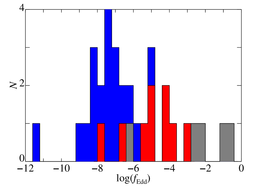
Figure 3.— Histogram of Eddington fractions defined as $f_{\mathrm{Edd}}=L_{X}/L_{\mathrm{Edd}}$. The contribution to the histogram from Seyfert galaxies is colored red, from other SMBH sources is colored blue, and from stellar-mass sources considered in section 5.3 is colored gray. The galaxy with the smallest $f_{\mathrm{Edd}}$ is Sgr A*. A wide range of values are present in the sample even if most are found between $f_{\mathrm{Edd}}=10^{-9}$ and $10^{-6}$. As expected, galaxies classified as Seyferts are, on average, emitting at a higher fraction of Eddington than other sources, and the stellar-mass sources are emitting at a higher fraction still.

4. Analysis

4.1. Fitting Method

For our measurement of the relation between $M_{\mathrm{BH}}$, $L_{R}$ and $L_{X}$, we considered the form

$$\log{L_{R,38}}=R_{0}+\xi_{m}\log{M_{\mathrm{BH},8}}+\xi_{x}\log{L_{X,40}},$$ (1)

where we have normalized to $L_{R}=10^{38}~{}\mathrm{erg\,s^{-1}}L_{R,38}$, $M_{\mathrm{BH}}=10^{8}{\rm M}_{\scriptscriptstyle\odot}M_{\mathrm{BH},8}$, and $L_{X}=10^{40}L_{X,40}$ in order to minimize intercept errors. To find the multi-parameter relation, we minimized the following statistic

$$\tilde{\chi}^{2}=\sum_{i}{\frac{\left(R_{i}-R_{0}-\xi_{m}\mu_{i}-\xi_{x}X_{i}\right)^{2}}{\sigma_{r,i}^{2}+\xi_{m}^{2}\sigma_{m,i}^{2}+\xi_{x}^{2}\sigma_{x,i}^{2}}},$$ (2)

where $R=\log{L_{R,38}}$, $\mu=\log{M_{\mathrm{BH},8}}$, $X=\log{L_{X,40}}$, and the sum is over each galaxy. The $\sigma$ terms are scatter terms that reflect deviation from the plane due to intrinsic scatter and measurement errors. This statistic is the same statistic used by Merloni et al. (2003). We considered two cases. For the first, we assume that the intrinsic scatter is dominant and isotropic and thus use a total scatter projected in to the $R$ direction: $\sigma_{0}^{2}=\sigma^{2}_{r,i}+\xi_{m}^{2}\sigma^{2}_{m,i}+\xi_{x}^{2}\sigma^{2}_{x,i}$. To determine $\sigma_{0}$, we use a trial value of $\sigma_{0}$ and increase the value until the reduced $\chi^{2}$ is unity after fitting with the new value. For the second, we use the measurement errors in $M_{\mathrm{BH}}$ and $L_{X}$, assumed to be normally distributed in logarithmic space, for $\sigma_{m}$ and $\sigma_{x}$ respectively. The measurement errors in $L_{R}$ are likely the smallest, and thus intrinsic scatter is likely to dominate. Here we assume $\sigma_{r}=\sigma_{0}$. In this final case, our fit method is no longer symmetric, but it includes measurement errors and does not assume that the intrinsic scatter is isotropic. Both methods give nearly identical results, and we report only results from the latter method, which includes measurement errors. The errors on fit parameters come from the formal covariance matrix of the fit.

4.2. Fundamental Plane Slopes

Our best-fit relation for the fundamental plane is

$$R_{0} = -0.34\pm 0.24$$

$$\xi_{m} = \phantom{-}0.78\pm 0.27$$

$$\xi_{x} = \phantom{-}0.67\pm 0.12.$$ (3)

The scatter we find in the $L_{R}$ direction is $\sigma_{0}=1.00\ \mathrm{dex}$, equivalent to 0.70 dex normal to the plane. These results are consistent with the findings of Merloni et al. (2003) and of Falcke et al. (2004). We plot several views of the fundamental plane in Figure 4 and the edge-on view in Figure 5. It is also interesting to note that for a fixed value of $M_{\mathrm{BH}}$ our relation finds $L_{R}\propto L_{X}^{0.67}$, consistent with the findings of Gallo et al. (2003).

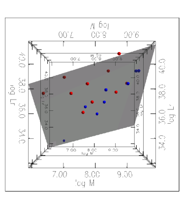
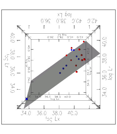
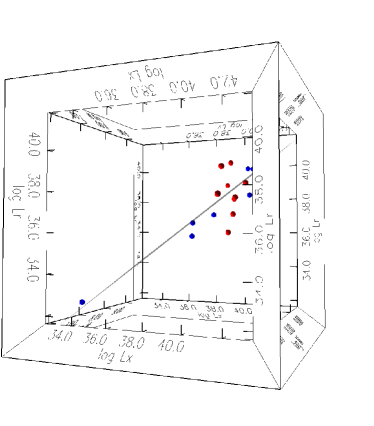
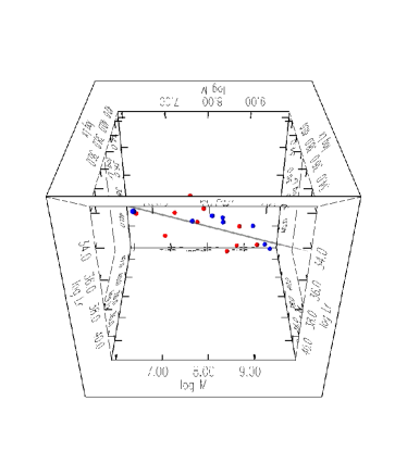
Figure 4.— Four views of the fundamental plane. Data are as described in Sections 2 and 3. Red points are galaxies classified as Seyferts. Blue points are LLAGNs and LINER galaxies. The varying views clearly show that as a whole the points lie on a plane in the dimensions shown. It is especially clear in the top-right panel that the LLAGN/LINER subsample appear to lie on a one-dimensional manifold.

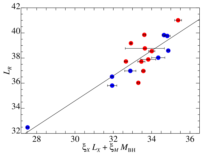
Figure 5.— The fundamental plane relation. This figure shows the edge-on view of our best-fit relation: $\xi_{m}=0.78$ and $\xi_{x}=0.67$. Error bars on the $x$-axis are calculated as $\sigma^{2}_{i}=\xi^{2}_{m}\sigma^{2}_{m,i}+\xi^{2}_{x}\sigma^{2}_{x,i}$. This view is primarily for comparison with Merloni et al. (2003) and with Falcke et al. (2004). Red circles are Seyferts. Blue circles are LINERs and unclassivied LLAGN.

4.3. $M_{\mathrm{BH}}$ as the Dependent Variable

We are using black hole masses that have been measured directly. This approach allows us to use $L_{R}$ and $L_{X}$ as predictor variables for $M_{\mathrm{BH}}$. We perform a multivariate linear regression on $L_{R}$ and $L_{X}$by assuming a form

$$\log M_{\mathrm{BH},8}=\mu_{0}+c_{r}\log L_{R,38}+c_{x}\log L_{X,40}$$ (4)

and minimizing

$$\chi^{2}=\sum_{i}\frac{\left(\mu_{i}-\mu_{0}-c_{r}R-c_{x}X\right)^{2}}{\sigma^{2}_{m,i}+\sigma^{2}_{0}},$$ (5)

where $\sigma_{m,i}$ is the measurement error in $M_{\mathrm{BH}}$ and $\sigma_{0}$ is an intrinsic scatter term in the $\log(M_{\mathrm{BH}})$ direction. As before, the intrinsic scatter term is increased until the resulting best fit gives $\chi^{2}=1$. We find a best-fit relation of

$$\mu_{0} = \phantom{-}0.19\pm 0.19$$

$$c_{r} = \phantom{-}0.48\pm 0.16$$

$$c_{x} = -0.24\pm 0.15,$$ (6)

with an intrinsic scatter of $\sigma_{0}=0.77\ \mathrm{dex}$ in the mass direction. The intrinsic scatter is larger than other scaling relations (e.g., $\sigma_{0}=0.44\pm 0.06$ for the $M$–$\sigma$ relation and $\sigma_{0}=0.38\pm 0.09$ for the $M$–$L$ relation; Gültekin et al. 2009b). We plot projections of fit in the left panel of Figure 6.

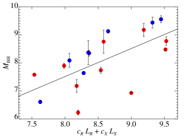
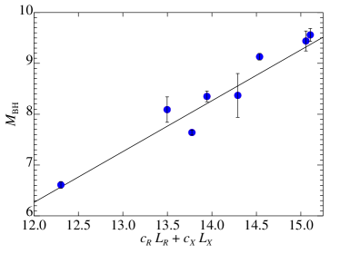
Figure 6.— Best fit linear regression of $M_{\mathrm{BH}}$ on $L_{R}$ and $L_{X}$ for (left) all galaxies and for (right) LLAGN and LINER galaxies only. The relation on the right is considerably tighter but may be affected by the small number of sources. Red circles are Seyferts. Blue circles are LINERs and unclassivied LLAGN.

5. Discussion

5.1. Using A Black Hole’s Luminosity to Estimate Its Mass

By using a sample of galaxies that have directly measured black hole masses, we are able to investigate the correlation between X-ray and radio luminosity and black hole mass. The measure of any correlation’s worth as a predictor is the scatter, and we consider the scatter here. The scatter in the full relation is considerable ($0.77\ \mathrm{dex}=5.9$), but it is only a factor of a couple larger than other scaling relations used to estimate black hole mass. For example the $M$–$\sigma$ and $M$–$L$ relations that relate $M_{\mathrm{BH}}$ and host galaxy velocity dispersion and bulge luminosity have intrinsic scatters of $0.44\ \mathrm{dex}=2.75$ and $0.38\ \mathrm{dex}=2.4$, respectively (Gültekin et al., 2009b).

It is worth noting that if we restrict the sample to just black holes with mass $M_{\mathrm{BH}}>3\times 10^{7}$ or $M_{\mathrm{BH}}>10^{8}\ {\rm M}_{\scriptscriptstyle\odot}$, the intrinsic scatter drops to $\sigma_{0}=0.45$ or $0.41$, respectively. There are several possible interpretations for the decreased scatter when restricting the sample by mass. One possibility is that the requirement of detection in both radio and X-rays translates to a requirement of high Eddington fraction for low-mass black holes at a fixed distance. The mean values of $f_{\mathrm{Edd}}$ for the whole sample, for the sample with $M_{\mathrm{BH}}>3\times 10^{7}{\rm M}_{\scriptscriptstyle\odot}$, and for the sample with $M_{\mathrm{BH}}>10^{8}{\rm M}_{\scriptscriptstyle\odot}$ are approximately $6\times 10^{-5}$, $6\times 10^{-6}$, and $3\times 10^{-6}$, respectively. It is possible that when sources accrete at a higher rate, the fundamental plane relation may no longer apply.

Another possible explanation for the smaller scatter in the high-mass sample is that the low-scatter trend is real, and that the scatter estimated from the entire sample is skewed by a few data points. The most obvious outliers from the left panel of Figure 6 are Circinus and NGC 1068. If these two are eliminated, the scatter becomes $\sigma_{0}=0.50\ \mathrm{dex}$. The derived intrinsic luminosities of these sources may be difficult to determine because of obscuration. In these sources we have a poor view of the central engine and are seeing reflected, rather than direct X-ray emission (Matt et al., 1996; Antonucci & Miller, 1985). If the intrinsic X-ray luminosity of these sources is higher, then they would lie closer to the best-fit plane than they do now.

AGN classification for each galaxy of the sample is listed in Table The Fundamental Plane of Accretion onto Black Holes with Dynamical Masses. The distinction between Seyferts and LINERs is judged from the line ratios with the usual diagnostic and division set so that Seyferts have [OIII]$\lambda$5007/H$\beta>3.0$ (Veilleux & Osterbrock, 1987) as a measurement of the level of nuclear ionization, though there is no obvious transition between the two classes (Ho et al., 2003). The physical difference between LINERs and Seyferts may be that the LINERs lack a “big blue bump” and produce a larger partially ionized zone. The transition in spectral energy distribution from a Seyfert to a LINER may happen at low $f_{\mathrm{Edd}}$ (Ho, 2008). The distinction between Seyfert types is determined by the ratio of broad-line and narrow-line emission. LLAGN are defined by having an H$\alpha$ luminosity smaller than $L(H\alpha)\leq 10^{40}~{}\mathrm{erg\,s^{-1}}$ (Ho et al., 1997). The difference between Seyfert types is understood to be due to differing viewing angles with respect to an obscuring dusty torus that surrounds the broad line region (with type 1 unobscured and type 2 completely obscured). For a review of the observational differences among the different classes and the current physical explanations for the differences see the review by Ho (2008).

We may give special consideration to all non-Seyfert AGNs in our sample. Since all Seyferts in our sample are at least partially obscured, obscuration is one potential issue that is addressed. Obscuration will naturally lead to an underestimate in X-ray luminosity. We minimize this by fitting for the absorption across the 0.5–10 keV band. Since the softer photons are more readily absorbed, the shape of the spectrum gives an indication of the level of absorption. We also use the hard X-ray flux, which is least affected by absorption, for our X-ray luminosity. Nevertheless, the most heavily obscured sources may be intrinsically brighter than our fits indicate. We attempt to isolate this issue below by removing Compton-thick sources. In addition to obscuration, as mentioned above, Seyferts also accrete at higher fractions of Eddington and may accrete in a mode different from LINERs. In addition, since Seyferts are thought to be dominated by thermal output, their radio luminosities may be poor probes of the power in outflows and thus not belong on the relation considered here. Thus, there is a physical motivation to separate them from the rest of the sample.

When we only use the 8 LINER and unclassified LLAGN sources, our fit becomes

$$\mu_{0} = \phantom{-}0.70\pm 0.11$$

$$c_{r} = \phantom{-}0.48\pm 0.14$$

$$c_{x} = -0.07\pm 0.12,$$ (7)

with a scatter of $\sigma_{0}=0.25$, substantially smaller than other intrinsic scatter measurements found for this relation and actually smaller than the scatter in the $M$–$\sigma$ and $M$–$L$ relations. Körding et al. (2006) similarly found a substantially reduced scatter in fundamental plane fits to a sample of only stellar-mass black holes, Sgr A*, and LLAGNs. The fit we find is significantly different from the other fits, notably that it is consistent with no dependence on X-ray luminosity ($c_{x}=0$). This is at odds with the findings of Ho (2002), who found no dependence of black hole mass on radio luminosity. The data do appear to lie on a one-dimensional manifold in the three-dimensional space considered, but with only 8 data points, the data set is substantially smaller than that of Ho (2002), who also used direct, primary mass measurements in addition to direct, secondary mass measurements (i.e., reverberation mapping).

If obscuration, rather than accretion rate or accretion mode, is the underlying reason for the smaller scatter in the LINER/LLAGN sample, then we should see similar results when omitting sources that are Compton thick ($n_{H}\geq\sigma_{T}^{-1}=1.5\times 10^{24}\ \mathrm{cm^{-2}}$). Compton-thick sources will be heavily obscured and the intrinsic luminosities may be much higher than the observed flux would imply (Levenson et al., 2002, 2006). If we conservatively omit the sources from Table 2 intrinsic absorption larger than $10^{24}\ \mathrm{cm^{-2}}$ (NGC 3031, NGC 4374, and NGC 6251) as well as the sources determined to be Compton thick from Fe K$\alpha$ modeling (Circinus and NGC 1068; Levenson et al., 2002, 2006), we obtain

$$\mu_{0} = \phantom{-}0.40\pm 0.16$$

$$c_{r} = \phantom{-}0.46\pm 0.13$$

$$c_{x} = -0.14\pm 0.12,$$ (8)

with a scatter of $\sigma_{0}=0.53$. This result is consistent with the Seyfertless sample at about the 1$\sigma$ level, though with a larger scatter.

5.2. Sgr A*

Sgr A*, the central black hole in the Galaxy, is a unique source in many ways. Its extremely low accretion rate ($L_{X}/L_{\mathrm{Edd}}\approx 4\times 10^{-12}$) is two orders of magnitude below the next lowest in our sample. An analog to Sgr A* could not be observed outside of the local group.

When using only the two nearby super-massive black holes with extremely well-determined mass and distance (Sgr A* and NGC 4258) and the X-ray binary in which the correlation extends over several orders of magnitude (GX 339$-$4), the best-fit fundamental plane relation changes so that Sgr A* is under-luminous in X-rays during quiescence by at least 2 orders of magnitude (Markoff, 2005). Such a break from the correlation (also seen in some X-ray binaries as they rise out of quiescence Coriat et al., 2009) may indicate that, during quiescence at least, Sgr A* is accreting in a different mode than the correlation sources. If such an extremely low accretion rate is in a different category from the rest of the objects, then it makes sense to exclude Sgr A* from the sample, in which case our best fit becomes

$$R_{0} = -0.46\pm 0.30$$

$$\xi_{m} = \phantom{-}0.84\pm 0.29$$

$$\xi_{x} = \phantom{-}0.80\pm 0.23,$$ (9)

with an intrinsic scatter of $\sigma_{0}=1.02$, which is not a significantly different fit.

5.3. Stellar-mass Sources

Our initial sample includes only the supermassive black holes in galactic centers. There are, however, several Galactic stellar-mass black holes with dynamically measured masses. If accretion onto black holes is driven by the same physical processes at all mass scales, then the stellar-mass sources should obey the same relation, which is what Merloni et al. (2003) and Falcke et al. (2004) found. So while our focus has been on super-massive black holes, we may revisit our calculations with the sample of stellar-mass black holes given in Table 5.3. This sample was selected from stellar-mass black holes with dynamically determined masses with simultaneous X-ray and radio data. In addition to the sources listed, there were two stellar mass black holes that had adequate data (4U 1543$-$475 and GRO J1655$-$40) but whose jets may not be in a steady state and thus skewing the relation.

The stellar-mass systems, with the possible exception of GRS 1915, are in the low/hard state, which is characterized by a hard X-ray photon index ($1.4<\Gamma<2.1$), a small ratio of unabsorbed disk flux to total unabsorbed flux ($f<0.2$; Remillard & McClintock, 2006) and is usually seen at low Eddington rates. This state is also typically associated with a steady radio jet whereas jets in the high/soft state are quenched (Fender, 2001). By requiring radio emission, we essentially require a low/hard state. If such a state can be extended to SMBH sources, it would naturally compare with the similarly low Eddington rates in LLAGNs in which jet emission is more prominent compared to Seyferts. The mapping of X-ray binary states to accreting SMBHs is complicated by the fact that no comparable transitions are seen in SMBHs.

These three accreting black holes have masses measured from period measurements of the donor star’s orbit. The mass of the donor star is estimated based on spectral type, and the inclination of the orbit for systems such as these is generally derived from modeling the star’s change in flux, assumed to be from the change in viewing angle of a tear-drop-shaped object (ellipsoidal modulation). For two of the three stellar-mass sources we are using, however, the inclination is constrained by other means. For GRS 1915+105 the inclination is constrained from the apparent superluminal motion of ejected jet material that is assumed to be perpendicular to the orbital plane based on the lack of observed precession (Mirabel & Rodríguez, 1994; Greiner et al., 2001b). For Cyg X-1, the inclination has been estimated in several ways, including UV line modeling and X-ray polarization (Ninkov et al., 1987, and references therein).

The luminosity data from each source is simultaneous, which is important for these highly variable sources. For two of the sources, we use two sets of simultaneous observations. Using more than one observation of a particular source in the fit over-weights that source and will skew the fit if it is atypical. Under the assumption that each source belongs in the fit in all of the epochs used, however, they provide valuable extra information of possible accretion states in the same relation.

Table 1Stellar-Mass Black Hole Data

Name	$D$	$\log\left(M_{\mathrm{BH}}\right)$		$\log\left(L_{R}\right)$	$\log\left(L_{X}\right)$		Refs.
GRS 1915+105	11	1.15$\pm$	0.13	30.64	38.06$\pm$	0.06	1,2,3,3
…	11	1.15$\pm$	0.13	30.90	38.69$\pm$	0.06	1,2,3,3
V404 Cyg	3	1.08$\pm$	0.07	28.30	33.07$\pm$	0.24	4,4,5,6
Cygnus X-1	2.5	1.00$\pm$	0.24	29.91	36.71$\pm$	0.18	7,8,9
…	2.5	1.00$\pm$	0.24	29.84	36.77$\pm$	0.18	7,8,9

Note. — Stellar-mass black hole data used in section 5.3. Distances are given in units of $\mathrm{kpc}$. Black hole masses are in solar units. Radio and X-ray luminosities are in units of $\mathrm{erg\ s^{-1}}$. All values are scaled to the distances given. The sources were in low/hard state for the epochs listed with the exception of GRS 1915, which may be in a plateau state (Muno et al., 2001). The numbers in the reference column give the number of the original reference for the distance, mass, radio luminosity, and X-ray luminosity, respectively. X-ray luminosities have been converted to the $E=2$–$10\ \mathrm{keV}$ band.

References. — (1) Fender et al. 1999; (2) Greiner et al. 2001a; (3) Muno et al. 2001; (4) Shahbaz et al. 1994; (5) Gallo et al. 2005a; (6) Bradley et al. 2007; (7) Bregman et al. 1973; (8) Herrero et al. 1995; (9) Stirling et al. 2001.

The results of our fundamental plane fits become:

$$R_{0} = -0.33\pm 0.21$$

$$\xi_{m} = \phantom{-}0.82\pm 0.08$$

$$\xi_{x} = \phantom{-}0.62\pm 0.10,$$ (10)

with an intrinsic scatter of $\sigma_{0}=0.88$. The uncertainties in slopes have decreased because of the increased range in the values present, especially for $\xi_{m}$. It is interesting to note that while the best-fit parameters do not significantly change from our fits to central black holes, the intrinsic scatter does. This decrease can be attributed to the fact that these sources lie closer to the plane. It is also worth noting that the fits do not change even though two of the stellar-mass sources are accreting at a much higher fraction of Eddington than the supermassive sources. GRS 1915+105 is accreting at $f_{\mathrm{Edd}}\approx 0.06$ to $0.3$, and Cygnus X-1 at $f_{\mathrm{Edd}}\approx 0.004$ to $0.005$, whereas all of the supermassive sources are accreting at $f_{\mathrm{Edd}}<0.001$ (Fig. 3).

It should be noted that there are different systematic errors in the stellar-mass and central black holes. The mass measurements are from completely different methods. The X-ray extragalactic sources may be contaminated from point sources and may be more heavily obscured than the stellar-mass sources. The extragalactic sources may also be contaminated by supernova remnants along the line of sight, though this can be mitigated by going to higher frequencies. Stellar mass uncertainties are dominated by uncertainties in distance, inclination, and light from accretion (see Reynolds et al., 2008).

5.4. Future Work

In this paper, we have only included the 18 black holes with measured masses, radio fluxes, and X-ray fluxes. This sample makes up slightly more than one third of the entire sample of black holes with measured masses. There are 11 without nuclear radio data or only with upper limits on one or more of these quantities. There are a further 16 sources with no Chandra X-ray fluxes measured because either there are no Chandra data or merely insufficient data. Many of the sources have masses $M<10^{8}\,{\rm M}_{\scriptscriptstyle\odot}$. By completing the sample of $M$–$\sigma$ black holes with further X-ray and radio observations, the increased number of data points should be especially helpful in determining whether the large scatter at the low-mass end and the small scatter at the high-mass end are actual differences or just artifacts of a few outliers.

Another place for future work is in understanding the apparent special place that Seyfert galaxies occupy in the fundamental plane. If one were to naïvely assign accretion states used for stellar-mass black holes to Seyfert galaxies, they would be considered in the thermally dominant/high–soft state. For stellar-mass black holes in this state, jets are not measured. That the Seyfert galaxies are an apparent source of scatter in the relation may be an indication that they are diverging away from the fundamental plane relation. To better understand the differences between Seyfert galaxies and the other sources, a future theoretical work will consider just these types of sources, including physical modeling of the data sets presented here.

6. Conclusions

In this paper we analyze the relationship among X-ray luminosity, radio luminosity, and the mass of a black hole. Distinct from previous studies of this relationship, we use only black hole masses that have been dynamically measured. Because of the relatively small distances to the objects in this sample, we avoid potential biases arising from flux limited samples. Using the most recent compilation of black hole masses, we analyzed archival Chandra data to get nuclear X-ray luminosities in the $E=2$–$10\ \mathrm{keV}$ band. We combined this with $\nu=5\ \mathrm{GHz}$ radio luminosities found in the literature and fit a relation of the form $L_{R,38}=R_{0}+\xi_{m}\log M_{\mathrm{BH},8}+\xi_{x}\log L_{X,40}$ to find

$$R_{0} = -0.34\pm 0.24$$

$$\xi_{m} = \phantom{-}0.78\pm 0.27$$

$$\xi_{x} = \phantom{-}0.67\pm 0.12$$ (11)

with a scatter of $\sigma=1.00$ in the $\log L_{R}$ direction, consistent with previous work. We also fit a relation to be used as an estimation for black hole mass based on observations of $L_{X}$ and $L_{R}$of the form:

$$\log M_{\mathrm{BH},8}=\mu_{0}+c_{r}\log L_{R,38}+c_{x}\log L_{X,40},$$ (12)

finding

$$\mu_{0} = \phantom{-}0.19\pm 0.19$$

$$c_{r} = \phantom{-}0.48\pm 0.16$$

$$c_{x} = -0.24\pm 0.15,$$ (13)

with an intrinsic scatter of $\sigma_{0}=0.77$ in the $\log M_{\mathrm{BH}}$ direction. This intrinsic scatter is larger than other scaling relations involving $M_{\mathrm{BH}}$, but decreases considerably when only using the most massive black holes or when eliminating obscured central engines from the sample. Both of these issues require further investigation and could be answered by completing the sample with more Chandra observations.

Table 2Summary of Chandra Spectral Fits

Galaxy	Obs. ID	Exp.	$\chi^{2}/\nu$	Galactic absorption	Intrinsic absorption		Power-law		APEC		Gaussian
		[ks]		$n_{H}$ [$\mathrm{cm}^{-2}$]	$n_{H}$ [$\mathrm{cm}^{-2}$]	$f_{\mathrm{cov}}$	$\Gamma$	$A_{\mathrm{pl}}$	$kT_{\mathrm{APEC}}$ [$\mathrm{keV}$]	$A_{\mathrm{APEC}}$	$E_{\mathrm{line}}$ [$\mathrm{keV}$]	$\sigma_{\mathrm{line}}$ [$\mathrm{keV}$]	$A_{\mathrm{line}}$
Circinus	356	24.7	$261.9/166$	$1.88^{+0.05}_{-0.07}\times 10^{22}$	…	…	$-1.39_{-0.14}^{+0.10}$	$1.40^{+0.12}_{-0.26}\times 10^{-4}$	$1.00_{-0.04}^{+0.05}$	$2.96^{+0.18}_{-0.25}\times 10^{-2}$	$6.40_{-0.00}^{+0.00}$	$3.41^{+0.82}_{-0.96}\times 10^{-2}$	$2.87^{+0.13}_{-0.15}\times 10^{-3}$
CygnusA	1707	9.2	$143.6/112$	$1.99^{+0.57}_{-0.47}\times 10^{21}$	$1.47^{+0.07}_{-0.07}\times 10^{23}$	$0.98_{-0.00}^{+0.00}$	$1.34_{-0.08}^{+0.09}$	$3.04^{+0.51}_{-0.41}\times 10^{-3}$	…	…	$6.07_{-0.02}^{+0.02}$	$7.06^{+2.22}_{-2.61}\times 10^{-2}$	$8.47^{+1.41}_{-1.35}\times 10^{-5}$
IC1459	2196	58.8	$189.5/178$	$2.13^{+0.12}_{-0.12}\times 10^{21}$	…	…	$1.96_{-0.04}^{+0.04}$	$2.35^{+0.09}_{-0.08}\times 10^{-4}$	…	…	…	…	…
IC4296	3394	24.8	$85.6/74$	$1.40^{+0.27}_{-0.22}\times 10^{21}$	…	…	$0.80_{-0.08}^{+0.08}$	$3.24^{+0.36}_{-0.33}\times 10^{-5}$	$0.55_{-0.02}^{+0.02}$	$1.20^{+0.14}_{-0.14}\times 10^{-4}$	…	…	…
N0221	5690	113.0	$19.5/22$	$8.33^{+30.39}_{-8.33}\times 10^{19}$	…	…	$2.01_{-0.11}^{+0.16}$	$6.71^{+1.00}_{-0.49}\times 10^{-6}$	…	…	…	…	…
N0821	6313	49.5	…	$8.53^{+14.85}_{-8.53}\times 10^{20}$	…	…	$2.00_{-0.48}^{+0.56}$	$1.38^{+0.91}_{-0.47}\times 10^{-6}$	…	…	…	…	…
N1023	8464	47.6	$6.4/17$	$1.46^{+0.43}_{-0.45}\times 10^{21}$	…	…	$2.15_{-0.15}^{+0.14}$	$1.80^{+0.34}_{-0.28}\times 10^{-5}$	…	…	…	…	…
N1068	344	47.4	$217.8/125$	$1.32^{+0.10}_{-0.15}\times 10^{21}$	…	…	$3.48_{-0.09}^{+0.09}$	$3.26^{+0.23}_{-0.20}\times 10^{-4}$	$0.80_{-0.02}^{+0.02}$	$7.87^{+0.46}_{-0.70}\times 10^{-5}$	…	…	…
N1399	319	57.4	$17.7/12$	$4.71^{+5.79}_{-2.71}\times 10^{21}$	…	…	$4.62_{-1.98}^{+3.64}$	$<5.68\times 10^{-5}$	…	…	…	…	…
N2787	4689	30.9	$18.6/21$	$1.27^{+0.40}_{-0.41}\times 10^{21}$	…	…	$2.20_{-0.16}^{+0.15}$	$3.53^{+0.57}_{-0.48}\times 10^{-5}$	…	…	…	…	…
N3031	6897	14.8	$119.9/90$	$<1.73\times 10^{20}$	$1.14^{+0.15}_{-0.31}\times 10^{24}$	$0.85_{-0.10}^{+0.07}$	$1.78_{-0.04}^{+0.06}$	$9.62^{+8.42}_{-3.78}\times 10^{-3}$	…	…	…	…	…
N3115	2040	37.0	$5.7/3$	$1.44^{+0.88}_{-1.13}\times 10^{21}$	…	…	$2.35_{-0.68}^{+0.89}$	$5.75^{+4.17}_{-2.19}\times 10^{-6}$	…	…	…	…	…
N3227	860	49.3	$316.5/233$	$<1.29\times 10^{20}$	$8.43^{+1.92}_{-1.93}\times 10^{21}$	$0.53_{-0.08}^{+0.04}$	$0.69_{-0.08}^{+0.05}$	$4.83^{+0.38}_{-0.54}\times 10^{-4}$	…	…	$6.24_{-0.02}^{+0.02}$	$1.81^{+375.39}_{-1.81}\times 10^{-4}$	$1.35^{+0.31}_{-0.31}\times 10^{-5}$
N3245	2926	9.6	…	$1.62^{+1.29}_{-1.18}\times 10^{21}$	…	…	$1.90_{-0.41}^{+0.44}$	$1.13^{+0.59}_{-0.36}\times 10^{-5}$	…	…	…	…	…
N3377	2934	39.6	$1.7/3$	$2.94^{+0.92}_{-1.17}\times 10^{21}$	…	…	$3.14_{-0.65}^{+0.75}$	$1.16^{+0.71}_{-0.42}\times 10^{-5}$	…	…	…	…	…
N3379	7076	69.3	$3.2/4$	$8.19^{+6.83}_{-8.19}\times 10^{20}$	…	…	$2.05_{-0.46}^{+0.39}$	$3.82^{+1.78}_{-1.09}\times 10^{-6}$	…	…	…	…	…
N3384	4692	9.9	…	$3.15^{+1.75}_{-1.87}\times 10^{21}$	…	…	$3.25_{-0.83}^{+0.78}$	$1.80^{+1.32}_{-0.83}\times 10^{-5}$	…	…	…	…	…
N3585	2078	35.3	$19.2/6$	$9.69^{+0.00}_{-0.00}\times 10^{20}$	…	…	$2.09_{-0.00}^{+0.00}$	$8.02^{+0.00}_{-0.00}\times 10^{-6}$	…	…	…	…	…
N3607	2073	38.5	…	$7.90^{+0.34}_{-0.30}\times 10^{21}$	…	…	$7.70_{-1.81}^{+2.23}$	$<6.29\times 10^{-5}$	…	…	…	…	…
N3608	2073	38.5	$0.28/2$	$5.03^{+3.39}_{-1.57}\times 10^{21}$	…	…	$5.59_{-1.61}^{+2.28}$	$<1.02\times 10^{-4}$	…	…	…	…	…
N3998	6781	13.6	$421.7/297$	$5.28^{+6.52}_{-5.28}\times 10^{19}$	…	…	$1.37_{-0.02}^{+0.02}$	$1.52^{+0.03}_{-0.03}\times 10^{-3}$	…	…	…	…	…
N4026	6782	13.8	…	$3.46^{+3.01}_{-2.37}\times 10^{21}$	…	…	$3.47_{-1.13}^{+1.54}$	$7.06^{+10.74}_{-7.06}\times 10^{-6}$	…	…	…	…	…
N4151	335	47.4	$366.7/253$	$<5.12\times 10^{21}$	$7.51^{+26.17}_{-7.51}\times 10^{21}$	$0.05_{-0.05}^{+0.95}$	$-0.92_{-0.06}^{+0.03}$	$4.71^{+0.33}_{-0.41}\times 10^{-5}$	$0.61_{-0.03}^{+0.03}$	$1.06^{+0.00}_{-0.00}\times 10^{-4}$	$6.40_{-0.01}^{+0.01}$	$7.36^{+3886.77}_{-7.36}\times 10^{-5}$	$3.49^{+0.55}_{-0.51}\times 10^{-5}$
N4258	2340	6.9	$67.3/69$	$2.69^{+8.33}_{-1.77}\times 10^{20}$	$6.68^{+0.56}_{-0.48}\times 10^{22}$	$0.99_{-0.00}^{+0.00}$	$1.45_{-0.14}^{+0.17}$	$1.84^{+0.58}_{-0.38}\times 10^{-3}$	…	…	…	…	…
N4261	9569	101.0	$185.8/169$	$9.48^{+1.38}_{-1.35}\times 10^{20}$	$5.32^{+0.79}_{-0.81}\times 10^{20}$	$0.90^{+0.02}_{-0.03}$	$1.35_{-0.10}^{+0.04}$	$1.14^{+0.21}_{-0.24}\times 10^{-4}$	$0.58_{-0.01}^{+0.01}$	$1.38^{+0.08}_{-0.08}\times 10^{-4}$	…	…	…
N4303	2149	28.0	$19.2/8$	$3.09^{+5.56}_{-3.09}\times 10^{20}$	…	…	$2.14_{-0.28}^{+0.38}$	$9.92^{+3.19}_{-1.67}\times 10^{-6}$	…	…	…	…	…
N4342	4687	38.3	$6.2/5$	$<5.39\times 10^{20}$	…	…	$1.44_{-0.17}^{+0.29}$	$5.73^{+1.88}_{-0.52}\times 10^{-6}$	…	…	…	…	…
N4374	803	28.5	$18.2/28$	$2.01^{+0.45}_{-0.42}\times 10^{21}$	$3.74^{+399.93}_{-0.39}\times 10^{24}$	$1.00_{-0.73}^{+0.00}$	$2.20_{-0.17}^{+0.18}$	$4.29^{+0.21}_{-0.33}\times 10^{-2}$	…	…	…	…	…
N4459	2927	9.8	…	$2.55^{+1.34}_{-1.37}\times 10^{21}$	…	…	$3.22_{-0.64}^{+0.65}$	$2.06^{+1.12}_{-0.78}\times 10^{-5}$	…	…	…	…	…
N4473	4688	29.6	…	$9.84^{+14.56}_{-9.84}\times 10^{20}$	…	…	$2.33_{-0.54}^{+0.65}$	$3.85^{+2.47}_{-1.34}\times 10^{-6}$	…	…	…	…	…
N4486	2707	98.7	$344.6/216$	$5.91^{+13.02}_{-5.91}\times 10^{19}$	…	…	$0.81_{-0.03}^{+0.03}$	$4.71^{+0.19}_{-0.16}\times 10^{-5}$	…	…	…	…	…
N4486A	8063	5.1	…	$7.95^{+7.48}_{-4.95}\times 10^{21}$	…	…	$6.14_{-2.60}^{+6.14}$	$<4.81\times 10^{-4}$	…	…	…	…	…
N4564	4008	17.9	…	$1.25^{+10.64}_{-1.25}\times 10^{20}$	…	…	$1.93_{-0.25}^{+0.47}$	$6.53^{+2.99}_{-1.05}\times 10^{-6}$	…	…	…	…	…
N4594	1586	18.5	$110.4/102$	$2.23^{+0.47}_{-0.35}\times 10^{21}$	$2.29^{+0.91}_{-0.91}\times 10^{22}$	$0.39_{-0.22}^{+0.19}$	$1.83_{-0.24}^{+0.31}$	$3.93^{+2.49}_{-1.22}\times 10^{-4}$	…	…	…	…	…
N4596	2928	9.2	…	$2.70^{+5.94}_{-2.70}\times 10^{21}$	…	…	$4.08_{-1.80}^{+4.38}$	$5.28^{+19.72}_{-5.28}\times 10^{-6}$	…	…	…	…	…
N4649	8182	52.4	$30.8/37$	$1.54^{+1.25}_{-1.25}\times 10^{21}$	…	…	$2.45_{-0.60}^{+0.69}$	$1.11^{+0.82}_{-0.45}\times 10^{-5}$	…	…	…	…	…
N4697	784	41.4	$3.2/2$	$<4.20\times 10^{20}$	…	…	$1.81_{-0.27}^{+0.36}$	$2.82^{+0.47}_{-0.17}\times 10^{-6}$	…	…	…	…	…
N4945	864	50.9	$19.4/15$	$1.04^{+0.53}_{-0.35}\times 10^{23}$	$1.27^{+0.00}_{-1.27}\times 10^{24}$	$0.78_{-0.78}^{+0.22}$	$0.48_{-0.88}^{+1.41}$	$6.63^{+151.41}_{-5.97}\times 10^{-5}$	…	…	$6.20_{-0.01}^{+0.01}$	$6.83^{+2.76}_{-2.16}\times 10^{-2}$	$5.64^{+26.35}_{-3.71}\times 10^{-5}$
N5128	3965	49.5	$255.8/200$	$5.96^{+0.59}_{-0.53}\times 10^{22}$	…	…	$-0.05_{-0.11}^{+0.12}$	$8.45^{+2.18}_{-1.59}\times 10^{-5}$	…	…	…	…	…
N5252	4054	60.1	$676.7/445$	$0.00^{+0.00}_{-0.00}\times 10^{19}$	$1.94^{+0.06}_{-0.05}\times 10^{22}$	$0.97_{-0.00}^{+0.00}$	$0.84_{-0.02}^{+0.03}$	$7.52^{+0.36}_{-0.10}\times 10^{-4}$	…	…	…	…	…
N5845	4009	30.0	$0.4/2$	$2.56^{+0.99}_{-1.48}\times 10^{21}$	…	…	$2.52_{-0.76}^{+0.86}$	$9.87^{+7.65}_{-4.12}\times 10^{-6}$	…	…	…	…	…
N6251	4130	45.4	$456.4/358$	$9.73^{+0.57}_{-0.57}\times 10^{20}$	$2.22^{+0.66}_{-0.79}\times 10^{24}$	$0.90_{-0.21}^{+0.09}$	$1.56_{-0.02}^{+0.02}$	$9.68^{+10.35}_{-6.44}\times 10^{-3}$	…	…	…	…	…
N7052	2931	9.6	$16.2/5$	$2.68^{+0.00}_{-0.00}\times 10^{21}$	…	…	$3.81_{-0.00}^{+0.00}$	$5.41^{+0.00}_{-0.00}\times 10^{-5}$	…	…	…	…	…
N7457	4697	9.0	…	$9.78^{+43.94}_{-9.78}\times 10^{20}$	…	…	$2.97_{-1.13}^{+2.37}$	$2.04^{+6.92}_{-2.04}\times 10^{-6}$	…	…	…	…	…
N7582	436	13.4	$131.8/95$	$<1.03\times 10^{20}$	$1.40^{+0.09}_{-0.08}\times 10^{23}$	$0.95_{-0.01}^{+0.01}$	$0.50_{-0.10}^{+0.05}$	$4.14^{+0.38}_{-0.72}\times 10^{-4}$	…	…	…	…	…

Note. — Results from X-ray spectral analysis. First column gives galaxy name. The second column gives Chandra observation identification number. The third column lists exposure time in units of ks. Fourth column lists $\chi^{2}/\nu$ where $\nu$ is the number of degrees of freedom. If the fit used $C$-stat statistics instead of $\chi^{2}$ statistics, then the third column is left blank. Best-fit parameters with 1$\sigma$ errors for each. A blank entry in a given column indicates that the given component was not part of the spectral model used. Galaxies with superscript “a” were only able to constrain an upper limit to the flux. The model for Circinus also included a pileup model.

Table 3Black Hole Data

Galaxy		AGN Class.	$D/\mathrm{Mpc}$	$\log\left(M_{\mathrm{BH}}\right)$		$\log\left(L_{R}\right)$	$\log\left(L_{X}\right)$		Ref.
Circinus	*	S2	4.0	6.23$\pm$	0.088	37.73	41.48$\pm$	0.034	1,2
IC 1459	*	S3	30.9	9.44$\pm$	0.196	39.76	40.86$\pm$	0.014	3,4
IC 4296	*		54.4	9.13$\pm$	0.065	38.59	41.31$\pm$	0.044	5,6
Sgr A*	*		0.008	6.61$\pm$	0.064	32.48	33.33$\pm$	0.068	7,8
NGC 0221			0.9	6.49$\pm$	0.088	…	36.17$\pm$	0.059	9
NGC 0224		S3	0.8	8.17$\pm$	0.161	32.14	$<36.00$		10,11
NGC 0821			25.5	7.63$\pm$	0.157	…	38.44$\pm$	0.640	12
NGC 1023			12.1	7.66$\pm$	0.044	…	38.80$\pm$	0.066	13
NGC 1068	*	S2	15.4	6.93$\pm$	0.016	39.18	39.54$\pm$	0.024	14,15
NGC 1300			20.1	7.85$\pm$	0.289	…	…		16
NGC 1399			21.1	8.71$\pm$	0.060	…	$<38.64$		17
NGC 2748			24.9	7.67$\pm$	0.497	…	…		16
NGC 2778			24.2	7.21$\pm$	0.320	…	…		12
NGC 2787	*	S3b	7.9	7.64$\pm$	0.050	36.52	38.70$\pm$	0.059	18,19
NGC 3031	*	S1.8	4.1	7.90$\pm$	0.087	36.97	40.84$\pm$	0.097	20,21
NGC 3115			10.2	8.98$\pm$	0.182	…	38.04$\pm$	0.312	22
NGC 3227	*	S1.5	17.0	7.18$\pm$	0.228	37.72	41.55$\pm$	0.046	23,21
NGC 3245	*	S3	22.1	8.35$\pm$	0.106	36.98	39.28$\pm$	0.420	23,24
NGC 3377			11.7	8.06$\pm$	0.163	…	38.00$\pm$	0.322	12
NGC 3379	*	S3	11.7	8.09$\pm$	0.250	35.81	38.17$\pm$	0.205	25,26
NGC 3384			11.7	7.25$\pm$	0.042	…	$<38.55$		12
NGC 3585			21.2	8.53$\pm$	0.122	…	38.98$\pm$	0.161	27
NGC 3607		S2	19.9	8.08$\pm$	0.153	…	$<38.60$		27
NGC 3608		S3	23.0	8.32$\pm$	0.173	…	$<38.79$		12
NGC 3998	*	S3b	14.9	8.37$\pm$	0.431	38.03	41.44$\pm$	0.007	28,29
NGC 4026			15.6	8.33$\pm$	0.109	…	$<38.53$		27
NGC 4258	*	S2	7.2	7.58$\pm$	0.001	36.03	40.83$\pm$	0.096	30,21
NGC 4261		S3h	33.4	8.74$\pm$	0.090	39.32	$<40.92$		31,29
NGC 4291			25.0	8.51$\pm$	0.344	…	…		12
NGC 4342			18.0	8.56$\pm$	0.185	…	39.13$\pm$	0.151	32
NGC 4374	*	S2	17.0	9.18$\pm$	0.231	38.77	39.42$\pm$	1.503	33,34
NGC 4459		S3	17.0	7.87$\pm$	0.084	36.13	$<38.97$		18,24
NGC 4473			17.0	8.11$\pm$	0.348	…	$<38.50$		12
NGC 4486	*	S3	17.0	9.56$\pm$	0.126	39.83	40.46$\pm$	0.015	35,36
NGC 4486A			17.0	7.13$\pm$	0.146	…	$<38.96$		37
NGC 4564			17.0	7.84$\pm$	0.045	…	$<38.79$		12
NGC 4594	*	S1.9	10.3	8.76$\pm$	0.413	37.89	40.19$\pm$	0.307	38,39
NGC 4596		S3	18.0	7.92$\pm$	0.162	…	$<38.72$		18
NGC 4649			16.5	9.33$\pm$	0.117	37.45	$<38.95$		12,40
NGC 4697			12.4	8.29$\pm$	0.038	…	38.25$\pm$	0.745	12
NGC 5077		S3b	44.9	8.90$\pm$	0.221	…	…		12
NGC 5128	*	S2?	4.4	8.48$\pm$	0.044	39.85	40.22$\pm$	0.085	41,42
NGC 5576			27.1	8.26$\pm$	0.088	…	…		27
NGC 5845			28.7	8.46$\pm$	0.223	…	39.07$\pm$	0.722	12
NGC 6251	*	S2	106.0	8.78$\pm$	0.151	41.01	42.50$\pm$	0.207	43,44
NGC 7052			70.9	8.60$\pm$	0.223	39.43	$<40.69$		45,46
NGC 7457			14.0	6.61$\pm$	0.170	…	$<38.28$		12
NGC 7582	*	S2	22.3	7.74$\pm$	0.104	38.55	41.69$\pm$	0.208	47,48
PGC 49940			157.5	9.59$\pm$	0.056	…	…		5
Cygnus A		S1.9	257.1	6.43$\pm$	0.126	41.54	44.23$\pm$	0.088	49,6
NGC 4151		S1.5	13.9	7.65$\pm$	0.048	38.20	41.69$\pm$	0.074	50,21
NGC 4303		S2	17.9	6.65$\pm$	0.349	38.46	38.89$\pm$	0.124	51,52
NGC 4742			16.4	7.18$\pm$	0.151	…	…		53
NGC 4945		S	3.7	6.15$\pm$	0.184	38.17	37.80$\pm$	0.921	54,55
NGC 5252		S2	103.7	9.00$\pm$	0.341	39.05	43.20$\pm$	0.017	56,57

Note. — This table lists all galaxies with dynamically measured black hole masses. Sources with an asterisk after their name are those used in this paper. The second column gives AGN classification from Véron-Cetty & Véron (2006) unless it has a superscript “a,” in which case it comes from NED. “S1” indicates type 1 (unobscured) Seyfert, “S2” indicates type 2 (obscured) Seyfert, “S1.X” indicates transitional or intermediate Seyfert, “S3” indicates type 3 Seyfert or LINER galaxy, and “?” indicates that NGC 5128 is a questionable BL Lac object. Note that NGC 3227 and NGC 4151 are classified as type 1.5 but both have reverberation mapping masses (Onken et al., 2003; Bentz et al., 2006) and thus have visible broad-line regions. Beyond these two galaxies, none of the galaxies is obviously a Seyfert 1, though NGC 1068 and NGC 7582 are classified as such by Véron-Cetty & Véron (2006). We classify them according to their NED classifications as Seyfert 2 galaxies. NGC 1068 is a Seyfert 2 galaxy and only shows broad Balmer lines in polarized light, indicating that the light has been scattered and thus coming from behind an obscured source (Antonucci & Miller, 1985). NGC 7582 is a classical Seyfert 2 galaxy that developed broad emission lines for a short period of time in 1998 July (Aretxaga et al., 1999). The change to a Seyfert 1 spectrum may be explained by a stellar disruption event, a change in the obscuring medium, or a type IIn supernova (Aretxaga et al., 1999, see also Véron-Cetty & Véron 2000). It has also been suggested, based on its X-ray spectrum, that NGC 7582 is an obscured narrow-line Seyfert 1 (Dewangan & Griffiths, 2005). For our purposes, we classify this source as a Seyfert 2. The paucity of true Seyfert 1 galaxies in our sample is not surprising since such bright central engines would compromise dynamical black hole mass measurements. The third column gives distance to the galaxy in units of $~{}\mathrm{Mpc}$, which is used to scale all data. The fourth column lists logarithmic black hole mass per unit solar mass as compiled by Gültekin et al. (2009b). The fifth column gives logarithmic radio luminosity in units of $~{}\mathrm{erg\,s^{-1}}$. The radio data come from the compilation of Ho (2002) with the following exceptions: IC 4296, NGC 5128, NGC 7582, NGC 4303, and NGC 5252. The sixth column gives logarithmic X-ray luminosity in units of $~{}\mathrm{erg\,s^{-1}}$, which come from this work except for Sgr A* (Baganoff et al., 2001) and the upper limit on NGC 0224 (Garcia et al., 2005). We leave the column blank if there are no archival data available. The final column lists original references for the $M_{\mathrm{BH}}$ measurement and radio luminosity, if present. The bottom portion of the table gives data for when the black hole mass may be wrong. For this paper we only use data from galaxies that are in the top portion and that have both radio and X-ray detections. Blank entries indicate that there were no archival data available and may be followed up with more observations.

References. — (1) Greenhill et al. 2003, (2) Turner & Ho 1983, (3) Cappellari et al. 2002, (4) Sadler et al. 1989, (5) Dalla Bontà et al. 2008, (6) Sambruna et al. 1999, (7) Ghez et al. 2008 and Gillessen et al. 2008, (8) Ekers et al. 1983, (9) Verolme et al. 2002, (10) Bender et al. 2005, (11) Crane et al. 1992, (12) Gebhardt et al. 2003, (13) Bower et al. 2001, (14) Lodato & Bertin 2003, (15) Ulvestad & Wilson 1984, (16) Atkinson et al. 2005, (17) Gebhardt et al. 2007, (18) Sarzi et al. 2001, (19) Heckman et al. 1980, (20) Devereux et al. 2003, (21) Ho & Ulvestad 2001, (22) Emsellem et al. 1999, (23) Barth et al. 2001, (24) Wrobel & Heeschen 1991, (25) Gebhardt et al. 2000, (26) Fabbiano et al. 1989, (27) Gültekin et al. 2009a, (28) de Francesco et al. 2006, (29) Wrobel & Heeschen 1984, (30) Herrnstein et al. 2005, (31) Ferrarese et al. 1996, (32) Cretton & van den Bosch 1999, (33) Bower et al. 1998, (34) Jenkins et al. 1977, (35) Macchetto et al. 1997, (36) Biretta et al. 1991, (37) Nowak et al. 2007, (38) Kormendy 1988, (39) Hummel et al. 1984, (40) Spencer & Junor 1986, (41) Silge et al. 2005, (42) Wright et al. 1994, (43) Ferrarese & Ford 1999, (44) Jones et al. 1986, (45) van der Marel & van den Bosch 1998, (46) Morganti et al. 1987, (47) Wold et al. 2006, (48) Gregory et al. 1994, (49)   Tadhunter et al. 2003, (50) Onken et al. 2007, (51) Pastorini et al. 2007, (52) Gregory & Condon 1991, (53) listed as in preparation in Tremaine et al. 2002 but never published, (54) Greenhill et al. 1997, (55) Elmouttie et al. 1997, (56) Capetti et al. 2005, (57) Polletta et al. 1996.

References

- Allen et al. (2006) Allen, S. W., Dunn, R. J. H., Fabian, A. C., Taylor, G. B., & Reynolds, C. S. 2006, MNRAS, 372, 21
- Antonucci & Miller (1985) Antonucci, R. R. J., & Miller, J. S. 1985, ApJ, 297, 621
- Aretxaga et al. (1999) Aretxaga, I., Joguet, B., Kunth, D., Melnick, J., & Terlevich, R. J. 1999, ApJ, 519, L123
- Arnaud (1996) Arnaud, K. A. 1996, in Astronomical Society of the Pacific Conference Series 101, Astronomical Data Analysis Software and Systems V, ed. G. H. Jacoby & J. Barnes, 17
- Atkinson et al. (2005) Atkinson, J. W., et al. 2005, MNRAS, 359, 504
- Baganoff et al. (2001) Baganoff, F. K., et al. 2001, Nature, 413, 45
- Bajaja et al. (2005) Bajaja, E., Arnal, E. M., Larrarte, J. J., Morras, R., Pöppel, W. G. L., & Kalberla, P. M. W. 2005, A&A, 440, 767
- Barnes et al. (2006) Barnes, D. G., Fluke, C. J., Bourke, P. D., & Parry, O. T. 2006, Publications of the Astronomical Society of Australia, 23, 82
- Barth et al. (2001) Barth, A. J., Sarzi, M., Rix, H.-W., Ho, L. C., Filippenko, A. V., & Sargent, W. L. W. 2001, ApJ, 555, 685
- Bender et al. (2005) Bender, R., et al. 2005, ApJ, 631, 280
- Bentz et al. (2006) Bentz, M. C., et al. 2006, ApJ, 651, 775
- Biretta et al. (1991) Biretta, J. A., Stern, C. P., & Harris, D. E. 1991, AJ, 101, 1632
- Blandford & Payne (1982) Blandford, R. D., & Payne, D. G. 1982, MNRAS, 199, 883
- Blandford & Znajek (1977) Blandford, R. D., & Znajek, R. L. 1977, MNRAS, 179, 433
- Bower et al. (1998) Bower, G. A., et al. 1998, ApJ, 492, L111
- Bower et al. (2001) ———. 2001, ApJ, 550, 75
- Bradley et al. (2007) Bradley, C. K., Hynes, R. I., Kong, A. K. H., Haswell, C. A., Casares, J., & Gallo, E. 2007, ApJ, 667, 427
- Bregman et al. (1973) Bregman, J., Butler, D., Kemper, E., Koski, A., Kraft, R. P., & Stone, R. P. P. 1973, ApJ, 185, L117+
- Capetti et al. (2005) Capetti, A., Marconi, A., Macchetto, D., & Axon, D. 2005, A&A, 431, 465
- Cappellari et al. (2002) Cappellari, M., Verolme, E. K., van der Marel, R. P., Kleijn, G. A. V., Illingworth, G. D., Franx, M., Carollo, C. M., & de Zeeuw, P. T. 2002, ApJ, 578, 787
- Cash (1979) Cash, W. 1979, ApJ, 228, 939
- Coriat et al. (2009) Coriat, M., Corbel, S., Buxton, M. M., Bailyn, C. D., Tomsick, J. A., Koerding, E., & Kalemci, E. 2009, preprint (0909.3283)
- Crane et al. (1992) Crane, P. C., Dickel, J. R., & Cowan, J. J. 1992, ApJ, 390, L9
- Cretton & van den Bosch (1999) Cretton, N., & van den Bosch, F. C. 1999, ApJ, 514, 704
- Dalla Bontà et al. (2008) Dalla Bontà, E., Ferrarese, L., Corsini, E. M., Miralda-Escudé, J., Coccato, L., Sarzi, M., Pizzella, A., & Beifiori, A. 2008, preprint (0809.0766)
- de Francesco et al. (2006) de Francesco, G., Capetti, A., & Marconi, A. 2006, A&A, 460, 439
- Devereux et al. (2003) Devereux, N., Ford, H., Tsvetanov, Z., & Jacoby, G. 2003, AJ, 125, 1226
- Dewangan & Griffiths (2005) Dewangan, G. C., & Griffiths, R. E. 2005, ApJ, 625, L31
- Ekers et al. (1983) Ekers, R. D., van Gorkom, J. H., Schwarz, U. J., & Goss, W. M. 1983, A&A, 122, 143
- Elmouttie et al. (1997) Elmouttie, M., Haynes, R. F., Jones, K. L., Ehle, M., Beck, R., Harnett, J. I., & Wielebinski, R. 1997, MNRAS, 284, 830
- Emsellem et al. (1999) Emsellem, E., Dejonghe, H., & Bacon, R. 1999, MNRAS, 303, 495
- Fabbiano et al. (1989) Fabbiano, G., Gioia, I. M., & Trinchieri, G. 1989, ApJ, 347, 127
- Fabian et al. (2003) Fabian, A. C., Sanders, J. S., Allen, S. W., Crawford, C. S., Iwasawa, K., Johnstone, R. M., Schmidt, R. W., & Taylor, G. B. 2003, MNRAS, 344, L43
- Falcke & Biermann (1995) Falcke, H., & Biermann, P. L. 1995, A&A, 293, 665
- Falcke et al. (2004) Falcke, H., Körding, E., & Markoff, S. 2004, A&A, 414, 895
- Fender (2001) Fender, R. P. 2001, MNRAS, 322, 31
- Fender et al. (1999) Fender, R. P., Garrington, S. T., McKay, D. J., Muxlow, T. W. B., Pooley, G. G., Spencer, R. E., Stirling, A. M., & Waltman, E. B. 1999, MNRAS, 304, 865
- Ferrarese & Ford (1999) Ferrarese, L., & Ford, H. C. 1999, ApJ, 515, 583
- Ferrarese et al. (1996) Ferrarese, L., Ford, H. C., & Jaffe, W. 1996, ApJ, 470, 444
- Gallo et al. (2005a) Gallo, E., Fender, R. P., & Hynes, R. I. 2005a, MNRAS, 356, 1017
- Gallo et al. (2003) Gallo, E., Fender, R. P., & Pooley, G. G. 2003, MNRAS, 344, 60
- Gallo et al. (2005b) Gallo, E., Fender, R., Kaiser, C., Russell, D., Morganti, R., Oosterloo, T., & Heinz, S. 2005b, Nature, 436, 819
- Garcia et al. (2005) Garcia, M. R., Williams, B. F., Yuan, F., Kong, A. K. H., Primini, F. A., Barmby, P., Kaaret, P., & Murray, S. S. 2005, ApJ, 632, 1042
- Gebhardt et al. (2000) Gebhardt, K., et al. 2000, AJ, 119, 1157
- Gebhardt et al. (2003) ———. 2003, ApJ, 583, 92
- Gebhardt et al. (2007) ———. 2007, ApJ, 671, 1321
- Ghez et al. (2008) Ghez, A. M., et al. 2008, ApJ, 689, 1044
- Gillessen et al. (2008) Gillessen, S., Eisenhauer, F., Trippe, S., Alexander, T., Genzel, R., Martins, F., & Ott, T. 2008, preprint (0810.4674)
- Greenhill et al. (1997) Greenhill, L. J., Moran, J. M., & Herrnstein, J. R. 1997, ApJ, 481, L23
- Greenhill et al. (2003) Greenhill, L. J., et al. 2003, ApJ, 590, 162
- Gregory & Condon (1991) Gregory, P. C., & Condon, J. J. 1991, ApJS, 75, 1011
- Gregory et al. (1994) Gregory, P. C., Vavasour, J. D., Scott, W. K., & Condon, J. J. 1994, ApJS, 90, 173
- Greiner et al. (2001a) Greiner, J., Cuby, J. G., & McCaughrean, M. J. 2001a, Nature, 414, 522
- Greiner et al. (2001b) Greiner, J., Cuby, J. G., McCaughrean, M. J., Castro-Tirado, A. J., & Mennickent, R. E. 2001b, A&A, 373, L37
- Gültekin et al. (2009a) Gültekin, K., et al. 2009a, ApJ, 695, 1577
- Gültekin et al. (2009b) ———. 2009b, ApJ, 698, 198
- Harris et al. (2006) Harris, D. E., Cheung, C. C., Biretta, J. A., Sparks, W. B., Junor, W., Perlman, E. S., & Wilson, A. S. 2006, ApJ, 640, 211
- Hartmann & Burton (1997) Hartmann, D., & Burton, W. B. 1997, Atlas of Galactic Neutral Hydrogen, ed. D. Hartmann & W. B. Burton (Cambridge, UK: Cambridge University Press)
- Heckman et al. (1980) Heckman, T. M., Crane, P. C., & Balick, B. 1980, A&AS, 40, 295
- Heinz & Sunyaev (2003) Heinz, S., & Sunyaev, R. A. 2003, MNRAS, 343, L59
- Herrero et al. (1995) Herrero, A., Kudritzki, R. P., Gabler, R., Vilchez, J. M., & Gabler, A. 1995, A&A, 297, 556
- Herrnstein et al. (2005) Herrnstein, J. R., Moran, J. M., Greenhill, L. J., & Trotter, A. S. 2005, ApJ, 629, 719
- Ho (2002) Ho, L. C. 2002, ApJ, 564, 120
- Ho (2008) ———. 2008, ARA&A, 46, 475
- Ho et al. (1997) Ho, L. C., Filippenko, A. V., & Sargent, W. L. W. 1997, ApJS, 112, 315
- Ho et al. (2003) ———. 2003, ApJ, 583, 159
- Ho & Ulvestad (2001) Ho, L. C., & Ulvestad, J. S. 2001, ApJS, 133, 77
- Hummel et al. (1984) Hummel, E., van der Hulst, J. M., & Dickey, J. M. 1984, A&A, 134, 207
- Jenkins et al. (1977) Jenkins, C. J., Pooley, G. G., & Riley, J. M. 1977, MmRAS, 84, 61
- Jones et al. (1986) Jones, D. L., et al. 1986, ApJ, 305, 684
- Kalberla et al. (2005) Kalberla, P. M. W., Burton, W. B., Hartmann, D., Arnal, E. M., Bajaja, E., Morras, R., & Pöppel, W. G. L. 2005, A&A, 440, 775
- Körding et al. (2006) Körding, E., Falcke, H., & Corbel, S. 2006, A&A, 456, 439
- Kormendy (1988) Kormendy, J. 1988, ApJ, 335, 40
- Levenson et al. (2006) Levenson, N. A., Heckman, T. M., Krolik, J. H., Weaver, K. A., & Życki, P. T. 2006, ApJ, 648, 111
- Levenson et al. (2002) Levenson, N. A., Krolik, J. H., Życki, P. T., Heckman, T. M., Weaver, K. A., Awaki, H., & Terashima, Y. 2002, ApJ, 573, L81
- Li et al. (2009) Li, Z., Wang, Q. D., & Wakker, B. P. 2009, preprint (0902.3847)
- Li et al. (2008) Li, Z.-Y., Wu, X.-B., & Wang, R. 2008, ApJ, 688, 826
- Lodato & Bertin (2003) Lodato, G., & Bertin, G. 2003, A&A, 398, 517
- Lynden-Bell (1978) Lynden-Bell, D. 1978, Phys. Scr, 17, 185
- Macchetto et al. (1997) Macchetto, F., Marconi, A., Axon, D. J., Capetti, A., Sparks, W., & Crane, P. 1997, ApJ, 489, 579
- Markoff (2005) Markoff, S. 2005, ApJ, 618, L103
- Matt et al. (1996) Matt, G., et al. 1996, MNRAS, 281, L69
- McClintock & Remillard (2006) McClintock, J. E., & Remillard, R. A. 2006, Black hole binaries, ed. W. H. G. Lewin & M. van der Klis (Cambridge, UK: Cambridge University Press), 157–213
- McNamara et al. (2006) McNamara, B. R., et al. 2006, ApJ, 648, 164
- Merloni et al. (2003) Merloni, A., Heinz, S., & Di Matteo, T. 2003, MNRAS, 345, 1057
- Merloni et al. (2006) Merloni, A., Körding, E., Heinz, S., Markoff, S., Di Matteo, T., & Falcke, H. 2006, New Astronomy, 11, 567
- Miller et al. (2009) Miller, J. M., Reynolds, C. S., Fabian, A. C., Miniutti, G., & Gallo, L. C. 2009, ApJ, 697, 900
- Mirabel & Rodríguez (1994) Mirabel, I. F., & Rodríguez, L. F. 1994, Nature, 371, 46
- Miyoshi et al. (1995) Miyoshi, M., Moran, J., Herrnstein, J., Greenhill, L., Nakai, N., Diamond, P., & Inoue, M. 1995, Nature, 373, 127
- Morganti et al. (1987) Morganti, R., Fanti, C., Fanti, R., Parma, P., & de Ruiter, H. R. 1987, A&A, 183, 203
- Muno et al. (2001) Muno, M. P., Remillard, R. A., Morgan, E. H., Waltman, E. B., Dhawan, V., Hjellming, R. M., & Pooley, G. 2001, ApJ, 556, 515
- Ninkov et al. (1987) Ninkov, Z., Walker, G. A. H., & Yang, S. 1987, ApJ, 321, 425
- Nowak et al. (2007) Nowak, N., Saglia, R. P., Thomas, J., Bender, R., Pannella, M., Gebhardt, K., & Davies, R. I. 2007, MNRAS, 379, 909
- Onken et al. (2004) Onken, C. A., Ferrarese, L., Merritt, D., Peterson, B. M., Pogge, R. W., Vestergaard, M., & Wandel, A. 2004, ApJ, 615, 645
- Onken et al. (2003) Onken, C. A., Peterson, B. M., Dietrich, M., Robinson, A., & Salamanca, I. M. 2003, ApJ, 585, 121
- Onken et al. (2007) Onken, C. A., et al. 2007, ApJ, 670, 105
- Pastorini et al. (2007) Pastorini, G., et al. 2007, A&A, 469, 405
- Peterson et al. (2004) Peterson, B. M., et al. 2004, ApJ, 613, 682
- Polletta et al. (1996) Polletta, M., Bassani, L., Malaguti, G., Palumbo, G. G. C., & Caroli, E. 1996, ApJS, 106, 399
- Remillard & McClintock (2006) Remillard, R. A., & McClintock, J. E. 2006, ARA&A, 44, 49
- Reynolds et al. (2008) Reynolds, M. T., Callanan, P. J., Robinson, E. L., & Froning, C. S. 2008, MNRAS, 387, 788
- Sadler et al. (1989) Sadler, E. M., Jenkins, C. R., & Kotanyi, C. G. 1989, MNRAS, 240, 591
- Sambruna et al. (1999) Sambruna, R. M., Eracleous, M., & Mushotzky, R. F. 1999, ApJ, 526, 60
- Sarzi et al. (2001) Sarzi, M., Rix, H.-W., Shields, J. C., Rudnick, G., Ho, L. C., McIntosh, D. H., Filippenko, A. V., & Sargent, W. L. W. 2001, ApJ, 550, 65
- Shahbaz et al. (1994) Shahbaz, T., Ringwald, F. A., Bunn, J. C., Naylor, T., Charles, P. A., & Casares, J. 1994, MNRAS, 271, L10
- Sikora et al. (2007) Sikora, M., Stawarz, Ł., & Lasota, J.-P. 2007, ApJ, 658, 815
- Silge et al. (2005) Silge, J. D., Gebhardt, K., Bergmann, M., & Richstone, D. 2005, AJ, 130, 406
- Smith et al. (2001) Smith, R. K., Brickhouse, N. S., Liedahl, D. A., & Raymond, J. C. 2001, ApJ, 556, L91
- Spencer & Junor (1986) Spencer, R. E., & Junor, W. 1986, Nature, 321, 753
- Stirling et al. (2001) Stirling, A. M., Spencer, R. E., de la Force, C. J., Garrett, M. A., Fender, R. P., & Ogley, R. N. 2001, MNRAS, 327, 1273
- Tadhunter et al. (2003) Tadhunter, C., Marconi, A., Axon, D., Wills, K., Robinson, T. G., & Jackson, N. 2003, MNRAS, 342, 861
- Tremaine et al. (2002) Tremaine, S., et al. 2002, ApJ, 574, 740
- Turner & Ho (1983) Turner, J. L., & Ho, P. T. P. 1983, ApJ, 268, L79
- Ulvestad & Wilson (1984) Ulvestad, J. S., & Wilson, A. S. 1984, ApJ, 278, 544
- van der Marel & van den Bosch (1998) van der Marel, R. P., & van den Bosch, F. C. 1998, AJ, 116, 2220
- van Putten (2009) van Putten, M. H. P. M. 2009, preprint (0905.3367)
- Veilleux & Osterbrock (1987) Veilleux, S., & Osterbrock, D. E. 1987, ApJS, 63, 295
- Verolme et al. (2002) Verolme, E. K., et al. 2002, MNRAS, 335, 517
- Véron-Cetty & Véron (2000) Véron-Cetty, M. P., & Véron, P. 2000, A&A Rev., 10, 81
- Véron-Cetty & Véron (2006) Véron-Cetty, M.-P., & Véron, P. 2006, A&A, 455, 773
- Wang et al. (2006) Wang, R., Wu, X.-B., & Kong, M.-Z. 2006, ApJ, 645, 890
- Wold et al. (2006) Wold, M., Lacy, M., Käufl, H. U., & Siebenmorgen, R. 2006, A&A, 460, 449
- Wright et al. (1994) Wright, A. E., Griffith, M. R., Burke, B. F., & Ekers, R. D. 1994, ApJS, 91, 111
- Wrobel & Heeschen (1984) Wrobel, J. M., & Heeschen, D. S. 1984, ApJ, 287, 41
- Wrobel & Heeschen (1991) ———. 1991, AJ, 101, 148
- Yuan & Cui (2005) Yuan, F., & Cui, W. 2005, ApJ, 629, 408
- Yuan et al. (2009) Yuan, F., Yu, Z., & Ho, L. C. 2009, preprint (0902.3704)