Communications in cellular automata

Abstract

The goal of this paper is to show why the framework of communication complexity seems suitable for the study of cellular automata. Researchers have tackled different algorithmic problems ranging from the complexity of predicting to the decidability of different dynamical properties of cellular automata. But the difference here is that we look for communication protocols arising in the dynamics itself. Our work is guided by the following idea : if we are able to give a protocol describing a cellular automaton, then we can understand its behavior.

1 Cellular automata

Throughout this paper we restrict our study to one-dimensional cellular automata. These are infinite collections of cells arranged linearly, each having a state from a finite set. The dynamics of the system is governed by a local rule applied uniformly and synchronously to the lattice of cells.

A cellular automaton (CA) is a triple ${\mathcal{A}=(S,r,f)}$ where:

• $S$ is a (finite) state set,

• $r$ is the neighborhood radius,

• $f:S^{2r+1}\rightarrow S$ is the local transition function.

A coloring of the lattice $\mathbb{Z}$ with states from $S$ (i.e. an element of $S^{\mathbb{Z}}$) is called a configuration. To $\mathcal{A}$ we associate a global function $G$ acting on configurations by synchronous and uniform application of the local transition function. Formally, $G:S^{\mathbb{Z}}\rightarrow S^{\mathbb{Z}}$ is defined by:

$$G(x)_{z}=f(x_{z-r},\ldots,x_{z+r})$$

for all ${z\in\mathbb{Z}}$. Several CA can share the same global function although there are syntactically different (different radii and local functions). However, as we will see below (section 3), the main property we are interested in (namely, communication complexity) is independant of the particular choice of the syntactical representation. Moreover, an important part of the paper (Section 4) focuses on elementary CA, which is a fixed syntactical framework.

After $n$ time steps the value of a cell depends on its own initial state together with the initial states of the $rn$ left and $rn$ right neighbouring cells. More precisely, we define the $n$-th iteration of local rule $f^{n}:\{0,1\}^{2rn+1}\rightarrow\{0,1\}$ recursively: ${f^{1}=f}$ and, for $n\geq 2$,

$$f^{n}(z_{-rn}\ldots z_{1},z_{0},z_{1}\ldots z_{rn})=f^{n-1}(f(z_{-rn},\ldots,z_{-rn+2r})\ldots f(z_{rn-2r},\ldots,z_{rn})).$$

Finally, we call P-complete a cellular automaton such that the problem of predicting $F^{n}$ on all configurations of size $2rn+1$ is P-complete.

Our work is motivated by the following idea: if we are able to give a simple explicit description of $f^{n}$ (for arbitrary $n$), then we can understand the behavior of the corresponding CA.

2 Communication complexity

Communication complexity is a model introduced by A. C.-C. Yao in [17], and designed at first for lower-bounding the amount of communication needed in parallel programs. In this model we consider two players, namely Alice and Bob, each with arbitrary computational power and talking to each other to decide the value of a given function.

For instance, let ${f:X\times Y\rightarrow Z}$ be a function taking pairs as input. If we give first elements of pairs to Alice, and second to Bob, the question communication complexity asks is “how much information do they have to communicate to each other in the worst case in order to compute $f$ ?”.

More precisely, we define protocols, which specify, at each step of the communication between Alice and Bob, who speaks (Alice or Bob), and what he says (a bit, 0 or 1), as a function of their respective inputs.

This simple framework, and some of its variants we discuss in this article, appear to us as a relevant way to study CA. The tools of communication complexity suggest experiments to test hypothesis about properties of CA (see Section 4).

Definition 1.

A protocol $\mathcal{P}$ over domain $X\times Y$ and range $Z$ is a binary tree where each internal node $v$ is labeled either by a map $a_{v}:X\rightarrow\{0,1\}$ or by a map $b_{v}:Y\rightarrow\{0,1\}$, and each leaf $v$ is labeled either by a map ${A_{v}:X\rightarrow Z}$ or by a map ${B_{v}:Y\rightarrow Z}$.

The value of protocol $\mathcal{P}$ on input $(x,y)\in X\times Y$ is given by $A_{v}(x)$ (or $B_{v}(y)$) where $A_{v}$ (or $B_{v}$) is the label of the leaf reached by walking on the tree from the root, and walking left if $a_{v}(x)=0$ (or $b_{v}(y)=0$), and walking right otherwise. We say that a protocol computes a function ${f:X\times Y\rightarrow Z}$ if for any $(x,y)\in X\times Y$, its value on input $(x,y)$ is $f(x,y)$.

Intuitively, each internal node specifies a bit to be communicated either by Alice or by Bob, whereas at leaves either Alice or Bob determines the final value of $f$ since she (or he) has received enough information from the other.

Remark.

In our formalism, we don’t ask both Alice and Bob to be able to give the final value. We do so to be able to consider protocols where communication is unidirectional (see below).

Definition 2.

We denote by $\mathbf{cc}(f)$ the deterministic communication complexity of a function $f:X\times Y\rightarrow Z$. It is the minimal depth of a protocol tree computing $f$.

We study functions with the help of their associated matrices. In such matrices, rows are indexed by elements in $X$, columns by elements in $Y$. They are defined by $M_{i,j}=f(i,j)\in Z$. For elementary CA, we represent the $n$-th iteration function of $f^{n}:\{0,1\}^{2n+1}\rightarrow\{0,1\}$ as $f^{n}:\{0,1\}^{n}\times\{0,1\}^{n+1}\rightarrow\{0,1\}$. For instance, Figure 1 represents the matrix of elementary CA rule 178, when we give $n$ bits to Alice (rows) and $n+1$ bits to Bob (columns); i.e. when $X=\{0,1\}^{n}$ and $Y=\{0,1\}^{n+1}$. We denote as $M_{178}^{n}$ such a matrix.

         

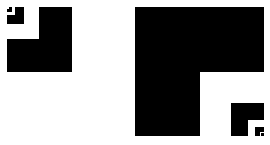
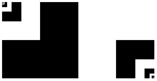
Figure 1: Matrices of rule 178, for $n=6$ (left) and $n=7$ (right)

From the study in [8], we know that a protocol for a function induces a partition of the matrix of this function into monochromatic generalized rectangles (i.e. cartesian products of subsets of $X$ and $Y$). So a lower bound for the deterministic communication complexity of a function $\phi$ is given by $\log_{2}C_{P}(\phi)$, where $C_{P}(\phi)$ stands for the partition number of $\phi$, i.e. the number of rectangles needed in a minimal partition of the matrix into monochromatic rectangles.

Moreover, we call one-round communication complexity, denoted by $\mathbf{cc_{1}}$, the communication complexity when restricted to protocols where only one person (Alice or Bob) can speak. Precisely, a one-round protocol is a tree where either all internal nodes have labels of type $a_{v}$ and all leaves labels of type $B_{v}$ (Alice speaking to Bob who then gives the final answer), or all internal nodes have labels of type $b_{v}$ and all leaves labels of type $A_{v}$ (Bob speaking to Alice who gives the final answer).

Definition 3.

The one-round deterministic communication complexity of a function $f:X\times Y\rightarrow Z$, denoted by $\mathbf{cc_{1}}(f)$, is the minimal depth of a one-round protocol tree computing $f$.

This restriction is justified by the ease of experimental measures on the communication complexity of cellular automata it allows. More precisely, according to Fact 1, simply counting the number of different rows in a matrix gives the exact one-round communication complexity of a rule, while measuring the deterministic communication complexity of a function implies being able to find an optimal partition of its matrix into monochromatic rectangles.

Fact 1 (from [8]).

Let $f$ be a binary function of ${2n}$ variables and $M_{f}\in\{0,1\}^{2^{n}\times 2^{n}}$ its matrix representation, defined by $M_{f}(x,y)=f(xy)$ for $x,y\in\{0,1\}^{n}$. Let $d(M_{f})$ be minimum between the number of different rows and the number of different columns in $M_{f}$. We have $\mathbf{cc_{1}}(f)=\left\lceil\log\bigl{(}d(M_{f})\bigr{)}\right\rceil.$

When several rounds are allowed, the communication complexity is connected to the rank of matrices. In fact, for an arbitrary boolean function $f$, we have the following bounds (see [8]):

$$\mathrm{rank}(M_{f})\geq\mathbf{cc}(f)\geq\log(\mathrm{rank}(M_{f}))$$

Moreover, the following conjecture appears in [12] :

Open Problem 1.

Is there a constant ${c>1}$ verifying, for any function $f$ :

$$\mathbf{cc}(f)\in O\bigl{(}\log(\mathrm{rank}(M_{f}))^{c}\bigr{)}.$$

Experimentally, the rank of matrices is the only parameter we computed in order to evaluate the multi-round communication complexity of CA. But it did not give tight bounds and the matrices to be considered are exponentially large.

A theorem by J. Hromkovič and G. Schnitger [6] upper bounds the communication complexity of Turing computations:

Theorem 1.

For a language $L\subseteq\{0,1\}^{*}$ and a nondeterministic TM $A$ recognizing this language, we have

$$T_{A}(n)\in\Omega\bigl{(}\mathbf{cc}(\chi_{n}(L))^{2}\bigr{)}$$

Where $T_{A}(n)$ is the time required by $A$ to recognize $L$ and $\chi_{n}$ is the characteristic function of $L$ restricted to length $n$.

The proof uses the crossing sequence argument, introduced by Cobham [2]

3 Communication Complexity in Cellular Automata

We are interested in the sequence of iterations ${(f^{n})_{n}}$ of the local rule of CA. So we won’t consider the communication complexity of a single function but the sequence of complexities associated to the family ${(f^{n})_{n}}$.

Another important point is the choice of how the input is split into 2 parts. We consider any possible splitting into 2 connected parts and take the worst case. Formally, given a CA local rule ${f:S^{2r+1}\rightarrow S}$, we denote by $f_{i}$ (with ${0\leq i\leq 2r+1}$) the function ${f_{i}:S^{i}\times S^{2r+1-i}\rightarrow S}$. We also define $f_{i}^{n}$ for all $n\geq 1$ and all $i$ with ${0\leq i\leq 2rn+1}$.

Definition 4.

The communication complexity $\mathbf{cc}(\mathcal{A})$ of $\mathcal{A}$ is the function

$$n\mapsto\max_{0\leq i\leq 2rn+1}\mathbf{cc}(f_{i}^{n}),$$

where $f$ and $r$ are the local rule and radius of $\mathcal{A}$. We define in a similar way the one-round communication complexity $\mathbf{cc_{1}}(\mathcal{A})$.

Remark.

This definition with arbitrary splitting of input is a slight modification of the definition proposed by E. Goles and I. Rapaport in [4], where the central cell is fixed, and Alice and Bob recieve exactly the same number of input cells.

Maximal communication complexity can be reached by cellular automata.

Proposition 1 ([4]).

There is a CA $\mathcal{A}$ such that ${\mathbf{cc}(\mathcal{A})\in\Omega(n)}$.

3.1 Separation results

One could ask whether counting the number of different rows is a really accurate measure, and how large is the gap between the cost of one-round protocols and the cost of protocols where several rounds are allowed. We already know from [8] that the gap between one-round protocols and multi-round protocols can be exponential. The following fact shows that we get the same exponential gap if we restrict ourselves to functions predicting CA.

Proposition 2.

There exists a CA $\mathcal{A}$ such that $\mathbf{cc_{1}}(\mathcal{A})$ is an exponential in $\mathbf{cc}(\mathcal{A})$.

Proof sketch.

For general functions in $\{0,1\}^{*}\times\{0,1\}^{*}\rightarrow\{0,1\}$, there is one canonical function satisfying this relation between $\mathbf{cc}_{1}$ and $\mathbf{cc}$ : consider the complete binary tree with height $h$ and label all its leaves and nodes with 0 or 1. The path associated to such a labeling is defined as follows : upon arriving on a node labeled with a 0 (resp. a 1), define the next node of the path as the root of the left (resp. right) subtree. The final value of the function is the label of the last node of the path (i.e. a leaf).

In this tree, give all odd levels to Alice and even ones to Bob. An easy multi-round protocol solves it in communication complexity $h$ : in each turn, either Alice or Bob tells each other the label of the current node, giving to the other one the direction to follow (left or right) to get to the next node. It is a known fact from [8] that this problem cannot be solved with a one-round protocol in $o(2^{n})$ rounds.

We describe how a CA can encode this problem on figure 2, in terms of signals. The top of the tree is encoded on the sides of the initial configurations, and the final values (leaves) are at the center. The squares delimit the levels of the tree. Clearly, odd levels are on the left, while even ones are on the right side of the configuration.

The general behavior of this CA is to select data from the bottom of the tree. The green signals represent the data, the dashed ones represent data already selected, and the black ones are the selectors. All of them can carry the values 0 or 1. dotted signals separates the levels, transforming dashed signals into green ones. Black signals are selectors, they carry the values 0 (resp. 1) and transform into red signals carrying the value of the first (resp. second) green signal crossed.

At each step, the set of “selected” leaves is halved by selections by black signals. Since these signals select the “correct” (i.e. left of right, depending on their label) subtree, the last leaf remaining is the actual value of this instance of the tree problem.

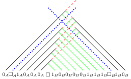
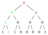
Figure 2: A cellular automaton computing the tree problem, and the corresponding tree

∎

The problem with the previous proof is that we build an artificial and complicated CA, with many states and an unclear local rule. A more accurate question is : Are there elementary CA with a low multi-round communication complexity, but a high lower bound for one-round protocols? We leave this as an open problem.

Considering the recent results by D. Woods and T. Neary [9], a very natural question one could ask is the following: What do computational properties of CA, such as P-completeness, imply on the its communication complexity? As shown by the following proposition, one can build P-complete cellular automata with arbitrarily low communication complexity.

Proposition 3.

For any ${k\geq 1}$, there exists a P-complete CA $\mathcal{A}$ such that ${\mathbf{cc}(\mathcal{A})\in O(n^{1/k})}$.

Proof sketch.

Consider any Turing machine $\mathcal{M}$. We construct a CA $\mathcal{A}$ able to simulate $\mathcal{M}$ only slowly but still in polynomial time: it takes $n^{k}$ steps of $\mathcal{A}$ to simulates $n$ steps of $\mathcal{M}$. Hence, by a suitable choice of $\mathcal{M}$, $\mathcal{A}$ is P-complete.

First it is easy to construct a CA simulating $\mathcal{M}$ in real time. We encode each symbol of the tape alphabet of the Turing machine by a CA state, and add a “layer” for the head, with ’$\rightarrow$’ symbols on its left and ’$\leftarrow$’ symbols on its right. We guarantee this way that there can be only one head : if a ’$\rightarrow$’ state is adjacent to a ’$\leftarrow$’ state without head between them, we propagate an “error” state destroying everything.

We then add a new layer to slow down the simulation: it consists in a single particle (we use the same trick to ensure that there is only one particle) moving left and right inside a marked region of the configuration. More precisely, it goes right until it reaches the end of the marked region, then it adds a marked cell at the end and starts to move left to reach the other end, doing the same thing forever. Clearly, for any cell in a finite marked region, seeing $n$ traversals of the particle takes $\Omega(n^{2})$ steps. Then, the idea is to authorize heads moves in the previous construction only at particle traversals. This way, $n$ steps of $\mathcal{M}$ require $n^{2}$ time steps of the automaton. By adding another layer, one can also slow down the above particle with the same principle and it is not difficult to finally construct a CA $\mathcal{A}$ such that $n$ steps of $\mathcal{M}$ require $n^{k}$ time steps of $\mathcal{A}$.

Now, the communication complexity of $\mathcal{A}$ is $O(n^{1/k})$ because on any input of size $n$, either the “error” appears, or a correct computation of $O(n^{1/k})$ steps of $\mathcal{M}$ occurs. Distinguishing the two cases takes only constant communication. Moreover, in the case of a correct computation, it is sufficient to determine the initial position of particles, the sizes of marked regions (cost $O(\log(n)$), and the initial position of the Turing heads as well as the $O(n^{1/k})$ surrounding states. ∎

3.2 Upper bounds

We propose here a first scheme of complexity classes in cellular automata, based on their communication complexity. What we actually measure is $2^{D(f)}$. This is mainly justified by experiments : the protocols we got for cellular automata with $D(f)=2\log n$ seemed much more sophisticated than those in $\log n$. This is also justified by the fact that what we actually compute is either the number of different rows or columns, or the number of rectangles in the matrices. Thus, in the rest of this article, we will use the terms bounded or constant for CA with communication complexity bounded by a constant, linear for CA with communication complexity $\log n+O(1)$, quadratic for CA with communication complexity $2\log n+O(1)$, and so on.

In this section, we give some well-known properties of CA that induce a bounded communication complexity. The results below are adaptations of ideas of [4] to the formalism adopted in the present paper.

Proposition 4.

Let $\mathcal{A}$ be any CA of local function $f$. If there is a function ${g:\mathbb{N}\rightarrow\mathbb{N}}$ such that $f^{n}$ depends on only $g(n)$ cells, then ${\mathbf{cc}(\mathcal{A})\leq g(n)/2}$.

Following the work of M. Sablik [15], one can characterize the set of CA having a bounded number of dependant cells (i.e. a bounded function $g(n)$): they are exactly these CA which are equicontinuous in some direction (theorem 4.3 of [15]). This set contains the nilpotent CA (a CA is nilpotent if it converges to a unique configuration from any initial configuration, i.e. $f^{n}$ is a constant for any large enough $n$).

Corollary 1.

If $\mathcal{A}$ is equicontinuous in some direction then ${\mathbf{cc_{1}}(\mathcal{A})}$ is bounded.

Another set of CA with that property is the set of linear CA. A CA $\mathcal{A}$ with state set $S$, radius $r$ and local global rule $G$ is linear if there is an operator $\oplus$ such that ${(S,\oplus)}$ is a semi-group with neutral element $e$ and for all configurations $c$ and $c^{\prime}$ we have:

$$G(c\ \overline{\oplus}\ c^{\prime})=G(c)\ \overline{\oplus}\ G(c^{\prime}),$$

where $\overline{\oplus}$ is the uniform extension of $\oplus$ to configurations.

Proposition 5.

If $\mathcal{A}$ is linear then ${\mathbf{cc_{1}}(\mathcal{A})}$ is bounded.

The proof appears in [4] in a different setting. The idea is that there is a simple one-round protocol to compute linear functions: Alice and Bob can each compute on their own the image the function would produce assuming the other party has only the neutral element as input, then Alice or Bob communicate this result to the other who can answer the final result by linearity.

3.3 Simulation and universality

Since the pioneering work of J. von Neumman [10], universality in CA has received a lot of attention (see [13] for a survey). Historically, the notion of universality used for CA was more or less an adaptation of the classical Turing-universality. Later, a stronger notion called intrinsic universality was proposed: a CA is intrinsically universal if it is able to simulate any other CA. This definition relies on a notion of simulation which is formalized below.

The base ingredient is the relation of sub-automaton. A CA $\mathcal{A}$ is a sub-automaton of a CA $\mathcal{B}$, denote ${\mathcal{A}\sqsubseteq\mathcal{B}}$, if there is an injective map $\iota$ from $S_{\mathcal{A}}$ to $S_{\mathcal{B}}$ such that ${\overline{\iota}\circ G_{\mathcal{A}}=G_{\mathcal{B}}\circ\overline{\iota}}$, where ${\overline{\iota}:S_{\mathcal{A}}^{\mathbb{Z}}\rightarrow S_{\mathcal{B}}^{\mathbb{Z}}}$ denotes the uniform extension of $\iota$.

A CA $\mathcal{A}$ simulates a CA $\mathcal{B}$ if some rescaling of $\mathcal{A}$ is a sub-automaton of some rescaling of $\mathcal{B}$. The ingredients of the rescalings are simple: packing cells into blocs, iterating the rule and composing with a translation. Formally, given any state set $Q$ and any $m\geq 1$, we define the bijective packing map ${b_{m}:Q^{\mathbb{Z}}\rightarrow\bigl{(}Q^{m}\bigr{)}^{\mathbb{Z}}}$ by:

$$\forall z\in\mathbb{Z}:\bigl{(}b_{m}(c)\bigr{)}(z)=\bigl{(}c(mz),\ldots,c(mz+m-1)\bigr{)}$$

for all ${c\in Q^{\mathbb{Z}}}$. The rescaling ${\mathcal{A}}^{<m,t,z>}$ of $\mathcal{A}$ by parameters $m$ (packing), ${t\geq 1}$ (iterating) and ${z\in\mathbb{Z}}$ (shifting) is the CA of state set $Q^{m}$ and global rule:

$$b_{m}\circ\sigma_{z}\circ G_{\mathcal{A}}^{t}\circ b^{-1}_{m}.$$

With these definitions, we say that $\mathcal{A}$ simulates $\mathcal{B}$, denoted ${\mathcal{A}\preccurlyeq\mathcal{B}}$, if there are rescaling parameters $m_{1}$, $m_{2}$, $t_{1}$, $t_{2}$, $z_{1}$ and $z_{2}$ such that ${{\mathcal{A}}^{<m_{1},t_{1},z_{1}>}\sqsubseteq{\mathcal{B}}^{<m_{2},t_{2},z_{2}>}}$.

We can now naturally define the notion of universality associated to this simulation relation.

Definition 5.

$\mathcal{A}$ is intrinsically universal if for all $\mathcal{B}$ it holds ${\mathcal{B}\preccurlyeq\mathcal{A}}$.

This definition of universality may seem very resctrictive. In fact, many so-called universal CA (i.e. Turing-universal CA) are also intrinsically universal (see [13] and [3] for the particular case of Game of Life), although there is still a gap for one-dimensional CA (the elementary CA 110 is Turing-universal and no elementary CA is known to be intrinsically universal). Moreover, intrinsic universality appears to be very common in some classes of CA (see [16]).

But, most importantly, by completely formalizing the notion of universality, we facilitate the proof of negative results.

We are going to show that the tool of communication complexity is precisely a good candidate to obtain negative results. The idea is simple: if $\mathcal{A}$ simulates $\mathcal{B}$ then the communication complexity of $\mathcal{A}$ must be ’greater’ than the communication complexity of $\mathcal{B}$.

More precisely, we consider the following relation of comparison between functions from $\mathbb{N}$ to $\mathbb{N}$:

$$\phi_{1}\prec\phi_{2}\iff\exists\alpha,\beta,\gamma\geq 1,\forall n\in\mathbb{N}:\phi_{1}(\alpha n)\leq\beta\phi_{2}(\gamma n).$$

Proposition 6.

If $\mathcal{A}\preccurlyeq\mathcal{B}$ then ${\mathbf{cc}(\mathcal{A})\prec\mathbf{cc}(\mathcal{B})}$.

Proof sketch.

We consider successively each ingredient involved in the simulation relation:

Sub-automaton:

if ${\mathcal{A}\sqsubseteq\mathcal{B}}$ then each valid protocol to compute iterations of $\mathcal{B}$ is also a valid protocol to compute iterations of $\mathcal{A}$ (up to state renaming).

Iterating:

the complexity function of $\mathcal{A}^{t}$ is ${n\mapsto\phi(t\cdot n)}$ if $\phi$ is the complexity function of $\mathcal{A}$.

Shifting:

this operation only affects the splitting of inputs. Since we always take in each case the splitting of maximum complexity, this has no influence on the final complexity function.

Packing:

let $\mathcal{A}$ be CA with local rule $f$ and states set $S$. Consider any sequence of valid protocols $(P_{j})$, one for each splitting of inputs of $f^{n}$, and denote by ${h:(S^{m})^{i}\times(S^{m})^{k-i}\rightarrow S^{m}}$ some splitting of the $n$th iteration of the local rule of ${{\mathcal{A}}^{<m,1,0>}}$. By definition of packing map $b_{m}$, a valid protocol for $h$ is deduced by simultaneous application of protocols ${P_{j},\ldots,P_{j+m-1}}$ (for a suitable choice of $j$), each being used to determined one component of the resulting value of $h$ which belongs to $S^{m}$. It follows that ${\mathbf{cc}(h)\leq m\cdot\mathbf{cc}(f^{n})}$.

Therefore we have: ${\mathbf{cc}(\mathcal{A})\prec\mathbf{cc}\left({\mathcal{A}}^{<m,t,z>}\right)}$, ${\mathbf{cc}\left({\mathcal{A}}^{<m,t,z>}\right)\prec\mathbf{cc}(\mathcal{A})}$ and if ${\mathcal{A}\sqsubseteq\mathcal{B}}$ then ${\mathbf{cc}(\mathcal{A})\prec\mathbf{cc}(\mathcal{B})}$. ∎

From Proposition 1, we derive the following necessary condition for intrinsic universality. It is one of the main motivations to study communication complexity of CA, both theoretically and experimentally.

Corollary 2.

If $\mathcal{A}$ is intrinsically universal then ${\mathbf{cc}(\mathcal{A})\in\Omega(n)}$.

4 The one-round communication complexity of ECA

In this section we concentrate on elementary cellular automata (ECA) : dimension one, two states, and radius $r=1$. And we split the input as follows : $f:\{0,1\}^{n}\times\{0,1\}^{n+1}\rightarrow\{0,1\}$. Since any ECA has the same (one-round) communication complexity as its reflex and its conjugate, we propose here a classification of the 88 nonisomorphic ECA. Since we only consider one-round communication complexity here, Fact 1 allows us to consider matrices associated to functions and study the number of their different rows or columns.

Therefore, for the sake of clarity, the name we give to classes of ECA is related to the number of different rows and columns (instead of the one-round communication complexity, which is the logarithm of the previous).

4.1 Bounded (by a constant)

As shown above, several results allow us to bound the (one-round) communication complexity of many CA.

The ECA proved to be in this class are the following 44 ones: 0, 1, 2, 3, 4, 5, 7, 8, 10, 12, 13, 15, 19, 24, 27, 28, 29, 32, 34, 36, 38, 42, 46, 51, 60, 72, 76, 78, 90, 105, 108, 128, 130, 136, 138, 140, 150, 156, 160, 162, 170, 172, 200, 204 (and all their reflexes, conjugates, and reflex-conjugates).

4.2 Linear

Consider for instance rule 178, which has been studied recently by D. Regnault [14] using percolation theory. The author considered the case where each cell has an independent probability $\rho$ to be updated in each step. He studied Rule 178 because it “exhibited rich behavior such as phase transition”. Despite its complexity, this CA was amenable to formal analysis: the proofs were based on a coupling between its space-time diagram and oriented percolation on a graph.

It is not difficult, using the methods of [8], to prove that the communication complexity of CA 178 grows as $\Theta(n)$. Notice that in order to get such a result we must find, on one hand, a communication protocol (upper bound) of complexity $\approx\log(n)$ and, on the other hand, to exhibit a “fooling set” (i.e. a set $C$ of configurations such that for any couple $(x,y)$ of configurations of $C$, $x$ and $y$ are necessarily in two distinct monochromatic rectangles) of size in $\Omega(n)$.

The ECA Rule 178 is given by the following local rule :

0 0 0 0

1 0 0 1

0 0 1 0

0 0 1 1

1 1 0 0

1 1 0 1

0 1 1 0

1 1 1 1

There is a very simple protocol ${\cal P}$ in $\log n+1$ bits for it: if we call $c$ the value of the central cell at the beginning (Bob knows it), then Bob sends the length of the longest string of cells with value $c$, starting from the left of his part, to Alice.

Proposition 7.

Protocol ${\cal P}$ is correct for ECA Rule 178.

Proof.

First remark that configurations $01$ and $10$ map to each other for any values of their right or left neighbour (which we can see in figure 3 where undetermined cells are represented in gray), and thus stay stable.

Figure 3: Evolution of $01$ and $10$ for rule 178

So once Alice knows where the first $01$ or $10$ occurs, she can assume w.l.g. that the rest of Bob’s part are only zeros (the final result is the same). But then, she also knows the beginning of Bob’s part, so she can compute the final result of Rule 178. ∎

Proposition 8.

Protocol ${\cal P}$ is optimal even as a multi-round protocol.

Proof.

To show this, we use the results of [8] and exhibit a fooling set. Let

$$C=\{(0^{n-2k-1}10^{2k},c^{2k}\overline{c}c^{n-2k})|0\leq 2k\leq n-1,c\in\{0,1\}\}$$

First remark that the result of Rule 178 on configurations of the form

$$0^{n-2k-1}10^{2k}c^{2k}\overline{c}c^{n-2k}$$

is always $n\mod 2$, while for any $i\neq j$, the result of $0^{n-2i-1}10^{2i}c^{2j}\overline{c}c^{n-2j}$ is $n+1\mod 2$.

For the case $c=1$, this is shown by our previous remark on stable configuration. For $c=0$, this is a simple remark on the space-time diagrams of rule 178.

Then $|C|=2\cdot\lfloor n/2\rfloor$, and thus no deterministic protocol, even multiround, could predict rule 178 in less than $\log n+1$ rounds. ∎

Remark.

The same argument can be used for rule 50 (and thus also 179).

We believe that the linearity of Rule 178 and the fact that it is amenable to other types analysis is not a coincidence.

4.3 Quadratic

As soon as we move up in our hierarchy the underlying protocols become rather sophisticated. In fact, for Rule 218, we prove in [5] that if $c=0$ then Alice needs to send 2 positions of her string (2 times $\log(n)$ bits). The difference in the difficulty between sending 1 position ($\Theta(n)$ behavior) and 2 positions ($\Theta(n^{2})$ behavior) is huge.

We encountered Rule 218 when trying to find a (kind of) double-quiescent palindrome-recognizer. Despite the fact that it belongs to class II (according to Wolfram’s classification), it mimics Rule 90 (class III) for very particular initial configurations.

Behind the following “proofs” there are lots of lemmas that we are not even stating. Therefore, the purpose here is just to give an idea of how we proceed. We are considering the case when the central cell is 0. We write $f$ instead of $f_{218}$.

Definition 6.

We say that a word in $\{0,1\}^{*}$ is additive if the 1s are isolated and every consecutive couple of 1s is separated by an odd number of 0s.

Notation 1.

Let $\alpha$ be the maximum index $i$ for which $x_{i}\ldots x_{1}0$ is additive. Let $\beta$ be the maximum index $j$ for which $0y_{1}\ldots y_{j}$ is additive. Let $x^{\prime}=x_{\alpha}\ldots x_{1}\in\{0,1\}^{\alpha}$ and $y^{\prime}=y_{1}\ldots y_{\beta}\in\{0,1\}^{\beta}$.

Notation 2.

Let $l$ be the minimum index $i$ for which $x_{i}=1$. If such index does not exist we define $l=0$. Let $r$ be the minimum index $j$ for which $y_{j}=1$. If such index does not exist we define $r=0$.

Proposition 9.

There exists a one-round $f$-protocol ${\cal P}_{0}$ with cost $2\lceil\log(n)\rceil+1$.

Proof.

Recall the Alice knows $x$ and Bob knows $y$. ${\cal P}_{0}$ goes as follows. Alice sends to Bob $\alpha$, $l$, and $a=f^{\alpha}(x^{\prime},0,0^{\alpha})$. The number of bits is therefore $2\lceil\log(n)\rceil+1$.

If $l=0$ then Bob knows (by definition of $l$) that $x=0^{n}$ and he outputs $f^{n}(0^{n},0,y)$. If $r=0$ his output depends on $\alpha$. If $\alpha=n$ he outputs $a$ and if $\alpha<n$ he outputs 1. We can assume now that neither $l$ nor $r$ are 0. The way Bob proceeds depends mainly on the parity of $|l+r-1|$.

Case $|l+r-1|$ is odd. If $|\alpha-\beta|\geq 1$ Bob outputs 1. If $\alpha=\beta=k$ he outputs $a+f^{k}(0^{k},0,y^{\prime})$.

Case $|l+r-1|$ is even. Bob compares $r$ with $l$. If $l\geq r-1$ then Bob outputs $f^{n}(1^{n-l+1}0^{l-1},0,y)$ if $l\geq r+3$ and 1 otherwise. If $l\leq r-3$ then he outputs $a=f^{\alpha}(x^{\prime},0,0^{\alpha})$ if $r=\alpha+1$ and 1 otherwise. ∎

Now we exhibit lower bounds for the number of different rows of the corresponding matrix. If these bounds appear to be tight then, from Fact 1, they can be used for proving the optimality of our protocol.

Proposition 10.

The cost of any one-round $f$-protocol is at least $2\lceil\log(n)\rceil-5$.

Proof.

Consider the following subsets of $\{0,1\}^{n}$. First, $S_{3}=\{1^{n-3}000\}$. Also,

$$S_{5}=\{1^{n-5}00000,1^{n-5}01000\}.$$

In general, for every $k\geq 2$ such that $2k+1\leq n$, we define

$$S_{2k+1}=\{1^{n-2k-1}0^{2k+1}\}\cup\{1^{n-2k-1}0^{a}10^{b}|\mbox{ $a$ odd, $b$ odd, $b\geq 3$, $a+b=2k$}\}.$$

Let $x_{n}\ldots x_{1}\in S_{2k+1}$ and $\tilde{x}_{n}\ldots\tilde{x}_{1}\in S_{2\tilde{k}+1}$ with $k\neq\tilde{k}$. It follows that the rows of $M_{f}^{c,n}$ indexed by $x_{n}\ldots x_{1}$ and $\tilde{x}_{n}\ldots\tilde{x}_{1}$ are different.

Let $x=x_{n}\ldots x_{1}$, $\tilde{x}=\tilde{x}_{n}\ldots\tilde{x}_{1}\in S_{2k+1}$ with $x\neq\tilde{x}$. It follows that there exists $y=y_{1}\ldots y_{n}\in\{0,1\}^{n}$ such that $f^{n}(x,0,y)\neq f^{n}(\tilde{x},0,y)$. ∎

4.4 Non-polynomial

Our experiments suggested the existence of (at least) two subclasses of this class of “hard” ECA.

• Automata with a high one-round communication complexity but a low matrix rank (suggesting a low multi-round communication complexity), meaning they are easy to predict with several actors and a protocol between them, but the exact influence of each cell of the initial state is hard to determine. We do not know whether this class really exists among ECA, but our experiments suggest that rule 30 may be a candidate.

• Automata that are “intrinsically hard”, meaning that they do not have a deterministic protocol in the previous classes.

5 Conclusion and perspectives

Input splitting. When defining the communication complexity in CA we consider the worst case for splitting the inputs for each $n$. We believe that the sequence ${(s_{n})_{n}}$ of such worst-case splittings is meaningful and raises several interesting questions: Is $s_{n}$ unique for each $n$? If it is the case, what is the function ${n\mapsto s_{n}}$? Is it linear, thus showing a direction of maximal ’information exchange’ along time? What is the meaning of such a direction?

Higher dimensional CA and multi-party protocols. We focused our study on the model where Alice and Bob need to communicate to predict a given CA. There are also other models of protocols with $k$ players, but the difficulty of experimentation would probably not be the same. A greater number of players seems more natural for dimension $2$ or more, since we can partition the set of dependant cells into adjacent regions. But the two-player framework could also be applied to higher dimensional CA.

Nondeterministic protocols. A possible generalization of our definitions of protocols is to allow Alice and Bob to take nondeterministic steps in the protocol tree. This gives us other interesting tools and measures, for instance the notion of a cover of a matrix, which seems linked to circuits. We can find in [8] a link between nondeterministic protocols and the minimal number of rectangles needed to cover a matrix with possible intersections between rectangles.

Probabilistic protocols. Another relevant generalization of communication complexity for the study of CA is randomized complexity, where errors are allowed. In this model, Alice and Bob are allowed to toss a coin before communicating (see [7] regarding one-round randomized complexity and [11] for many-round). Allowing randmoness just changes the notion of complexity and can be applied to deterministic CA, but it may make sense to use this framework for stochastic CA (see for instance [14]).

References

- [1]
- [2] A. Cobham (1964): The intrinsic computational difficulty of functions. In: Congress for Logic, Mathematics and Philosophy of science. pp. 24–30.
- [3] B. Durand & Z. Róka (1999): Cellular Automata: a Parallel Model, Mathematics and its Applications. 460, chapter The game of life:universality revisited., pp. 51–74. Kluwer Academic Publishers.
- [4] Christoph Dürr, Ivan Rapaport & Guillaume Theyssier (2004): Cellular automata and communication complexity. Theor. Comput. Sci. 322(2), pp. 355–368. Available at http://dx.doi.org/10.1016/j.tcs.2004.03.017.
- [5] Eric Goles, Cedric Little & Ivan Rapaport (2008): Understanding a non-trivial cellular automaton by finding its simplest underlying communication protocol. In: Seok-Hee Hong & Hiroshi Nagamochi, editors: ISAAC, Lecture Notes in Computer Science 2380. Springer, p. To appear.
- [6] Juraj Hromkovic & Georg Schnitger (1997): Communication Complexity and Sequential Compuation. In: MFCS ’97: Proceedings of the 22nd International Symposium on Mathematical Foundations of Computer Science. Springer-Verlag, London, UK, pp. 71–84.
- [7] Ilan Kremer, Noam Nisan & Dana Ron (2001): On randomized one-round communication complexity. Computational Complexity 10(4), pp. 314–315.
- [8] Eyal Kushilevitz & Noam Nisan (1997): Communication complexity. Cambridge university press.
- [9] Turlough Neary & Damien Woods (2006): P-completeness of cellular automaton Rule 110. In: In International Colloquium on Automata Languages and Programming (ICALP), volume 4051 of LNCS. Springer, pp. 132–143.
- [10] John von Neumann (1967): The theory of self-reproducing cellular automata. University of Illinois Press, Urbana, Illinois.
- [11] Noam Nisan & Avi Wigderson (1993): Rounds in Communication Complexity Revisited. SIAM J. Comput. 22(1), pp. 211–219.
- [12] Noam Nisan & Avi Wigderson (1994): On Rank vs. Communication Complexity. Electronic Colloquium on Computational Complexity (ECCC) 1(1). Available at http://eccc.hpi-web.de/eccc-reports/1994/TR94-001/index.html.
- [13] Nicolas Ollinger (2008): Universalities in Cellular Automata: a (short) survey. In: B. Durand, editor: Symposium on Cellular Automata Journées Automates Cellulaires (JAC’08). MCCME Publishing House, Moscow, pp. 102–118.
- [14] Damien Regnault (2008): Directed Percolation Arising in Stochastic Cellular Automata Analysis. In: Edward Ochmanski & Jerzy Tyszkiewicz, editors: MFCS, Lecture Notes in Computer Science 5162. Springer, pp. 563–574.
- [15] Mathieu Sablik (2008): Directional dynamics for cellular automata: A sensitivity to initial condition approach. Theor. Comput. Sci. 400(1-3), pp. 1–18.
- [16] Guillaume Theyssier (2005): How Common Can Be Universality for Cellular Automata? In: STACS. pp. 121–132. Available at http://dx.doi.org/10.1007/b106485
- [17] Andrew Chi-Chih Yao (1979): Some Complexity Questions Related to Distributive Computing (Preliminary Report). In: STOC. ACM, pp. 209–213.