Measurements of $D$ Meson Decays to Two Pseudoscalar Mesons

Abstract

Using data collected on the $\psi(3770)$ resonance and near the $D^{\ast\pm}_{s}D^{\mp}_{s}$ peak production energy by the CLEO-c detector, we study the decays of the possible $D\rightarrow PP$ modes and report measurements of or upper limits on all branching fractions for Cabibbo-favored, singly-Cabibbo-suppressed, and doubly-Cabibbo-suppressed $D\rightarrow PP$ decays except modes involving $K^{0}_{L}$ (and except $D^{0}\rightarrow K^{+}\pi^{-}$). We normalize with respect to the Cabibbo-favored $D$ modes, $D^{0}\rightarrow K^{-}\pi^{+}$, $D^{+}\rightarrow K^{-}\pi^{+}\pi^{+}$, and $D^{+}_{s}\rightarrow K^{+}K^{0}_{S}$.

I Introduction

There are many possible exclusive decays of charmed $D$ mesons to a pair of mesons from the lowest-lying pseudoscalar meson nonet. The decay can be to any pair of $K^{+}$, $K^{-}$, $\pi^{+}$, $\pi^{-}$, $\eta$, $\eta^{\prime}$, $\pi^{0}$, $K^{0}$, or $\bar{K^{0}}$, with total charge 0 or $\pm 1$. Measurements of the complete set of decays can be used to test flavor topology and SU(3) predictions and to specify strong phases of decay amplitudes through triangle relations RosnerPaper . Moreover, many $CP$ asymmetries (expected to be less than ${\cal O}(10^{-3})$ in the Standard Model) can be studied. The detectable neutral kaons are $K^{0}_{S}$ and $K^{0}_{L}$, not $K^{0}$ and $\bar{K^{0}}$, so the observable decays are $XK^{0}_{S}$ and $XK^{0}_{L}$. In this study, we consider only $K^{0}_{S}$, not $K^{0}_{L}$, and report all branching fractions for Cabibbo-favored, singly-Cabibbo-suppressed, and doubly-Cabibbo-suppressed $D\rightarrow PP$ decays except modes involving $K^{0}_{L}$ and except the doubly-Cabibbo-suppressed decay $D^{0}\rightarrow K^{+}\pi^{-}$. We normalize with respect to the Cabibbo-favored $D$ modes, $D^{0}\rightarrow K^{-}\pi^{+}$ CLEO:sys , $D^{+}\rightarrow K^{-}\pi^{+}\pi^{+}$ CLEO:sys , and $D^{+}_{s}\rightarrow K^{+}K^{0}_{S}$ Peterpaper . (More precisely, we normalize the $D^{0}\rightarrow PP$ decays with respect to the sum of the Cabibbo-favored mode $D^{0}\rightarrow K^{-}\pi^{+}$ and the doubly-Cabibbo-suppressed mode $D^{0}\rightarrow K^{+}\pi^{-}$. The latter is 0.4% of the former.)

II The detector

Data for this analysis were taken at the Cornell Electron Storage Ring (CESR) using the CLEO-c general-purpose solenoidal detector, which is described in detail elsewhere Briere:2001rn ; Kubota:1991ww ; cleoiiidr ; cleorich . The charged particle tracking system covers a solid angle of 93% of $4\pi$ and consists of a small-radius, six-layer, low-mass, stereo wire drift chamber, concentric with, and surrounded by, a 47-layer cylindrical central drift chamber. The chambers operate in a 1.0 T magnetic field. The root-mean-square (rms) momentum resolution achieved with the tracking system is approximately 0.6% at $p=1$ GeV/$c$ for tracks that traverse all layers of the drift chamber. Photons are detected in an electromagnetic calorimeter consisting of 7800 cesium iodide crystals and covering 95% of $4\pi$, which achieves a photon energy resolution of 2.2% at $E_{\gamma}=1$ GeV and 6% at 100 MeV. We utilize two particle identification (PID) devices to separate charged kaons from pions: the central drift chamber, which provides measurements of ionization energy loss ($dE/dx$), and, surrounding this drift chamber, a cylindrical ring-imaging Cherenkov (RICH) detector, whose active solid angle is 80% of $4\pi$. The combined PID system has a pion or kaon efficiency $>85\%$ and a probability of pions faking kaons (or vice versa) $<5\%$ CLEO:sys . The response of the CLEO-c detector is studied with a detailed GEANT-based geant Monte Carlo (MC) simulation, with initial particle trajectories generated by EvtGen evtgen and final state radiation produced by PHOTOS photos . Simulated events are reconstructed and selected for analysis with the reconstruction programs and selection criteria used for data.

III The Data Sample

For $D^{0}$ and $D^{+}$ meson decays, we utilize a total integrated luminosity of 818 $\mathrm{pb}^{-1}$ of $e^{+}e^{-}$ data collected at center-of-mass (CM) energies near $E_{\text{cm}}=3774$ MeV. The data sample contains about $2.4\times 10^{6}$ $D^{+}D^{-}$ events (events of interest), three million $D^{0}\bar{D^{0}}$ events (events of interest), fifteen million $e^{+}e^{-}\rightarrow u\bar{u},\ d\bar{d},$ or $s\bar{s}$ continuum events, three million $e^{+}e^{-}\rightarrow\tau^{+}\tau^{-}$ events, and three million $e^{+}e^{-}\rightarrow\gamma\psi^{\prime}$ radiative return events (sources of background), as well as Bhabha events, $\mu$-pair events, and $\gamma\gamma$ events (useful for luminosity determination and resolution studies). For the $D_{s}^{+}$ meson decays, we use a data sample of $e^{+}e^{-}\rightarrow D^{\ast\pm}_{s}D^{\mp}_{s}$ events collected at the CM energy 4170 MeV, near $D^{\ast\pm}_{s}D^{\mp}_{s}$ peak production of $\sim$1 nb Poling:2006da . The data sample consists of an integrated luminosity of 586 $\mathrm{pb}^{-1}$ containing about $5.4\times 10^{5}$ $D^{\ast\pm}_{s}D^{\mp}_{s}$ pairs. Other charm production totals $\sim$7 nb Poling:2006da , and the underlying light-quark “continuum” is about 12 nb. Through this paper, charge conjugate modes are implicitly assumed, unless otherwise noted.

IV Procedure

IV.1 $D^{0}$ and $D^{+}$

Here we employ a single-tag (ST) technique extensively used by CLEO-c CLEO:sys ; Peterpaper ; FanKpi0 ; FanDspp , pioneered by the Mark III Collaboration at SPEAR for measuring $D^{0}$ and $D^{+}$ branching fractions mark3a ; mark3b , which exploits a feature of near-threshold production of charmed mesons, i.e. $M_{\mathrm{bc}}$ and $\Delta E$, see below.

We formed $D$ and $\bar{D}$ candidates in all $D\rightarrow PP$ decay modes from combinations of $\pi^{\pm}$, $K^{\pm}$, $\pi^{0}$, $K^{0}_{S}$, $\eta$, and $\eta^{\prime}$ candidates selected using the standardized requirements which are common to many CLEO-c analyses involving $D$ decays. The $\psi$(3770) resonance is below the kinematic threshold for $D\bar{D}\pi$ production, so the events of interest, $e^{+}e^{-}\rightarrow\psi(3770)\rightarrow D\bar{D}$, have $D$ mesons with energy equal to the beam energy. Two variables reflecting energy and momentum conservation are used to identify valid $D$ candidates. They are $\Delta E\equiv\sum_{i}E_{i}-E_{\rm beam}$, and $M_{\mathrm{bc}}\equiv\sqrt{E^{2}_{\rm beam}-(\sum_{i}\mathbf{p}_{i})^{2}}$, where $E_{i},\ \mathbf{p}_{i}$ are the energy and momentum of the decay products of a $D$ candidate. For a correct combination of particles, $\Delta E$ will be consistent with zero, and the beam-constrained mass $M_{\mathrm{bc}}$ will be consistent with the $D$ mass. Candidates are rejected if they fail mode-dependent $\Delta E$ requirements. If there is more than one candidate in a particular $D$ or $\bar{D}$ decay mode, we choose the candidate with the smallest $|\Delta E|$.

IV.2 $D^{+}_{s}$

Unlike $D\bar{D}$ threshold events, conventional $\Delta E$ and $M_{\text{bc}}$ variables are no longer good variables for $D_{s}$ from $D_{s}^{\ast+}D_{s}^{-}$ decays, as the $D_{s}$ can either be a primary or secondary (from a $D^{\ast}_{s}$ decay), with different momentum. We use the reconstructed invariant mass of the $D_{s}$ candidate, $M(D_{s})$, and the mass recoiling against the $D_{s}$ candidate, $M_{\text{recoil}}(D_{s})\equiv\sqrt{(E_{0}-E_{D_{s}})^{2}-(\mathbf{p}_{0}-\mathbf{p}_{D_{s}})^{2}}$, as our primary kinematic variables to select a $D_{s}$ candidate. Here $(E_{0},\mathbf{p}_{0})$ is the net four-momentum of the $e^{+}e^{-}$ system, taking the finite beam crossing angle into account, $\mathbf{p}_{D_{s}}$ is the momentum of the $D_{s}$ candidate, $E_{D_{s}}=\sqrt{m^{2}_{D_{s}}+\mathbf{p}^{2}_{D_{s}}}$, and $m_{D_{s}}$ is the known $D_{s}$ mass PDGValue . We make no requirements on the decay of the other $D_{s}$ in the event.

There are two components in the recoil mass distribution, a peak around the $D^{\ast}_{s}$ mass if the candidate is due to the primary $D_{s}$ and a rectangular shaped distribution if the candidate is due to the secondary $D_{s}$ from a $D^{\ast}_{s}$ decay. The edges of $M_{\text{recoil}}(D_{s})$ from the secondary $D_{s}$ are kinematically determined (as a function of $\sqrt{s}$ and known masses), and at $\sqrt{s}=4170$ MeV, $\Delta M_{\text{recoil}}(D_{s})\equiv M_{\text{recoil}}(D_{s})-m_{D^{\ast}_{s}}$ is in the range $[-54,57]$ MeV. Initial state radiation causes a tail on the high side, above 57 MeV. We select $D_{s}$ candidates within the $-55~{}\text{MeV}\leq\Delta M_{\text{recoil}}(D_{s})<+55~{}\text{MeV}$ range. This window allows both primary and secondary $D_{s}$ candidates to be selected.

We also require a photon consistent with coming from $D^{\ast+}_{s}\rightarrow D^{+}_{s}\gamma$ decay, by looking at the mass recoiling against the $D_{s}$ candidate plus $\gamma$ system, $M_{\text{recoil}}(D_{s}\gamma)\equiv\sqrt{(E_{0}-E_{D_{s}}-E_{\gamma})^{2}-(\mathbf{p}_{0}-\mathbf{p}_{D_{s}}-\mathbf{p}_{\gamma})^{2}}$. For correct combinations, this recoil mass peaks at $m_{D_{s}}$, regardless of whether the candidate is due to a primary or a secondary $D_{s}$. We require $|M_{\text{recoil}}(D_{s}\gamma)-m_{D_{s}}|<30~{}\text{MeV}$. This requirement improves the signal to noise ratio, important for the suppressed modes. Every event is allowed to contribute a maximum of one $D_{s}$ candidate per mode and charge. If there are multiple candidates, the one with $M_{\text{recoil}}(D_{s}\gamma)$ closest to $m_{D_{s}}$ is chosen.

IV.3 Common

Our standard final-state particle selection requirements are described in detail elsewhere CLEO:sys . Charged tracks produced in the $D$ decay are required to satisfy criteria based on the track fit quality, and angles $\theta$ with respect to the beam line, satisfying $|\cos\theta|<0.93$. Momenta of charged particles utilized in $D^{0}$ and $D^{+}$ candidate reconstructions must be above 50 MeV/$c$, while those for $D_{s}$ must be above 100 MeV/$c$ to eliminate the soft pions from $D^{\ast}\bar{D}^{\ast}$ and $D^{\ast}\bar{D}$ decays (through $D^{\ast}\to\pi D$). Tracks must also be consistent with their coming from the interaction point in three dimensions. Pion and kaon candidates are required to have $dE/dx$ measurements within three standard deviations ($3\sigma$) of the expected value. For tracks with momenta greater than 700 MeV/$c$, RICH information, if available, is combined with $dE/dx$.

The $K^{0}_{S}$ candidates are selected from pairs of oppositely-charged and vertex-constrained tracks having invariant mass within 7.5 MeV, or roughly 3$\sigma$, of the known $K^{0}_{S}$ mass PDGValue . We identify $\pi^{0}$ candidates via $\pi^{0}\rightarrow\gamma\gamma$, detecting the photons in the CsI calorimeter. To avoid having both photons in a region of poorer energy resolution, we require that at least one of the photons be in the “good barrel” region, $|\cos\theta_{\gamma}|<0.80$. We require that a calorimeter cluster has a measured energy above 30 MeV, has a lateral distribution consistent with that from photons, and not be matched to any charged track. The invariant mass of the photon pair is required to be within 3$\sigma$ ($\sigma\sim$ 6 MeV) of the known $\pi^{0}$ mass. A $\pi^{0}$ mass constraint is imposed when $\pi^{0}$ candidates are used in further reconstruction. We reconstruct $\eta$ candidates in the decay of $\eta\rightarrow\gamma\gamma$. Candidates are formed using a similar procedure as for $\pi^{0}$ except that $\sigma\sim$ 12 MeV. We reconstruct $\eta^{\prime}$ candidates in the decay mode $\eta^{\prime}\rightarrow\pi^{+}\pi^{-}\eta$. We require $|m_{\pi^{+}\pi^{-}\eta}-m_{\eta^{\prime}}|<10$ MeV.

V Results

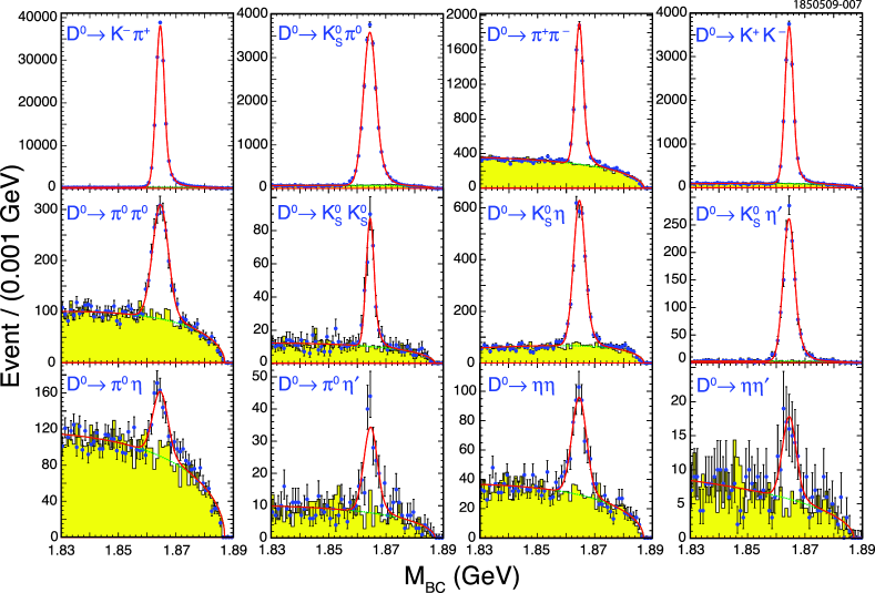
Figure 1: $M_{\mathrm{bc}}$ distributions of $D^{0}$ modes. For each distribution, the points are obtained from the $\Delta E$ signal region, the shaded histogram is from the $\Delta E$ sidebands, and the line is the fit.

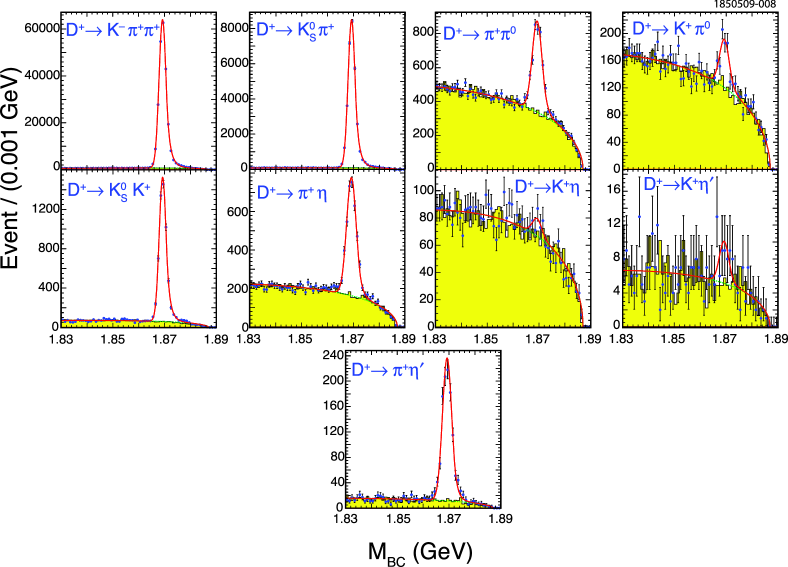
Figure 2: $M_{\mathrm{bc}}$ distributions of $D^{+}$ modes. For each distribution, the points are obtained from the $\Delta E$ signal region, the shaded histogram is from the $\Delta E$ sidebands, and the line is the fit.

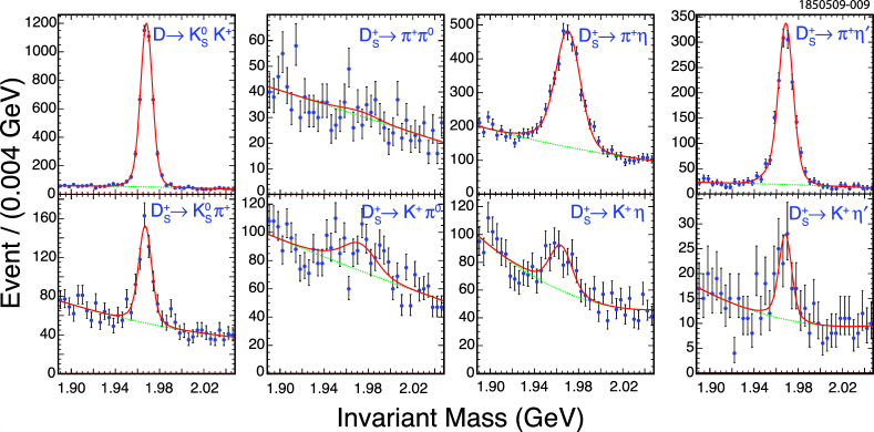
Figure 3: $M(D_{s})$ distributions for $D_{s}$ modes. For each distribution, the points are the data and the superimposed line is the fit (the dotted line is the fitted background). The distribution for $D_{s}^{+}\rightarrow\pi^{+}\pi^{0}$ has tighter requirements than the other modes – see text.

V.1 $D^{0}$ and $D^{+}$

The $M_{\mathrm{bc}}$ distributions for the $D^{0}$ and $D^{+}$ candidate combinations are shown in Figs. 1 and 2, respectively. The points show the data and the lines are fits. The normalization modes $D^{0}\rightarrow K^{-}\pi^{+}$ and $D^{+}\rightarrow K^{-}\pi^{+}\pi^{+}$ are essentially background-free. The backgrounds of all modes are well described by the distributions obtained from the $\Delta E$ sidebands. We perform a binned maximum likelihood fit to extract the $D^{0}$ or $D^{+}$ signal yield from each $M_{\mathrm{bc}}$ distribution. For the signal, we use an inverted Crystal Ball line shape CBFunc , which is a Gaussian with a high-side tail. For the background, we use an ARGUS function ArgusFunc , with the shape parameter determined from the $\Delta E$ sideband $M_{\mathrm{bc}}$ distribution, the high-end cutoff given by $E_{\rm{beam}}$, and the normalization determined from the fit to the $\Delta E$ signal region. Results of the fits are shown in Table 1. Table 1 also includes the detection efficiency for each mode. The efficiencies include sub-mode branching fractions PDGValue and have been corrected to include four known small differences between data and Monte Carlo simulation, in particular $\pi^{0}$-finding efficiency 0.96, $\eta$-finding efficiency 0.935, $\pi^{\pm}$ particle identification 0.995, and $K^{\pm}$ particle identification 0.99, data efficiency being smaller than MC efficiency by those ratios.

V.2 $D^{+}_{s}$

The resulting $M(D_{s})$ distributions for $D_{s}$ modes are shown in Fig. 3. The points show the data and the lines are fits. We perform binned maximum likelihood fits to extract signal yields from the $M(D_{s})$ distributions. For the signal, we use the sum of two Gaussians for the line shape. For the background, we use a second-degree polynomial function. Results of the fits and detection efficiencies are given in Table 1.

Table 1: Observed yields from data and reconstruction efficiencies and their statistical uncertainties. The efficiencies include sub-mode branching fractions PDGValue and have been corrected to include several known small differences between data and Monte Carlo simulation.

Mode	Efficiency (%)	Yield
$D^{0}\rightarrow K^{+}K^{-}$	57.35 $\pm$ 0.16	13782 $\pm$ 136
$D^{0}\rightarrow K^{0}_{S}K^{0}_{S}$	22.73 $\pm$ 0.13	215 $\pm$ 23
$D^{0}\rightarrow\pi^{+}\pi^{-}$	72.68 $\pm$ 0.14	6210 $\pm$ 93
$D^{0}\rightarrow\pi^{0}\pi^{0}$	32.95 $\pm$ 0.14	1567 $\pm$ 54
$D^{0}\rightarrow K^{-}\pi^{+}$	65.11 $\pm$ 0.15	150259 $\pm$ 420
$D^{0}\rightarrow K^{0}_{S}\pi^{0}$	28.57 $\pm$ 0.14	20045 $\pm$ 165
$D^{0}\rightarrow K^{0}_{S}\eta$	10.08 $\pm$ 0.05	2864 $\pm$ 65
$D^{0}\rightarrow\pi^{0}\eta$	11.97 $\pm$ 0.05	481 $\pm$ 40
$D^{0}\rightarrow K^{0}_{S}\eta^{\prime}$	2.35 $\pm$ 0.02	1321 $\pm$ 42
$D^{0}\rightarrow\pi^{0}\eta^{\prime}$	2.97 $\pm$ 0.02	159 $\pm$ 19
$D^{0}\rightarrow\eta\eta$	4.35 $\pm$ 0.02	430 $\pm$ 29
$D^{0}\rightarrow\eta\eta^{\prime}$	1.06 $\pm$ 0.01	66 $\pm$ 15
$D^{+}\rightarrow K^{-}\pi^{+}\pi^{+}$	54.92 $\pm$ 0.16	231058 $\pm$ 515
$D^{+}\rightarrow K^{0}_{S}K^{+}$	36.62 $\pm$ 0.15	5161 $\pm$ 86
$D^{+}\rightarrow\pi^{+}\pi^{0}$	48.69 $\pm$ 0.15	2649 $\pm$ 76
$D^{+}\rightarrow K^{0}_{S}\pi^{+}$	42.54 $\pm$ 0.16	30095 $\pm$ 191
$D^{+}\rightarrow K^{+}\pi^{0}$	43.29 $\pm$ 0.15	343 $\pm$ 37
$D^{+}\rightarrow K^{+}\eta$	15.95 $\pm$ 0.06	60 $\pm$ 24
$D^{+}\rightarrow\pi^{+}\eta$	18.07 $\pm$ 0.06	2940 $\pm$ 68
$D^{+}\rightarrow K^{+}\eta^{\prime}$	4.29 $\pm$ 0.02	23 $\pm$ 18
$D^{+}\rightarrow\pi^{+}\eta^{\prime}$	4.81 $\pm$ 0.02	1037 $\pm$ 35
$D_{s}^{+}\rightarrow K^{0}_{S}K^{+}$	24.73 $\pm$ 0.14	4076 $\pm$ 71
$D_{s}^{+}\rightarrow\pi^{+}\pi^{0}$	16.60 $\pm$ 0.12	19 $\pm$ 28
$D_{s}^{+}\rightarrow K^{0}_{S}\pi^{+}$	28.15 $\pm$ 0.14	393 $\pm$ 33
$D_{s}^{+}\rightarrow K^{+}\pi^{0}$	29.57 $\pm$ 0.14	202 $\pm$ 70
$D_{s}^{+}\rightarrow K^{+}\eta$	11.40 $\pm$ 0.05	222 $\pm$ 41
$D_{s}^{+}\rightarrow\pi^{+}\eta$	12.70 $\pm$ 0.06	2587 $\pm$ 89
$D_{s}^{+}\rightarrow K^{+}\eta^{\prime}$	2.87 $\pm$ 0.02	56 $\pm$ 17
$D_{s}^{+}\rightarrow\pi^{+}\eta^{\prime}$	3.28 $\pm$ 0.02	1436 $\pm$ 47

V.3 Upper Limits

For most of the $D\rightarrow PP$ modes, very clear signals are found in data. We find no significant evidence for $D^{+}\rightarrow K^{+}\eta$, $D^{+}\rightarrow K^{+}\eta^{\prime}$, and $D_{s}^{+}\rightarrow\pi^{+}\pi^{0}$ decays, and therefore set upper limits on their branching fractions. The $M_{\mathrm{bc}}$ distributions of $D^{+}\rightarrow K^{+}\eta$ and $D^{+}\rightarrow K^{+}\eta^{\prime}$ modes are shown in Fig. 2. Monte Carlo studies indicate that tightening the requirements on $M_{\text{recoil}}(D_{s})$ to $\pm 10$ MeV and $M_{\text{recoil}}(D_{s}\gamma)$ to $\pm 20$ MeV should improve the upper limit on $D^{+}_{s}\rightarrow\pi^{+}\pi^{0}$ decay. Consequently, for $D^{+}_{s}\rightarrow\pi^{+}\pi^{0}$ (and only $D^{+}_{s}\rightarrow\pi^{+}\pi^{0}$), we have applied these tighter requirements. The invariant mass distribution for $D^{+}_{s}\rightarrow\pi^{+}\pi^{0}$ shown in Fig. 3 and the efficiency given in Table 1 have these tighter requirements.

V.4 Background from Non-resonant Decays

Non-resonant $D$ decays can enter into our signal modes with the same final particles. For example, non-resonant $D^{+}\rightarrow\pi^{+}(\pi^{+}\pi^{-})$ can appear in the $D^{+}\rightarrow\pi^{+}K^{0}_{S},K^{0}_{S}\rightarrow\pi^{+}\pi^{-}$ mode. Also, non-resonant $D^{+}\rightarrow\pi^{+}(\pi^{+}\pi^{-}\eta)$ can appear in the $D^{+}\rightarrow\pi^{+}\eta^{\prime},\eta^{\prime}\rightarrow\pi^{+}\pi^{-}\eta$ mode. To understand the backgrounds from non-resonant $D^{0}$ or $D^{+}$ decays, we look at $M_{\mathrm{bc}}$ distributions in the invariant mass sideband regions of the intermediate resonances ($K^{0}_{S}$ or $\eta^{\prime}$). For $D^{+}_{s}$ decays, we follow the same procedure, replacing $M_{\mathrm{bc}}$ with $M(D_{s})$. The scaling factor, from sideband to signal region, is taken to be unity, as indicated by Monte Carlo studies.

For the $D^{0}\rightarrow K^{0}_{S}K^{0}_{S}$ (or $D^{0}\rightarrow K^{0}_{S}\eta^{\prime}$) mode, the scatter plot of $K^{0}_{S}$ candidate invariant mass against the other $K^{0}_{S}$ (or $\eta^{\prime}$) candidate invariant mass is used to define a signal region and two kinds of sideband regions to remove the non-resonant decay background. Again, the scaling factor, from sideband to signal region, is taken to be unity.

V.5 Systematic Uncertainties

We have considered several sources of systematic uncertainty. Some are correlated among different decay modes. These include:

1. the uncertainty associated with the efficiency for finding a track - 0.3% per track CLEO:sys ;

2. an additional 0.6% per kaon track is added CLEO:sys , uncorrelated with item 1;

3. the uncertainty in charged pion identification is 0.3% per $\pi^{\pm}$ CLEO:sys ;

4. the uncertainty in charged kaon identification is 0.3% per $K^{\pm}$ CLEO:sys , uncorrelated with item 3;

5. the relative systematic uncertainties for $\pi^{0}$, $K^{0}_{S}$, and $\eta$ finding efficiencies are 2.0%, 1.8% CLEO:sys , and 4.0%, independent of one another, and independent of the first four-mentioned uncertainties;

6. finally, among the correlated systematic uncertainties, there are the uncertainties in the input branching fractions of the normalization modes, 2.0% for $D^{0}\rightarrow K^{-}\pi^{+}$ CLEO:sys , 2.2% for $D^{+}\rightarrow K^{-}\pi^{+}\pi^{+}$ CLEO:sys , and 5.8% for $D_{s}^{+}\rightarrow K^{0}_{S}K^{+}$ Peterpaper .

Note that for $K^{0}_{S}$, with $K^{0}_{S}\rightarrow\pi^{+}\pi^{-}$, item 1 applies, as the tracks must be found, but item 3 does not apply, as pion identification is not required for $K^{0}_{S}\rightarrow\pi^{+}\pi^{-}$.

The systematic uncertainties that are uncorrelated among the decay modes include those due to choice of signal shape and background shape. They range from $\pm 0.05\%$ for the cleaner decay modes to $\pm 4.55\%$ for the modes with substantial background.

In the Table 2 we separately list, for each decay mode, the quadratic sum of the systematic errors excluding that from the normalization mode, and the error from the uncertainty in the normalization mode.

V.6 $CP$ Asymmetries

The Standard Model predicts that direct $CP$ violation in $D$ decays, e.g., a difference in the branching fractions for $D^{+}_{s}\rightarrow K^{+}\eta$ and $D^{-}_{s}\rightarrow K^{-}\eta$, will be vanishingly small. We have separate yields and efficiencies for $D$ and $\bar{D}$ events, so it is possible to compute asymmetries $\mathcal{A}_{CP}\equiv(\mathcal{B}_{+}-\mathcal{B}_{-})/(\mathcal{B}_{+}+\mathcal{B}_{-})$, which are sensitive to direct $CP$ violation in $D$ decays. All systematic uncertainties cancel in this ratio, with the exception of charged pion and kaon tracking and particle identification efficiencies. Here the relative factor is the charge dependence of the efficiencies in data and Monte Carlo simulations CLEO:sys .

For $D^{0}$ vs. $\bar{D^{0}}$, the only asymmetry we can measure is $K^{-}\pi^{+}$ vs. $K^{+}\pi^{-}$. That difference will contain a component from the difference in the doubly-Cabibbo-suppressed decays $D^{0}\rightarrow K^{+}\pi^{-}$ vs. $\bar{D^{0}}\rightarrow K^{-}\pi^{+}$, as well as the component from the favored decays $D^{0}\rightarrow K^{-}\pi^{+}$ vs. $\bar{D^{0}}\rightarrow K^{+}\pi^{-}$. Our measurement does not separate these two possible asymmetries.

VI Summary

The obtained branching ratios, branching fractions, and $CP$ asymmetries for all $D\rightarrow PP$ modes are shown in Table 2. The values we obtained are consistent with the world averages PDGValue and for the suppressed modes, of better accuracy. No significant $CP$ asymmetries are observed.

Table 2: Ratios of branching fractions to the corresponding normalization modes $D^{0}\rightarrow K^{-}\pi^{+}$, $D^{+}\rightarrow K^{-}\pi^{+}\pi^{+}$, and $D_{s}^{+}\rightarrow K^{0}_{S}K^{+}$; branching fractions results from this analysis; and charge asymmetries $\mathcal{A}_{CP}$. Uncertainties are statistical error, systematic error, and the error from the input branching fractions of normalization modes. (For $D^{0}$, the normalization mode is the sum of $D^{0}\rightarrow K^{-}\pi^{+}$ and $D^{0}\rightarrow K^{+}\pi^{-}$ – see text.)

Mode	$\mathcal{B}_{\text{mode}}/\mathcal{B}_{\text{Normalization}}$ (%)	This result $\mathcal{B}$ (%)	$\mathcal{A}_{CP}$ (%)
$D^{0}\rightarrow K^{+}K^{-}$	10.41 $\pm$ 0.11 $\pm$ 0.11	0.407 $\pm$ 0.004 $\pm$ 0.004 $\pm$ 0.008
$D^{0}\rightarrow K^{0}_{S}K^{0}_{S}$	0.41 $\pm$ 0.04 $\pm$ 0.02	0.0160 $\pm$ 0.0017 $\pm$ 0.0008 $\pm$ 0.0003
$D^{0}\rightarrow\pi^{+}\pi^{-}$	3.70 $\pm$ 0.06 $\pm$ 0.09	0.145 $\pm$ 0.002 $\pm$ 0.004 $\pm$ 0.003
$D^{0}\rightarrow\pi^{0}\pi^{0}$	2.06 $\pm$ 0.07 $\pm$ 0.10	0.081 $\pm$ 0.003 $\pm$ 0.004 $\pm$ 0.002
$D^{0}\rightarrow K^{-}\pi^{+}$	100	3.9058 external input CLEO:sys	0.5 $\pm$ 0.4 $\pm$ 0.9
$D^{0}\rightarrow K^{0}_{S}\pi^{0}$	30.4 $\pm$ 0.3 $\pm$ 0.9	1.19 $\pm$ 0.01 $\pm$ 0.04 $\pm$ 0.02
$D^{0}\rightarrow K^{0}_{S}\eta$	12.3 $\pm$ 0.3 $\pm$ 0.7	0.481 $\pm$ 0.011 $\pm$ 0.026 $\pm$ 0.010
$D^{0}\rightarrow\pi^{0}\eta$	1.74 $\pm$ 0.15 $\pm$ 0.11	0.068 $\pm$ 0.006 $\pm$ 0.004 $\pm$ 0.001
$D^{0}\rightarrow K^{0}_{S}\eta^{\prime}$	24.3 $\pm$ 0.8 $\pm$ 1.1	0.95 $\pm$ 0.03 $\pm$ 0.04 $\pm$ 0.02
$D^{0}\rightarrow\pi^{0}\eta^{\prime}$	2.3 $\pm$ 0.3 $\pm$ 0.2	0.091 $\pm$ 0.011 $\pm$ 0.006 $\pm$ 0.002
$D^{0}\rightarrow\eta\eta$	4.3 $\pm$ 0.3 $\pm$ 0.4	0.167 $\pm$ 0.011 $\pm$ 0.014 $\pm$ 0.003
$D^{0}\rightarrow\eta\eta^{\prime}$	2.7 $\pm$ 0.6 $\pm$ 0.3	0.105 $\pm$ 0.024 $\pm$ 0.010 $\pm$ 0.002
$D^{+}\rightarrow K^{-}\pi^{+}\pi^{+}$	100	9.1400 external input CLEO:sys	-0.1 $\pm$ 0.4 $\pm$ 0.9
$D^{+}\rightarrow K^{0}_{S}K^{+}$	3.35 $\pm$ 0.06 $\pm$ 0.07	0.306 $\pm$ 0.005 $\pm$ 0.007 $\pm$ 0.007	-0.2 $\pm$ 1.5 $\pm$ 0.9
$D^{+}\rightarrow\pi^{+}\pi^{0}$	1.29 $\pm$ 0.04 $\pm$ 0.05	0.118 $\pm$ 0.003 $\pm$ 0.005 $\pm$ 0.003	2.9 $\pm$ 2.9 $\pm$ 0.3
$D^{+}\rightarrow K^{0}_{S}\pi^{+}$	16.82 $\pm$ 0.12 $\pm$ 0.37	1.537 $\pm$ 0.011 $\pm$ 0.034 $\pm$ 0.033	-1.3 $\pm$ 0.7 $\pm$ 0.3
$D^{+}\rightarrow K^{+}\pi^{0}$	0.19 $\pm$ 0.02 $\pm$ 0.01	0.0172 $\pm$ 0.0018 $\pm$ 0.0006 $\pm$ 0.0004	-3.5 $\pm$ 10.7 $\pm$ 0.9
$D^{+}\rightarrow K^{+}\eta$	$<0.14$ (90% C.L.)	$<0.013$ (90% C.L.)
$D^{+}\rightarrow\pi^{+}\eta$	3.87 $\pm$ 0.09 $\pm$ 0.19	0.354 $\pm$ 0.008 $\pm$ 0.018 $\pm$ 0.008	-2.0 $\pm$ 2.3 $\pm$ 0.3
$D^{+}\rightarrow K^{+}\eta^{\prime}$	$<0.20$ (90% C.L.)	$<0.018$ (90% C.L.)
$D^{+}\rightarrow\pi^{+}\eta^{\prime}$	5.12 $\pm$ 0.17 $\pm$ 0.25	0.468 $\pm$ 0.016 $\pm$ 0.023 $\pm$ 0.010	-4.0 $\pm$ 3.4 $\pm$ 0.3
$D_{s}^{+}\rightarrow K^{0}_{S}K^{+}$	100	1.4900 external input Peterpaper	4.7 $\pm$ 1.8 $\pm$ 0.9
$D_{s}^{+}\rightarrow\pi^{+}\pi^{0}$	$<2.3$ (90% C.L.)	$<0.037$ (90% C.L.)
$D_{s}^{+}\rightarrow K^{0}_{S}\pi^{+}$	8.5 $\pm$ 0.7 $\pm$ 0.2	0.126 $\pm$ 0.011 $\pm$ 0.003 $\pm$ 0.007	16.3 $\pm$ 7.3 $\pm$ 0.3
$D_{s}^{+}\rightarrow K^{+}\pi^{0}$	4.2 $\pm$ 1.4 $\pm$ 0.2	0.062 $\pm$ 0.022 $\pm$ 0.004 $\pm$ 0.004	-26.6 $\pm$ 23.8 $\pm$ 0.9
$D_{s}^{+}\rightarrow K^{+}\eta$	11.8 $\pm$ 2.2 $\pm$ 0.6	0.176 $\pm$ 0.033 $\pm$ 0.009 $\pm$ 0.010	9.3 $\pm$ 15.2 $\pm$ 0.9
$D_{s}^{+}\rightarrow\pi^{+}\eta$	123.6 $\pm$ 4.3 $\pm$ 6.2	1.84 $\pm$ 0.06 $\pm$ 0.09 $\pm$ 0.11	-4.6 $\pm$ 2.9 $\pm$ 0.3
$D_{s}^{+}\rightarrow K^{+}\eta^{\prime}$	11.8 $\pm$ 3.6 $\pm$ 0.6	0.18 $\pm$ 0.05 $\pm$ 0.01 $\pm$ 0.01	6.0 $\pm$ 18.9 $\pm$ 0.9
$D_{s}^{+}\rightarrow\pi^{+}\eta^{\prime}$	265.4 $\pm$ 8.8 $\pm$ 13.9	3.95 $\pm$ 0.13 $\pm$ 0.21 $\pm$ 0.23	-6.1 $\pm$ 3.0 $\pm$ 0.3

VII Acknowledgements

We gratefully acknowledge the effort of the CESR staff in providing us with excellent luminosity and running conditions. D. Cronin-Hennessy and A. Ryd thank the A.P. Sloan Foundation. This work was supported by the National Science Foundation, the U.S. Department of Energy, the Natural Sciences and Engineering Research Council of Canada, and the U.K. Science and Technology Facilities Council.

References

- (1) B. Bhattacharya and J. L. Rosner, Phys. Rev. D 77, 114020 (2008).
- (2) S. Dobbs . (CLEO Collaboration), Phys. Rev. D 76, 112001 (2007).
- (3) J. P. Alexander . (CLEO Collaboration), Phys. Rev. Lett. 100, 161804 (2008).
- (4) R. A. Briere et al. (CESR-c and CLEO-c Taskforces, CLEO-c Collaboration), Cornell University, LEPP Report No. CLNS 01/1742 (2001) (unpublished).
- (5) Y. Kubota et al. (CLEO Collaboration), Nucl. Instrum. Meth. A 320, 66 (1992).
- (6) D. Peterson et al., Nucl. Instrum. Methods Phys. Res., Sec. A 478, 142 (2002).
- (7) M. Artuso et al., Nucl. Instrum. Methods Phys. Res., Sec. A 502, 91 (2003). R. Brun et al., GEANT 3.21, CERN Program Library Long Writeup W5013 (unpublished) 1993.
- (8) D.J. Lange, Nucl. Instrum. Methods Phys. Res., Sec. A 462, 152 (2001).
- (9) E. Barberio and Z. Wa̧s, Comput. Phys. Commun. 79, 291 (1994).
- (10) D. Cronin-Hennessy . (CLEO Collaboration), arXiv:0801.3418.
- (11) S. A. Dytman . (CLEO Collaboration), Phys. Rev. D 74, 071102(R) (2006).
- (12) G. S. Adams . (CLEO Collaboration), Phys. Rev. Lett. 99, 191805 (2007).
- (13) R. M. Baltrusaitis . (Mark III Collaboration), Phys. Rev. Lett. 56, 2140 (1986).
- (14) J. Adler . (Mark III Collaboration), Phys. Rev. Lett. 60, 89 (1988).
- (15) C. Amsler . (Particle Data Group), Phys. Lett. B 667, 1 (2008).
- (16) T. Skwarnicki, Ph.D. thesis, Institute for Nuclear Physics, Krakow, Poland, 1986.
- (17) H. Albrecht . (ARGUS Collaboration), Phys. Lett. B 229, 304 (1989).