On the injectivity of the global function of a cellular automaton in the hyperbolic plane (extended abstract)

Abstract

In this paper, we look at the following question. We consider cellular automata in the hyperbolic plane, see [5, 16, 7, 9] and we consider the global function defined on all possible configurations. Is the injectivity of this function undecidable? The problem was answered positively in the case of the Euclidean plane by Jarkko Kari, in 1994, see [3]. In the present paper, we show that the answer is also positive for the hyperbolic plane: the problem is undecidable.

1 Introduction

The global function of a cellular automaton $A$ is defined in the set of all configurations. Note that when we implement an algorithm to solve a given problem, the initial configuration is usually finite. The study of the global function starts from another point of view.

In the case of the Euclidean plane, the definition of the set of configurations is very easy: it is $Q^{Z\!\!Z^{2}}$, where $Q$ is the set of states of the automaton.

In the hyperbolic plane, see [9, 7], we have the following situation: we consider that the grid is the pentagrid or the ternary heptagrid, see [9]. We fix a tile, which will be called the central cell and, around it, we dispatch $\alpha$ sectors, $\alpha\in\{5,7\}$: $\alpha=5$ in the case of the pentagrid, $\alpha=7$ in the case of the ternary heptagrid. We assume that the sectors and the central cell cover the plane and the sectors do not overlap, neither the central cell, nor other sectors: call them the basic sectors. Denote by ${\cal F}_{\alpha}$ the set constituted by the central cell and $\alpha$ Fibonacci trees, see [5, 9, 16] , each one spanning a basic sector. Then, a configuration of a cellular automaton $A$ in the hyperbolic plane can be represented as an element of $Q^{{\cal F}_{\alpha}}$, where $Q$ is the set of states of $A$. If $f_{A}$ denotes the local transition function of $A$, its global transition function $G_{A}$ is defined by: $G_{A}(c)(x)=f(c(x))$, where $c$ runs over $Q^{{\cal F}_{\alpha}}$ and $x\in{\cal F}_{\alpha}$.

The injectivity problem for a cellular automaton consists in asking whether there is an algorithm which, applied to a description of $f_{A}$ would indicate whether $G_{A}$ is injective or not.

The goal of this paper is to prove the following result:

Theorem 1

There is no algorithm to decide whether the global transition function of a cellular automaton on the ternary heptagrid is injective or not.

It gives a negative answer to the previous question. Although this answer is not surprising, it is not at all obvious to prove it. As in the Euclidean case, the proof relies on the undecidability of the tiling problem. This is a well known result for the Euclidean plane, established by R. Berger in 1966, see [1], this proof being much simplified by R. Robinson in 1971, see [17]. The same result for the hyperbolic plane, this question was raised by R. Robinson in his 1971 paper was recently only established by the present author and J. Kari, in 2007, independently of each other, the proofs being completely different.

In this paper, we give a short account of the proof of the undecidability of the tiling problem, following the proof I established in [10, 13, 8, 6], in a new setting I indicated in [12, 11]. This will be Section 2 of this paper. Section 3 will introduce the mauve triangles, a new object on which the path, defined in Section 4, can be constructed, yielding the proof given in Section 5. We shall shortly discuss the situation opened by this result in our conclusion.

We shall not repeat the construction of the interwoven triangles on which the construction of the mauve triangles relies. In section 2, we remind the basic properties of the mauve triangles and we introduce new ones. In section 3, we more carefully describe the construction of the path based on the mauve triangles. In section 4, we show how to derive the proof of theorem 1.

2 The undecidability of the tiling problem

In this section, we just introduce the new setting and then, sketchily remember the guidelines of the proof which is explained in [10, 13, 12].

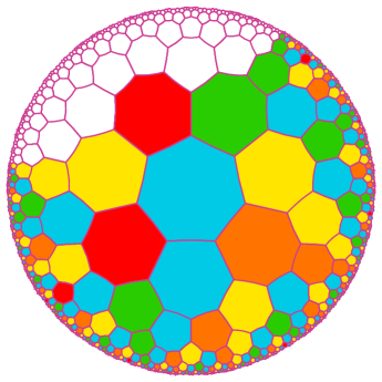
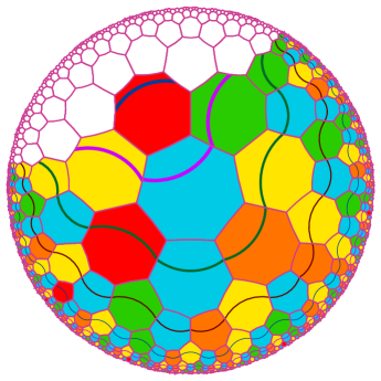
Figure 1: The illustration of the new setting of the construction leading to the proof of the undecidability of the tiling problem in the hyperbolic plane.

The new setting also takes place on the ternary heptagrid, the tiling $\{7,3\}$ of the hyperbolic plane: it is based on the replication of a regular heptagon with $\displaystyle{{2\pi}\over 3}$ as the interior angle by reflection in its sides and then, recursively, by reflection of the images in their sides.

We introduce four colours for the tiles: green, yellow, blue and orange which will be denoted by $G$, $Y$, $B$ and $O$ respectively. We attach the following substitution rules, see [12, 11], as illustrated by the left-hand side picture of Figure 1:

$$G\rightarrow YBG,\ Y\rightarrow YBG,\ B\rightarrow BO,\ O\rightarrow YBO.$$

As noted in [11], this allows to define two types of Fibonacci trees, see [5, 9] for the definition. If we define $B$ to be a black node and $G$, $Y$ and $O$ to be white nodes, we obtain a central Fibonacci tree, see [5, 9]. If we define $G$ and $Y$ to be black and $B$ with $O$ to be white, then we have standard Fibonacci trees. We define seeds as $G$-nodes on an even isocline whose fatheris a $Y$-node and whose grandfather is a $G$-node. In Figure 1, the tree rooted at a seed, in red in the figure, implements the representation of the trees of the mantilla, see [10, 13, 12]. We use this latter interpretation which allows us to construct the isoclines which are the horizontals of our constructions, both for the undecidability of the tiling problem and for the proof of Theorem 1. This is illustrated by the right-hand side picture of Figure 1. The convex arcs are attached to the black nodes, $G$ and $Y$, and the concave ones are attached to the white nodes, here $B$ and $O$.

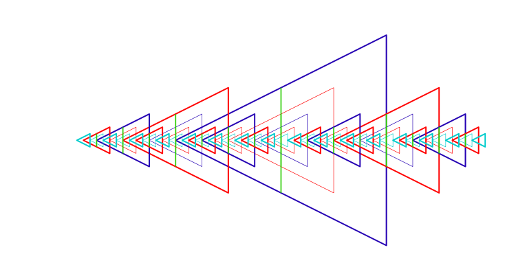
Figure 2: Construction of the interwoven triangles in the Euclidean plane: look at the green signal.

In this new setting, the isoclines are periodically numbered from 0 to 3. We conclude this section by reminding the principle of the interwoven triangles, which is illustrated by Figure 2. The generation 0 is in light blue in the figure. The even generations are in dark blue. Triangles, thick strokes, alternate with phantoms, thin strokes, for each generation. Triangles and only them generate the vertices and the bases of the triangles and phantoms of the next generation: light and dark blue triangles generate the red generations. The red triangles generate the dark blue generations. The reader is referred to [10, 13, 8, 6] for more details on this construction and its implementations in the hyperbolic plane.

3 The mauve triangles

The mauve triangles are constructed upon the interwoven triangles.

The construction of the interwoven triangles needs a lot of signals, which entails a huge number of tiles, still around 9,000 of them in this new context, not taking into account the specific tiles devoted to the simulation of a Turing machine. The construction of this paper requires much more tiles, but we shall not try to count them.

The mauve triangles are constructed from the red triangles of the interwoven ones. Any mauve triangle is triggered by a red triangle and conversely. The vertex of a mauve triangle $T$ is that of a red triangle $R$. Its legs follow those of $R$. After the corner of $R$, they go on, on the same ray, until they meet the basis of the red phantoms which are generated by the basis of $R$. At this meeting, the legs meet the basis of the mauve triangle which coincide with the basis of the just mentioned red phantoms. In [8], we thoroughly describe that this construction can be forced by a finitely generated tiling. We refer the reader to these papers.

3.1 Intersection properties of the mauve triangles

As it stems from a red triangle, we say that a mauve triangle of the generation $n$ is constructed on a red triangle of the generation $2n$+1. Later, it will be useful to recognize the mauve triangles of generation 0: they have the colour mauve-0 and will be called mauve-0 triangles.

From the doubling of the height with respect to the red triangles, the mauve triangles lose the nice property that the red triangles are either embedded or disjoint. This is no more the case for the mauve triangles. However, the overlappings and intersections of mauve triangles can precisely be described.

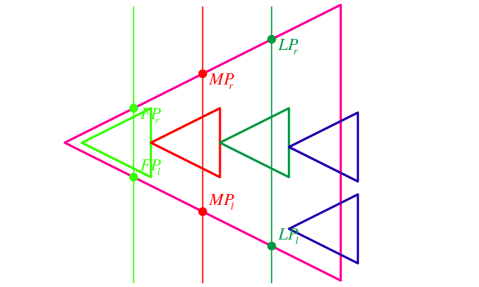
Figure 3: An illustration of the mauve triangles. Inside the big triangle, from left to right, the $0$-, $1$-, $2$- and $3$-triangles of the previous generation.

The figure indicates the first points, $FP$, the mid-points, $MP$, and the low points, $LP$, of a mauve triangle $T$ of generation $n$+1. On Figure 3, we can see that the 3-triangles cut the basis of $T$ at their $LP$’s and that the $LP$’s of the 2-triangles are aligned with those of $T$. The isoclines which pass through the $FP$’s, $MP$’s and $LP$’s of $T$ cut smaller triangles at their $LP$’s and for triangles of generation $n$$-$1 if any, they are cut by these lines if and only if they are 2-triangles. The 3-triangles of the generation $n$ which contains the vertex of $T$, if any, is called the hat of $T$. Note that inside $T$, its 0-triangles are all hatted.

We can see that the intersection between mauve triangles are those which are indicated by Figure 3 and only those. A mauve triangle $T$ intersects 3-triangles of the previous generation: always one of them at its basis, possibly another one near its vertex, at its legs. Also, $T$ may be cut by the basis of a mauve triangle of a bigger generation, always at its $LP$’s. We refer the reader to [14] for a proof of these properties.

3.2 New notions: the $\beta$-clines and the $\beta$-, $\gamma$-points

From the fact that the 3-triangles $T_{i}$’s of the previous generation which are inside a mauve triangle $T$ cut $T$ along its basis and at their $LP$’s, we can see that we can repeat this observation with the 3-triangles of the $T_{i}$’s until we reach mauve-0 triangles. We call $\beta$-cline the isocline of the mauve-0 triangles reached by this process and we say that the $\beta$-cline is attached to $T$. Note that the same isocline is the $\beta$-cline of all the 3-triangles which occur in the just considered construction. By definition, we call $\beta$-points of $T$ the intersection of the legs of $T$ with the $\beta$-cline of the 2-triangles of the previous generation which it contains. Similarly, we call $\gamma$-points of $T$ the intersection of the legs of $T$ with the $\beta$-cline of their hat, if any. Note that if the hat of $T$ does not exist, there are infinitely copies of $T$ within the same set of isoclines which cross $T$ which are hatted, so that for these mauve triangles the $\beta$-cline exist and the considered isocline, the same for all these copies of $T$ also intersect $T$, which allows to define the $\gamma$-points of $T$.

In fact, the $\gamma$-points of $T$ can be constructed in another way, thanks to the following remark. Assume that the hat $H$ of $T$ exists and assume that $T$ belongs to the generation $n$+1. Consider a 0-triangle $Z$ of the generation $n$ which is inside $T$. It is plain that the hat of $Z$ exists if $n>0$, as it is inside $T$ and that it is a 3-triangle of the generation $n$$-$1 which cuts the basis of $H$. Accordingly, $H$ and the hat of $Z$ have the same $\beta$-cline. Consequently, to find the $\gamma$-point of $T$, it is enough to take the intersection of the legs of $T$ with the $\beta$-cline of the hat of $Z$. Note that if $Z$ is a mauve-0 triangle, the considered $\beta$-cline is the isocline which passes through the vertex of $Z$. Consequently, this defines the $\gamma$-points of $T$, independently from the existence or not of the hat of $T$.

Note that the $\beta$-, and $\gamma$-points are not defined for mauve-0 triangles. All the points which we defined in Subsection 3.1 and in this one can be constructed by a small set of signals in terms of tiles.

The constructions relies on the fact that the isoclines joining the $FP$’s and the $MP$’s as well as the basis of $T$ have the following property, assuming that $T$ belongs to the generation $n$+1: if the isocline meets a triangle of the generation $i$ with $i<n$, it is a 2-triangle. This allows to locate the 0-, 1- and 3-triangles of the generation $n$ whose vertex is inside $T$. From this detection, we also can detect the 2-triangles of the generation $n$ which are inside $T$.

Now, we have to indicate how to construct the $LP$’s of $T$ as well as its $\beta$-cline.

The construction of the $LP$’s of $T$ start from the $MP$’s which send two signals: one along the leg of $T$ and another along the isocline joining the $MP$’s, in the direction of the other $MP$. When the horizontal signal meets the vertex of a red phantom, it goes down along it, until it reaches the mid-point $M$ of the leg of the phantom. There, it goes back to the leg of $T$ by following the isocline of $M$, circumventing all triangles which are met from their right-, left-hand side leg, the signal emanating from the left-, right-hand side leg of $T$. In this way, the first leg met by the signal whose laterality is that of the leg from which it came is the expected leg and it also meets the second signal sent by the $MP$.

The construction of the $\beta$-cline of $T$ follows from this construction. A signal leaves each $LP$ of $T$. They go to the opposite side. They follow the leg of $T$, then its basis and then, each time they meet a leg of a 3-triangle at its $LP$, they go down along this leg and, finding the corner, they go along the isocline of the basis of the corner, in the direction of the other corner. This signal is permitted only to go down or to follow an isocline. Consequently, the two considered signals will meet on the isocline which is the $\beta$-cline of $T$, which provides the construction.

The detection of a $\beta$-cline can now be used to construct the $\beta$- and $\gamma$-points, combining the detection of a $\beta$-cline with that of a 0-, or a 2-triangle. The pictures of Figure 4 illustrates the constructions of the $\beta$- and the $\gamma$-points of $T$.

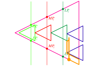
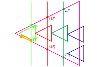
Figure 4: Illustration of the construction of the $\beta$- and $\gamma$-points of a mauve triangle of a positive generation. On the left-hand side: construction of the $\beta$-point. On the right-hand side, construction of the $\gamma$-point.

In [14], we completely prove the following statement:

Lemma 1

The mauve triangles together with the determination of their $LP$’s and mid-points can be constructed from a finite set of prototiles.

which can be established using the above ideas.

The $\gamma$-point allows us to define a last couple of points on the legs of a mauve triangles, the $HP$’s, i.e. high points.

The $HP$’s are defined with respect to the $\gamma$-points as follows. If the $\beta$-cline which crosses the $\gamma$-point is a $\beta$-cline of type 2, then the $HP$ is the $\gamma$-point. If this is not the case, then the $HP$ of $T$ is defined by the first intersection with a basis of a mauve triangle with the legs of $T$, when starting from the $FP$’s and going up towards the vertex. If no basis is met before reaching the vertex, the $HP$ of $T$ is the intersection of the legs with the isocline which is just below that of the vertex of $T$. This is the case for the mauve-0 triangles.

4 A half-plane filling path

Now, we turn to the construction of the path.

As we shall see, the path has no cycle and most often, it consists of a single component which is plane-filling path. In one exceptional situation, the path breaks down into infinitely many infinite components. There is no cycle and each component fills up at least a half-plane.

The points which we defined in the previous section can be seen as signboards which are placed on the path in order to indicate it in which regions it passes and which direction it has to follow.

Our first task consists in describing these regions. In a second step, we shall see how the path fills up the regions, on the basis of an inductive construction.

We define two types of basic regions. The first one is the set of tiles defined by a mauve triangle: its borders and its inside. Remember that the basis of a mauve triangle contains more than the majority of tiles resulting from the just given definition. It is considered as a basic region as once the path enters a mauve triangle $T$, it fills up $T$ almost completely before leaving $T$. In fact, there is a restriction and the path fills a bigger area. Remember that the basis of $T$ is crossed by the legs of a lot of triangles, the 3-triangles of the previous generation whose vertices are inside $T$ and a lot of 2-triangles of smaller generations. The path enters each such triangle $M$ through one of its $LP$’s and it fills it up completely, leaving it through the $HP$ of $M$ which lies on the other leg of $M$. After a while, as will be seen, the path goes back to the basis of $T$ and will meet the next small triangle which crosses this basis. Of course, inside a small triangle filled up by the path, the process is recursively repeated: if the basis of $M$ is crossed by legs of smaller triangles, the path fills them up before going on on the basis of $M$.

This process allows us to define the latitude of a mauve triangle $T$. For a mauve-0 triangle, the lower border is the isocline of the basis of $T$ and it belongs to the latitude. The upper border is the isocline of the vertex of $T$ and it belongs to another latitude. For higher generations, the border of the latitude belonging to the latitude is defined by the isocline of the basis of $T$ with this exception that each time this isocline is crossed by legs of smaller triangles, the border goes down along the legs and then follows the basis of the smaller triangles, repeating this way recursively, until a mauve-0 triangle is reached.

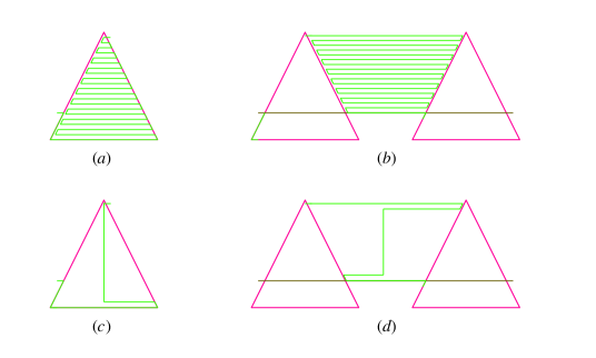
Figure 5: A schematic representation of the path:
On the left-hand side, inside a mauve-0 triangle. On the right-hand side, in between two consecutive mauve-0 triangles within the same latitude when the vertices belong to the same basis.

In Figure 5, the picture $(a)$ illustrates the path inside a mauve-0 triangle and the picture $(b)$ illustrates the path in between two consecutive mauve-0 triangles inside the same latitude. Now, for this situation in between two consecutive mauve triangles of the same latitude, the path fills up the space between the upper and the lower borders. The situation is in general different from the picture $(b)$. Figure 6 describes the general situation for consecutive mauve triangles of generation 1 standing within the same latitude. There, we can see the various configurations which may occur in between consecutive mauve-0 triangles of the same latitude.

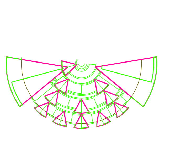
Figure 6: The path in between two triangles of generation $1$.

In Figure 6 we make use of the schematic representation used the pictures $(c)$ and $(d)$ of Figure 5 to represent the pictures $(a)$ and $(b)$. This is repeated in Figure 7 which represents the path inside a mauve triangle of generation 1.

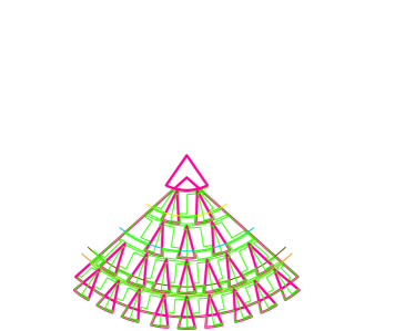
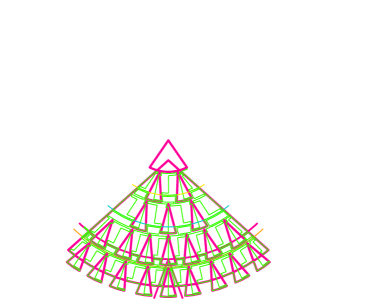
Figure 7: The path inside a triangle of generation $1$.
On the left-hand side: a $0$- or a $1$-triangle. On the right-hand side, a $3$-triangle or a $2$-triangle which is cut by a mauve triangle of a bigger generation.

Other details attached to the path are dealt with in [14] and we refer the reader to this paper.

Now, we notice that Figures 6 and 7 can also illustrate the passage from the generation $n$ to the generation $n$+1. We draw the attention of the reader on the following point. Due to the position of the entry and the exit points for the path in a triangle, the path fills up the bottom part of the triangle which is below the isocline joining its $LP$’s in an almost cycle and then it crosses the other three strips roughly corresponding to 2-, 1- and 0-triangles of the previous generation, in changing its direction each time it enters a new strip. We have a similar feature in between two consecutive triangles of the same latitude. This dictates a difference of behaviour when going to a strip to another. Now, this is regulated by the $\beta$-clines of type 2: they delimit the bottom part of inside a triangle and they delimit the upper one in between two consecutive triangles of the same latitude. As by definition, the intersection of a $\beta$-cline of type 2 with the legs of a triangle define the $HP$ of this triangle, this allows to give a passage to the path for going back to the origin of the almost cycle. The intersection of a $\beta$-cline which is not of type 2 with the legs of a triangle prevent the path to enter the triangle or to exit from it.

With these indications, we conclude that the construction is correct and that the path possesses the following property:

Lemma 2

The path contains no cycle.

Lemma 3

For any tile $\tau$, the path on one side of $\tau$ fills up infinitely many mauve triangles of increasing sizes.

From these lemmas, as established in [14], we get:

Corollary 1

If there are only finite basic regions, the path goes through any tile of the plane.

Now, there is an exceptional situation in which we have infinitely many infinite triangles. In fact, as the path fills up all triangles, the infinite ones included, it splits into infinitely many components which still have no cycle and which fill up the region contained in an infinite triangle and the one in between this infinite triangle and the next one in the same infinite latitude. Now, for these components, Lemmas 2 and 3 are still true, see [14].

5 Proof of the main theorem

We can now prove Theorem 1.

The proof follows the argument of [3], with an adaptation to the case of infinite triangles.

We define a direction for the path constructed in Section 4. To this aim, we introduce three hues in the colour used for the signal of the path. One colour calls the next one and the last one calls the first one. The periodic repetition of this pattern together with the order of the colours define the direction. This allows to define the successor of a tile on the path, which we formalize by a function $\delta$ from $Z\!\!\!Z$ to the tiling such that $\delta(n$+$1)$ is the successor of $\delta(n)$ on the path.

Consider $M$ a deterministic Turing machine with a single head and a single bi-infinite tape which is assumed to be initially empty. From [10, 13], we can define a finite set of tiles $T_{M}$ such that $T_{M}$ tiles the hyperbolic plane if and only if $M$ does not halt. When $T_{M}$ tiles the hyperbolic plane, it defines infinitely many triangles of infinitely many sizes and in each triangle, the simulation of $M$ is resumed from its beginning, running until the basis of the triangle is reached. An automaton $A_{M}$ is attached to $M$ and its states are defined by $D\times\{0,1\}\times T_{M}$, where $D$ is the set of tiles which defines the tiling which we have constructed in Sections 3 and 4. The ${0,1}$-component of a state is called its bit. We can still tile the plane as the tiles of $T_{M}$ are ternary heptagons but the abutting conditions may be not observed: if it is observed with all the neighbours of the cell $x$, the corresponding configuration is said to be correct at $x$, otherwise it is said incorrect. When the considered configuration is correct at every tile for $D$ or at every tile for $T_{M}$, it is called a realization of the corresponding tiling.

As in [3], the transition function does not change neither the $D$- nor the $T_{M}$-component of the state of a cell $x$: it only changes its bit. As in [3], we define $A_{M}(c(x))=c(x)$ if the configuration in $D$ or in $T$ is incorrect at the considered tile. If both are correct, we define $A_{M}(c(x))=\hbox{\rm xor}(c(x),c(\delta(x)))$. It is plain that if $M$ does not halt, $T_{M}$ tiles the hyperbolic plane and there is a configuration of $D$ and one of $T_{M}$ which are realizations of the respective tilings. Then, the transition function computes the xor of the bit of a cell and its successor on the path. Hence, defining all cells with 0 and then all cells with 1 define two configurations which $A_{M}$ transform to the same image: the configuration where all cells have the bit 0. Accordingly, $A_{M}$ is not injective.

Conversely, if $A_{M}$ is not injective, we have two different configurations $c_{0}$ and $c_{1}$ for which the image is the same. Hence, there is a cell $x$ at which the configurations differ. Hence, the xor was applied, which means that $D$ and $T$ are both correct at this cell in these configurations and it is not difficult to see that the value for each configuration at the successor of $x$ on the path must also be different. And so, following the path in one direction, we have a correct tiling for both $D$ and $T_{M}$. Now, from Lemma 3, as the path fills up infinitely many triangles of increasing sizes, this means that the tiling realized for $T_{M}$ is correct in these triangles. But, in each triangle, the computation of $M$ is simulated from its beginning. Accordingly, the Turing machine $M$ never halts. And so, we proved that $A_{M}$ is not injective if and only if $M$ does not halt. Accordingly, the injectivity of $A_{M}$ is undecidable.  

6 Conclusion

In the Euclidean plane, the surjectivity of the global function of cellular automata is tightly connected with the injectivity of the function. This is not the case in the hyperbolic plane, see [15], so that the question of the surjectivity is open in this case. Note that the present construction can be generalized to any grid $\{p,3\}$ of the hyperbolic plane, with $p\geq 7$.

References

- [1] Berger R., The undecidability of the domino problem, Memoirs of the American Mathematical Society, 66, (1966), 1-72.
- [2] Goodman-Strauss, Ch., A strongly aperiodic set of tiles in the hyperbolic plane, Inventiones Mathematicae, 159(1), (2005), 119-132.
- [3] Kari J., Reversibility and Surjectivity Problems for Cellular Automata, Journal of Computer and System Sciences, 48, (1994), 149-182.
- [4] Kari J., The Tiling Problem Revisited, Lecture Notes in Computer Science, 4664, (2007). 72-79.
- [5] M. Margenstern, New Tools for Cellular Automata of the Hyperbolic Plane, Journal of Universal Computer Science 6(12), (2000), 1226–1252.
- [6] Margenstern M., The Domino Problem of the Hyperbolic Plane Is Undecidable, arXiv, (2007), June, 18p.
- [7] M. Margenstern, On a characterization of cellular automata in tilings of the hyperbolic plane, ACMC’2007, Aug. 2007, Budapest, (2007)
- [8] Margenstern M., Constructing a uniform plane-filling path in the ternary heptagrid of the hyperbolic plane, arXiv, (2007), October, 22p.
- [9] Margenstern M., Cellular Automata in Hyperbolic Spaces, Volume 1, Theory, OCP, Philadelphia, (2007), 422p.
- [10] Margenstern M., The Domino Problem of the Hyperbolic Plane is Undecidable, Bulletin of the EATCS, 93, (2007), October, 220-237.
- [11] Margenstern M., About the periodic tiling problem in the hyperbolic plane and connected questions, Conference on Computational and Combinatoric aspects of Tilings, Imperial College, London (UK), July, 31- August 1, 2008.
- [12] Margenstern M., Cellular Automata in Hyperbolic Spaces, Volume 2, Computations and Implementations, OCP, Philadelphia, to appear 2008, 362p.
- [13] Margenstern M., The domino problem of the hyperbolic plane is undecidable, Theoretical Computer Science, in press, doi: 10.1016/j.tcs.2008.04.038, 56p.
- [14] Margenstern M., The injectivity of the global function of a cellular automaton in the hyperbolic plane is undecidable, arXiv:, (2008), June, 29p.
- [15] Margenstern M., Cellular Automata in hyperbolic spaces: new results, AUTOMATA’2008, June, 12-14, 2008, Bristol, UK, invited talk.
- [16] M. Margenstern, K. Morita, NP problems are tractable in the space of cellular automata in the hyperbolic plane, Theoretical Computer Science, 259, 99–128, (2001)
- [17] Robinson R.M. Undecidability and nonperiodicity for tilings of the plane, Inventiones Mathematicae, 12, (1971), 177-209.