A Sample of Candidate Radio Stars in FIRST and SDSS
Abstract
We conduct a search for radio stars by combining radio and optical data from the Faint Images of the Radio Sky at Twenty cm survey (FIRST) and the Sloan Digital Sky Survey (SDSS). The faint limit of SDSS makes possible a homogeneous search for radio emission from stars of low optical luminosity. We select a sample of 112 candidate radio stars in the magnitude range and with radio flux mJy, from about 7000 deg2 of sky. The selection criteria are positional coincidence within , radio and optical point source morphology, and an SDSS spectrum classified as stellar. The sample contamination is estimated by random matching to be , suggesting that at most a small fraction of the selected candidates are genuine radio stars. Therefore, we rule out a very rare population of extremely radio-loud stars: no more than 1.2 of every million stars in the magnitude range stars has radio flux mJy. We investigate the optical and radio colors of the sample to find candidates that show the largest likelihood of being real radio stars. The significant outliers from the stellar locus, as well as the magnetically active stars, are the best candidates for follow-up radio observations. We conclude that, while the present wide-area radio surveys are not sensitive enough to provide homogeneous samples of the extremely rare radio stars, upcoming surveys which exploit the great sensitivity of current and planned telescopes do have sufficient sensitivity and will allow the properties of this class of object to be investigated in detail.
1 INTRODUCTION
The light from stars dominates the optical sky, while the radio sky’s contribution from stars is very small. However, significant radio emission has been detected from active stars in the form of synchrotron, gyrosynchrotron, or electron cyclotron maser emission (Dulk, 1985; Güdel, 2002). Some of the non-thermal processes that lead to these types of emission— plasma heating and particle acceleration in stellar coronae— are seen in our own Sun, but the relevant energies for active stars are much larger. Radio emission at the relative level of that emitted by the Sun remains undetected from even the closest solar-type main sequence stars to the present day.111Typical radio flux from a star identical to the Sun, and with apparent magnitude , would reach about mJy. The quiescent, slowly varying radio emission seen in many active stars (e.g. Güdel, 2002, and references therein) has no solar counterpart.
With the great increase in the sensitivity of radio surveys in the last several decades, along with the more accurate source positions allowed by radio interferometry, both thermal and non-thermal radio emission have now been detected from hundreds of stars of many different types (Hjellming & Gibson, 1986; Wendker, 1987; Altenhoff et al., 1994; Wendker, 1995; Taylor & Paredes, 1996). These include pre-main-sequence stars (T Tau and Herbig Ae/Be222The “e” following the spectral class indicates emission in the spectrum. stars; Güdel et al., 1989; White et al., 1992; Skinner et al., 1993), rapidly-rotating main-sequence stars (Lim & White, 1995; Berger, 2002), X-ray bright main sequence stars (Güdel et al., 1995), magnetic stars (Drake et al., 1987a; Leone et al., 1996; Berger, 2006; Berger et al., 2008), cool giants with extended chromospheres and photospheres (Newell & Hjellming, 1982; Drake & Linsky, 1986; Drake et al., 1987b; Knapp et al., 1995; Reid & Menten, 1997), OB stars with winds (Bieging et al., 1989; Drake, 1990; Phillips & Titus, 1990), Wolf-Rayet stars (Chapman et al., 1999), dMe flare stars (White et al., 1989; Osten et al., 2006), and various classes of interacting binaries and cataclysmic variables. The radio radiation from these stars is very faint, at the few mJy level.
The first large unbiased study of radio stars ( of sky at high galactic latitude) was performed by Helfand et al. (1999, hereafter H99), who compared the Faint Images of the Radio Sky at Twenty cm survey (FIRST; Becker et al., 1995) to several catalogs of bright stars with high astrometric precision: the Hipparcos catalog (Perryman et al., 1997), the Tycho catalog (Hoeg et al., 1997), the Guide Star Catalog (Lasker et al., 1990), and stars within 25 pc of the Sun. They emphasize the need for accurate positions: the rarity of radio stars to the FIRST flux limit ( 1 mJy), combined with the high density of faint extragalactic radio sources, ensures random matches between stellar and radio sources in sufficient numbers to confuse the cataloging of true radio stars, unless both radio and optical positions are known to better than . H99 identified 26 radio stars in their study, about one per , and showed that the fraction of stars with radio emission above the FIRST limit declines steeply with optical magnitude to . The fraction of radio stars at fainter magnitudes is unknown. Kimball & Ivezić (2008, hereafter KI08) searched for radio stars in a combined radio—optical catalog with observations from FIRST and from the optical Sloan Digital Sky Survey (SDSS). Quasars are the most common radio source above flux densities of a few mJy; therefore a sample of optical point sources with radio emission is likely to be srongly dominated by quasars. KI08 approached this problem by applying a conservative photometric color cut, using the fact that quasars and stars lie in different locations in SDSS optical color-color diagrams (Richards et al., 2001). The sample was limited to sources sufficiently bright to be included in the SDSS quasar spectroscopic target selection (, Schneider et al., 2007). Only 20% of the photometrically-selected candidate radio stars actually showed stellar spectra, while the rest were quasars with stellar-like colors. KI08 concluded that simple color critera are not sufficient to select a clean sample of radio stars, and that spectroscopic observations are necessary to distinguish between quasars and stars.
In this paper we continue the search for radio stars in the SDSS using a sample with spectroscopic identifications. We present 112 candidates selected by matching FIRST detections and SDSS point sources within 1 arcsec. The sample comprises sources brighter than in the optical and 1.25 mJy at 20 cm, with SDSS spectra classified as stellar both by the automated reduction pipelines and visually. The SDSS spectroscopic targeting implicitly imposes soft magnitude limits of . In this magnitude range, approximately 1% of SDSS stars have spectroscopic data. However, all objects in this range which are close to a FIRST source are targeted for spectra (Stoughton et al., 2002), so the completeness of SDSS radio—optical sources is well understood.
We are searching in a different region of the radio—optical parameter space from H99, who also matched to FIRST but used optical catalogs brighter than . The SDSS has a saturation limit of . By extending to several optical magnitudes fainter than H99, we are therefore searching for stars with a much brighter radio-to-optical flux ratio. However, a FIRST—SDSS matching has the potential to reveal a radio-bright population too rare to appear in the smaller H99 study, as the fainter SDSS includes a much larger volume in the Galaxy. For example: M dwarfs, many of which are known to be magnetically active (e.g., West et al., 2008), are found in significant numbers only at faint magnitudes. Thus, a search for radio-emitting M dwarfs should be carried out in a deep optical survey with large sky coverage. Advantages to using the SDSS are its high completeness, precise magnitudes, accurate astrometry, much deeper optical data than previous stellar catalogs, and almost 300,000 stellar spectra.
The remainder of the paper is laid out as follows. In §2 we describe the contributing surveys. In §3 we outline the selection of the sample of radio stars and place an upper limit on the fraction of radio stars. In §4 and §5 we discuss optical and radio properties of the sample, respectively, and in §6 we conclude and summarize our results.
2 OPTICAL AND RADIO DATA
2.1 Optical Catalog: SDSS
We have drawn our sample from the photometric coverage of the sixth data release (DR6) of the Sloan Digital Sky Survey333The survey website is located at http://www.sdss.org. (SDSS; see York et al., 2000; Stoughton et al., 2002; Adelman-McCarthy et al., 2008, and references therein). DR6 covers roughly and contains photometric observations for 287 million unique objects, as well as spectra for more than 1 million sources (in a smaller sky area of ). SDSS entered routine operations in 2000; DR6 observations were completed in June 2006. Because SDSS spectroscopy is performed after photometric observations, some stars in the sample have spectra that were not available until the Seventh Data Release (DR7). We have included some stars with DR7 spectra444We include stars with spectroscopic observations taken through 5 Dec 2007.; we point out explicitly where this detail affects our estimates of sample contamination in §3.6. The DR6 sample includes about 287,000 spectra classified as stars.
The SDSS photometric survey measures flux densities nearly simultaneously in five wavelength bands (, , , , and ) with effective wavelengths of 3551, 4686, 6165, 7481, and 8931Å (Fukugita et al., 1996; Gunn et al., 1998; Hogg et al., 2001; Tucker et al., 2006; Smith et al., 2002; Ivezić et al., 2004). Morphology information allows reliable star—galaxy separation to (Lupton et al., 2002; Scranton et al., 2002). Sources are classified as resolved or unresolved using a measure of light concentration that determines how well the flux resembles a point source (Stoughton et al., 2002). Magnitudes were corrected for Galactic extinction according to the dust maps of Schlegel et al. (1998). The astrometry of the photometric survey is good to (Pier et al., 2003).
A subset of photometric sources was chosen for spectroscopy according to the SDSS targeting pipeline; stars could be serendipitously selected by any of the various targeting algorithms. The quasar targeting algorithm selects all sources within of a FIRST catalog object, and some sources as faint as (depending on the availability of spectral fibers). About 30% of quasar targets turn out to be stars or galaxies (Schneider et al., 2007). Another algorithm targets interesting stellar classes by selecting for their distinctive photometric colors; these include blue horizontal-branch stars, carbon stars, subdwarfs, cataclysmic variables, brown and red dwarfs, and white dwarfs. Because stars in these catagories are selected randomly to fill excess spectral fibers, the completeness of the samples of stars with spectroscopic observations is, with a small number of exceptions, not well-defined. However, the fact that all objects within of a FIRST source are targeted implies that the spectroscopic sample is complete to with respect to radio—optical sources brighter than the FIRST limit, except in the case of fiber collisions (see below).
SDSS spectra are obtained using fibers in a fiber-fed spectrograph (Newman et al., 2004). Spectra cover the wavelength range from about 3500 to 9500 Å with a resolution of R1800. They are automatically extracted and calibrated by the Spectroscopic Pipeline: wavelength calibrations are calculated from arc and night sky lines and flux calibrations from observations of standard F stars. Some fibers are used to observe blank sky in order to correct targeted objects for the sky spectrum. Not every object targeted for spectroscopy obtains a spectrum, primarily because of fiber collisions: due to the physical size of the fibers, no two fibers can be placed closer than on a spectroscopic plate. As a result, spectra are only taken for about 92.5% of spectroscopic targets, although the completeness effects are well understood (Blanton et al., 2003).
2.2 Radio Catalogs
FIRST provides 20 cm radio fluxes, which were used to select candidate radio stars. The Westerbork Northern Sky Survey and the Green Bank 6 cm survey provide fluxes at 92 cm and 6 cm, respectively, which allow us to determine a radio spectral shape.
2.2.1 FIRST
The Faint Images of the Radio Sky at Twenty cm survey (FIRST; Becker et al., 1995) used the Very Large Array to observe the sky at 20 cm (1.4 GHz) with a beam size of 54 and an rms sensitivity of about 0.15 mJy beam-1. Designed to cover the same region of sky as the SDSS, FIRST observed at the North Galactic Cap and a smaller wide strip along the Celestial Equator from 1994 to 2002. The survey contains over 800,000 unique sources, with positions determined to ; its source density is roughly . It is 95% complete to 2 mJy and 80% complete to the survey limit of 1 mJy. The integrated flux density, , is calculated using a two-dimensional Gaussian fit to each source image.
2.2.2 WENSS
The Westerbork Northern Sky Survey (WENSS; Rengelink et al., 1997) is a 92 cm radio survey that was conducted in the mid-1990s. It observed the sky north of to a limiting flux density of 18 mJy, with a beam size of and a positional uncertainty of –.
2.2.3 GB6
The GB6 survey at 4.85 GHz (Green Bank 6 cm survey; Gregory et al., 1996) was executed with the original 91m Green Bank telescope in 1986 November and 1987 October. Data from both epochs were assembled into a survey covering the sky down to a limiting flux of 18 mJy, with resolution and a positional uncertainty of –.
3 SELECTING A SAMPLE OF CANDIDATE RADIO STARS FROM FIRST AND SDSS

This section outlines the selection criteria that yield the candidate radio stars sample. We estimate the amount of contamination with random matching, and use the result to place an upper limit on the fraction of radio stars in the magnitude range of the sample. The area of overlap of the two surveys is about 9500 deg2.
3.1 Magnitude and flux limits
We applied magnitude/flux limits as a way to control source quality. For SDSS sources, we required to ensure reliable determination of optical morphology, as well as to select sources with a high enough signal-to-noise ratio (S/N) for spectral typing. Owing to the magnitude limits of the SDSS quasar target selection algorithm (§2.1), most of the sources in the final sample have , although it is not an explicit requirement. There are roughly 4000–5000 SDSS sources with per square degree on the sky, depending on Galactic latitude.
For the radio sources, we adopted a limit of mJy (equivalent to AB magnitude 16.2). This is slightly brighter than the 1 mJy depth of the FIRST catalog; however, in a visual examination of faint FIRST images, many sources fainter than this appeared to be possibly spurious detections. Above this flux limit, there are about 82 FIRST sources per square degree.
3.2 Positional matching of point sources
We restricted the sample to optical point sources using SDSS automated star—galaxy separation (§2.1). Figure 1 shows the distribution of FIRST—SDSS distance for radio—optical (point source) matches. The expected contamination by random matches (evaluated by off-setting the FIRST positions by in right ascension) is also shown. The inset plot shows the estimated completeness (solid line; percentage of physical sources recovered) and efficiency (dotted line; percentage of all matches which are physical) as a function of matching radius. The precise choice of matching radius is a tradeoff between sample completeness and sample contamination. Since we are looking for rare objects, we opted more on the side of decreased contamination, and chose to use a matching radius. As shown in Figure 1, the matching radius of results in 96% completeness and 98% efficiency. There are 2000–3000 SDSS point sources per square degree with . Correlating with FIRST positions within resulted in matches.
We did not consider proper motions when matching the two catalogs, but emphasize that this decision should not significantly affect the matching results. All of the observations were performed since 1994. Within the relevant magnitude range, nearly 99% of SDSS stars have an apparent motion of less than 0.1 arcsec yr-1, with a median value mas yr-1. Proper motions555Proper motions were determined from the Seventh Data Release of SDSS following the procedure of Munn et al. (2004). for this sample are much smaller than for the sample of H99 owing to the much fainter flux limit and correspondingly larger source distances.
3.3 Spectral typing
KI08 showed that a sample of potential radio stars selected by their SDSS colors is strongly contaminated by quasars. There are enough quasars with stellar colors (i.e., within a few hundredths of a magnitude from the main stellar locus in the multi-dimensional SDSS color space) that spectroscopic identifications are necessary in order to cull them from the sample. We therefore required an SDSS spectroscopic observation for each matched source, and limited the sample to those with stellar-classified spectra. Of the selected matches, 6413 have spectra, and 292 of those were classified as stellar by the SDSS spectral processing pipeline.
For a more robust determination of spectral type, we executed visual classification of each spectrum. Of the 292 stellar-classified sources, 6 matched to known quasars (Schneider et al., 2007) and 45 to known BL Lac objects (Plotkin et al., 2008). We removed one object whose spectrum showed broad emission lines signifying the super-position of a star with a quasar. Of course these false matches are not indicative of an 18% failure rate for the spectral pipeline, which is optimized to detect galaxies, stars, and quasars rather than rare sources such as BL Lac objects. Because the selection criteria for this study are biased toward (radio) quasars, they result in a disproportionately large number of BL Lac objects, which make up a very tiny percentage of the entire SDSS spectroscopic database.
Spectral types were individually assigned to the remaining 240 sources using a custom IDL package dubbed “the Hammer”.666http://www.cfa.harvard.edu/kcovey/thehammer The full algorithm used by the Hammer is described in Appendix A of Covey et al. (2007). In short, the Hammer automatically types input spectra by measuring a suite of spectral indices and performing a least-squares minimization of the residuals between the indices of the target and those measured from spectral type standards. It then allows a confirmation or correction of spectral type according to a visual comparison of the input spectrum with spectral templates. Although spectral types are available from the SDSS database, visual confirmation by stellar scientists (authors GRK, AAW, JJB) leads to more robust classifications.
With visual classification, the sample was reduced to 194 sources with reliable stellar spectra. The rejected spectra were too noisy for reliable typing, or were indicative of BL Lac objects. The latter are not included in the BL Lac sample of Plotkin et al. (2008); that sample was drawn from SDSS Data Release Five (DR5), and thus covers a smaller sky area than the DR6 sample used in this paper.
3.4 Visual examination of radio morphology
We looked at FIRST images of the remaining sample in order to determine the radio morphology of each source. We anticipated that the majority would be point sources, because the resolution of FIRST () is not sufficient to resolve stellar emission. Resolved or multiple-component emission, however, would be strongly indicative of a non-stellar source such as an active galactic nucleus (AGN) with radio jets.
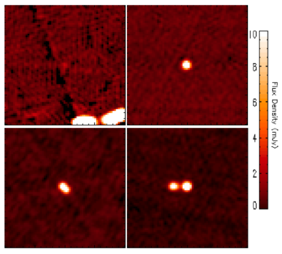
We examined FIRST postage stamps (), and classified each as “compact” (point source emission), “resolved” (resolved single-component emission), “complex” (multiple-component or knotty emission), or “spurious” (e.g., an artifact introduced by interferometric errors). An example from each category is shown in Figure 2. Resolved or complex radio morphology is typically associated with an extra-Galactic object such as a radio galaxy or quasar.777Galactic objects such as HII regions or supernova remnants may show extended emission; however we do not expect contamination from these sources because our sample is limited to or more above the Galactic plane. Out of the 194 visually-classified images we found six spurious sources, which were removed from the sample. Of the remaining 188 sources, 60 are complex, 16 are resolved, and 112 are compact.888For one source that was initially identified as “complex”, the optical image shows a nearby galaxy that appears to be the source of the second point of radio emission. We concluded that the two radio components are physically unrelated, and moved that object into the “compact” category, leading to the totals given in the text. The high fraction of sources with complex radio emission demonstrates that many radio quasars survived the previous selection criteria. Because these objects clearly show stellar spectra, we interpret them as optically-faint radio quasars in chance alignment with bright foreground stars. We rejected the complex sources as obviously extra-Galactic. However, not all quasars have complex radio emission from detectable lobes, but many are instead point sources (KI08): this is typically thought to be the result of Doppler beaming of a jet aligned along the line of sight. Thus, despite the thorough visual classifications, the final set of compact radio sources with stellar spectra may remain contaminated by chance star—quasar superpositions. We discuss sample contamination in more detail in §3.6.
3.5 Final sample of potential radio stars
We retain the sample of 112 compact sources for the remaining analysis of this paper. This set of radio star candidates is presented in Table 1, which lists positions, stellar type, radio fluxes, optical magnitudes, and radio morphology classification. The 16 resolved sources and 60 complex sources are listed in Tables 2 and 3, respectively. The tables also list the distance to each star, calculated using the photometric parallax relation of Ivezić et al. (2008a); this relation is valid only for stars on the main sequence. As discussed by Finlator et al. (2000), nearly all SDSS stars () are expected to lie on the main sequence. However, it is possible that by selecting radio-emitting stars we have biased our sample toward giant stars in the halo (nearby giants are brighter than the SDSS saturation limit). We note that approximately 40% of the candidate radio stars have measured by the SDSS software pipeline; all have , indicating that they are main sequence stars. There is no evidence that the sample has a different distance distribution than other SDSS stars with spectra.
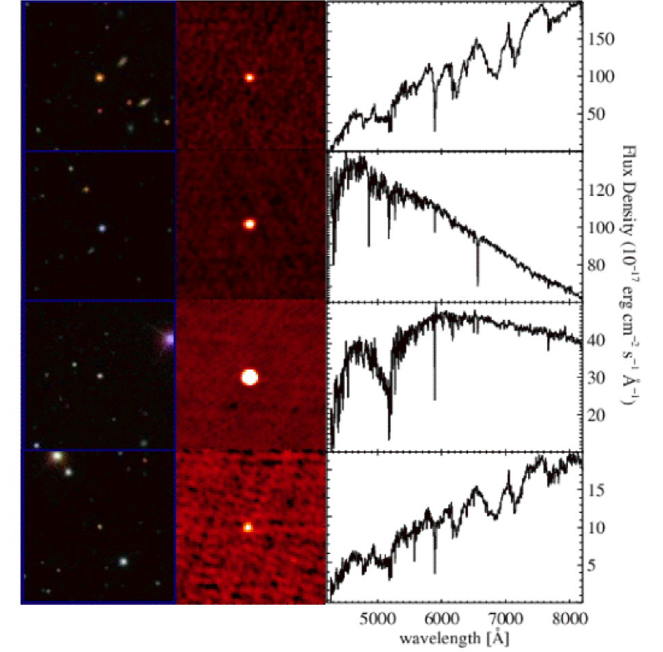
Figure 3 is a mosaic of four of the candidate radio sources; it shows the optical image, the radio image, and the optical spectrum for each one. The brightest optical source and the brightest radio source in the sample are included in the mosaic.
3.6 Estimating Sample Contamination
To estimate the contamination originating from chance radio—optical alignments, we created a set of twelve random samples for comparison. To create the random samples, we off-set the right ascension or declination in the FIRST catalog (by , , , , , or degree), then applied identical selection criteria (where possible) as above. The contamination estimate is an upper limit because it is not possible to apply exactly the same selection criteria to the random samples: the SDSS spectral target selection for quasars (§2.1) ensures that a large fraction of the real FIRST—SDSS matches have spectral data, whereas very few sources in the random samples have SDSS spectra.
Having performed the matching several times, we can determine the variance of the random sampling. 999Varying the FIRST positions results in a slight decrease of the areal overlap between FIRST and SDSS. However, given that so few matches result from the random sampling, the small change in matching area has no significant effect on the contamination estimate. Random matching of all FIRST and photometric SDSS sources resulted in matches. Applying the magnitude and radio flux limits reduced the samples to matches. Selecting on optical point source morphology further reduced the samples to .
The next selection step for the real sample was to eliminate those sources without SDSS spectra. The equivalent step for the random samples is to eliminate those which could not have qualified for SDSS spectral targeting. The quasar targeting algorithm (§2.1) depends on proximity to a radio source; by artificially shifting the FIRST positions to create the random samples, we created fake optical—radio sources which would pass the selection criteria. We rejected sources outside of the DR6 spectroscopic coverage, which is smaller than the DR6 photometric coverage. Keeping only those matches which would qualify for SDSS spectroscopy reduced the random samples to . Applying the success rate of spectral sampling of SDSS targets (92.5%; Blanton et al., 2003) results in an expected random sample size of .
We can make an educated guess that the remaining random samples consist almost entirely of stars: at these very bright magnitudes, the SDSS star—galaxy separation mechanism is quite effective at differentiating between point sources and extended sources. Besides stars, the most common type of optical point source is a quasar, but these are rare at . For example, the highest fraction of quasars in SDSS can be found at the North Galactic Pole, where there are about 100 stars for each quasar (at magnitudes ; Jurić et al., 2008). Close to the Galactic plane, the quasar fraction is much smaller.
The final step in the selection process was to visually classify each source according to its radio morphology. Only those objects which appeared by eye to be unresolved in their FIRST image were retained. Selecting these objects results in a random sample size of . Applying the spectral observation success rate reduces that value to . Estimating one per cent of the sample are quasars as described above, the final estimate is . This number is essentially identical to the size of the candidate radio stars sample, which consists of 104 stars from DR6 and 8 additional stars with spectroscopy performed later than that of DR6.
The above comparison shows that most or all of the potential radio stars are actually chance alignments of SDSS stars with unrelated FIRST sources. The variance in the random samples is large enough that there may be several real radio stars in the candidates sample or none at all. This result indicates that radio stars are extremely rare or non-existant in the range , mJy.
3.7 The Fraction of Radio Stars in the SDSS
We can use the relative sizes of the candidate and random samples, along with the sample completeness, to calculate an upper limit on the fraction of radio stars in the SDSS. The candidate sample contains 104 stars with spectra in DR6; 98 of those are in the magnitude range . As discussed previously, the estimated number of contaminating sources is . We can therefore state with 97.5% confidence that there are no more than 16 radio stars in the sample of candidates (using the one-sided 2- error estimate). The completeness estimate has the following contributions: 1) the completeness of the FIRST survey at 1.25 mJy is approximately 85–90% (Becker et al., 1995); 2) the completeness of the radio—optical matching within is 96%; 3) the SDSS spectroscopic targeting algorithm selects all objects within of a FIRST source (100% completeness); 4) given fiber collisions, the success rate of spectroscopic observations is about 92.5%101010The success rate is not biased with respect to the radio sample; we verified that approximately 92.5% of our selected sources which should have passed the targeting selection do in fact have SDSS spectra. (Blanton et al., 2003). We therefore estimate that the sample is about 75% complete, and thus that there are no more than 21 radio stars in the SDSS DR6 with . There are approximately 18 million SDSS stars in this magnitude range, which implies that no more than 1.2 out of every million stars in the range have a radio flux of 1.25 mJy. For stars with , that corresponds to an upper limit on radio to optical flux ratio of 0.34; for the stars at the faint end, the upper limit on radio to optical flux ratio is 15.
4 OPTICAL PROPERTIES
We showed in the previous section that the sample is highly contaminated by interloping AGN. However, statistical comparisons of the sample with typical stars can highlight the most likely actual radio stars. In this section, we examine optical properties of the sample: photometric colors, distance from the stellar locus, spectral type, and magnetic activity. We also use an SDSS control sample selected from a strip of sky wide in right ascension. The control sample contains point sources with and from the region , ; it contains just over 160,000 sources.
4.1 Photometric colors
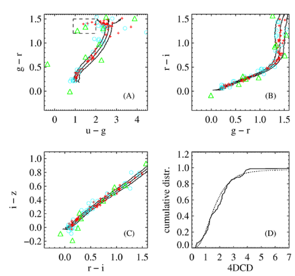
Figure 4 presents the distribution of the candidate radio stars in optical color—color space, compared to the SDSS stellar locus as parameterized by Covey et al. (2007). The majority of the candidate stars lie on the stellar locus. Several stars, however, appear to lie along the white-dwarf—M dwarf (WD+dM) bridge (Smolčić et al., 2004): . Such close binary pairs are found to be more active than their single field counterparts (e.g., Silvestri et al., 2005, 2006). Smolčić et al. (2004) limited their analysis to stars with to eliminate those with poor photometry. In the SDSS control sample, less than 0.1% of stars lie on the WD+dM bridge. The candidate radio stars sample contains seven stars which lie along the WD+dM bridge, corresponding to a much higher fraction. We note however that all of our WD+dM candidates have -band magnitudes ; therefore -band photometry may have artificially moved these sources blueward of the M star locus (upper right corner of the stellar locus). None of their spectra suggest the presence of a white dwarf companion. We note that the star with is not on the WD+dM bridge, as it has . However, the spectrum and photometric image do suggest that it is a (physical or optical) binary system: a K3 star with an added blue component.
A quantitative method of finding outliers from the stellar locus, taking photometric errors into account, is outlined by Covey et al. (2007). They parameterized the stellar locus by finding its 1- width in the standard SDSS colors () and Two-Micron All Sky Survey (Skrutskie et al., 2006) colors as a function of . They chose as the fiducial color because it samples the largest wavelength range possible without relying on the shallower or measurements. Using only the SDSS colors, we define a “four-dimensional color distance” (4DCD; analogous to the seven-dimensional version discussed in C07111111Our definition of differs from C07 by a square root operator, such that our value is in the units of a color distance.), which describes the statistical significance of the distance in color space between a target object and the point on the stellar locus with the same color as the target. The 4DCD is defined by
| (1) |
where , , etc. The width of the stellar locus is , which refers to the FWHM of the locus in color at the same as the target object. The error in the target’s color, , is calculated by adding in quadrature its photometric errors in the two appropriate filters.
We characterize outliers from the stellar locus as those with a value of 4DCD greater than two, shown as circles in Figure 4. Extreme outliers, with 4DCD, are shown as triangles. Three of the stars with WD+dM colors have 4DCD; these are strong candidates for further investigation. The lower right panel compares the cumulative distributions for the candidate radio stars (full line) and the SDSS control sample; the two distributions are similar. The largest 4DCD value of belongs to the possibly binary star mentioned earlier, having . The other most extreme outlier has 4DCD . The spectrum of that object also shows some evidence that the source is part of a multiple system, such as the super-position of a late-type with an early-type M star. All other values of 4DCD are .
4.2 Spectral type and activity fraction
Because non-thermal radio emission is a signal of activity, we expect that radio emission may correlate with strong spectral lines, such as H, which are also known to signal magnetic activity. We investigate the fraction of active stars in our sample; if the sample contains some real radio stars which are active, we may see an increase over the active fraction of all stars (without selecting for radio emission). Previous studies have found that the fraction of active M dwarfs is a strong function of spectral type (West et al., 2004, 2008), tending to increase toward later subtypes with a peak around M8 dwarfs.
An H equivalent width was measured for each stellar spectrum using the Hammer (§3.3). As discussed by West et al. (2008), the accuracy of such measurements has been tested via Monte Carlo simulations to ascertain how well line strength can be determined at a given S/N level. The H emission can be recovered over 96% of the time for all spectral types. Figure 5 shows the spectral types of the candidate radio stars sample (solid line), compared with all SDSS DR6 stars with spectra (just under 1 million stars; dotted line). Spectral types for the SDSS sample come from the automated version of the Hammer, while spectral types for the candidate radio star sample were visually-confirmed (§3.3). Automated Hammer classifications are typically accurate to within subtypes for A–G stars, and within subtypes for K and M stars (Covey et al., 2007). All spectra for the radio stars sample have S/N ratio greater than 2.9. As shown in Figure 5, all of the active candidate radio stars are M dwarfs. This is not a surprising result given that most stars are M dwarfs (Covey et al., 2008; Bochanski et al., 2009), and the majority of activity in main sequence stars is seen in M dwarfs (e.g., Gizis et al., 2002). West et al. (2008) discussed the fraction of active M dwarfs in SDSS DR5 as a function of spectral subtype, after removing WD+dM bridge stars from their sample. They found that M0–M3 stars have an active fraction of roughly 5–20%, and that the fraction increases strongly for M dwarfs of later subtype. Our results for the candidate radio stars are consistent with the results of that study for all stars; we do not see a significantly higher fraction of active stars in the sample of candidate stellar radio sources.
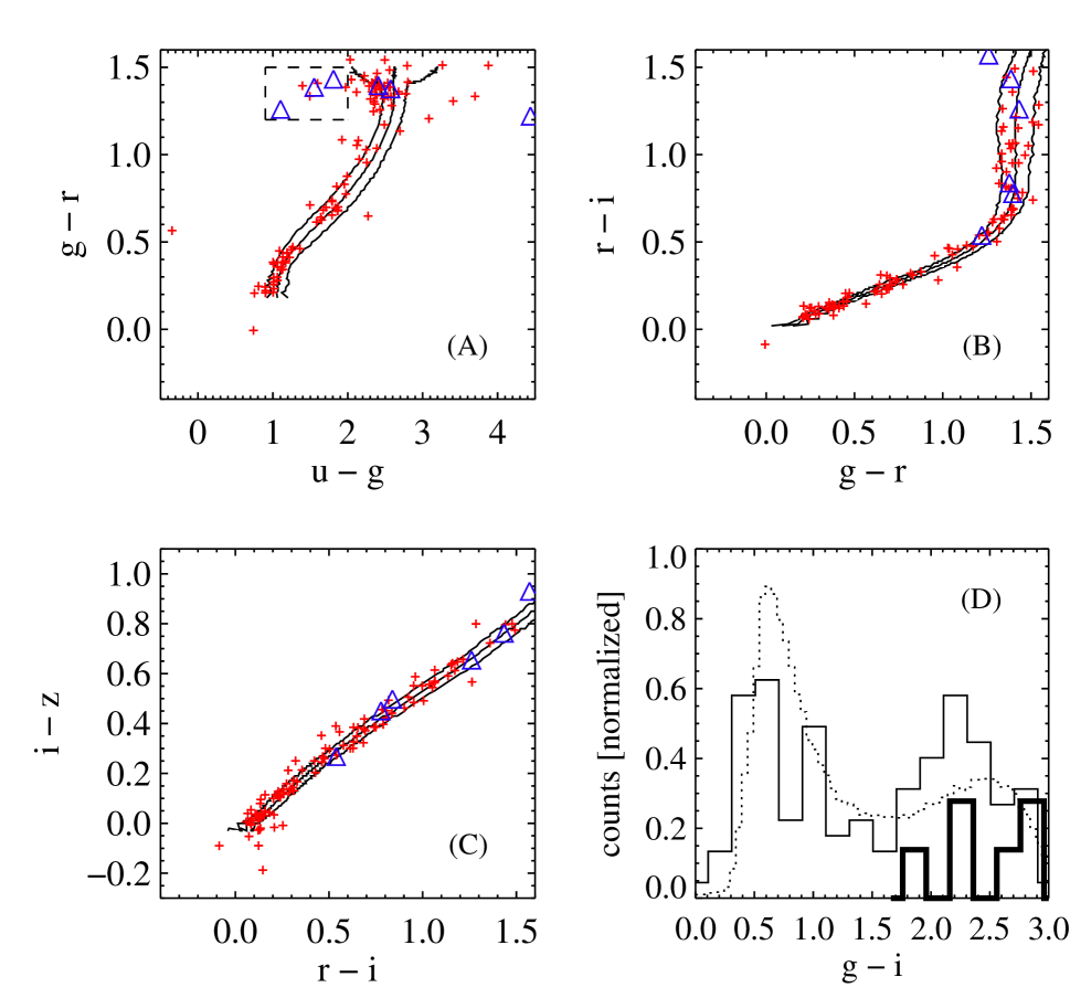
Figure 6 shows color—color diagrams of the candidate radio stars and the SDSS control sample, with the six active stars indicated by triangles. Three of the seven stars with WD+dM bridge colors (§4.1) are active; two of those are outliers from the stellar locus (4DCD ). This result is in agreement with Silvestri et al. (2006), who suggest that 20-60% of all WD+dM binaries are magnetically active. The lower right panel of Fig. 6 shows the distribution of the SDSS control sample (dotted line), the candidate radio stars (thin solid line), and the active stars (thick solid line). Covey et al. (2007) showed that correlates strongly with stellar spectral type. The distribution is bimodal in flux limited samples: it is biased toward red stars, which are the most common, but also blue stars, which can be seen from much greater distances. West et al. (2004) and Bochanski et al. (2007) compared the colors of active to inactive M dwarfs in the field (i.e., not part of a binary system). They found no significant differences between the two populations. The current radio stars study includes three active field M dwarfs (i.e., M dwarfs which do not have WD+dM bridge colors). Although the sample is too small to make a strong statement in comparison with the studies of West et al. (2004) and Bochanski et al. (2007), we note that our results for stars with radio emission are consistent with their conclusions for all stars.

5 RADIO PROPERTIES
5.1 Radio Spectral Slope
Using the multiple-wavelength radio catalog presented by KI08, we find that eight of the candidate radio stars were detected in a second radio sky survey: either at 92 cm in WENSS or at 6 cm in GB6 (or both). We can therefore determine the radio spectral index (where ), and we report those results here. We compare the results with samples of the type of AGN that may be contaminating the sample (§3.6).
The value of the spectral index is a clue about the environment at the source of emission. Non-thermal radio emission is typically due to synchrotron (relativistic) or gyrosynchrotron (semi-relativistic) electrons accelerating in a magnetic field. Synchrotron and gyrosynchrotron processes result in a negative spectral slope () in the optically-thin case, and a flat or positive slope in the optically-thick case. Such emission has been detected from M dwarfs in both their flaring (rapidly-variable) and quiescent (non-flaring) states (e.g., Güdel & Benz, 1996; Large et al., 1989; Bastian & Bookbinder, 1987; Osten et al., 2006).
Fifty stars in our sample lie within the WENSS sky coverage and 106 lie within the GB6 sky coverage. Following KI08, we use as the FIRST—WENSS matching radius and as the FIRST—GB6 matching radius. These choices result in estimates of 99% completeness with 92% efficiency (WENSS), and 98% completeness with 79% efficiency (GB6; see Table 2 of KI08). Six sources have 92 cm detections and three have 6 cm detections; only one source was detected at all three wavelengths. FIRST is much deeper than WENSS or GB6; therefore only sources which are very bright or have very steep spectral slopes can be detected in more than one survey. Despite the poorer positional accuracy of GB6 and WENSS, these matches are highly reliable because of the their lower source sky density.121212For each object, we verified that the radio star candidate is the nearest FIRST source to the GB6 or WENSS match. Figure 7 presents the radio spectra of these sources. Four of the stars are M dwarfs, two of which are active (§4.2).
From the KI08 catalog, we selected a sample of AGN using the radio criteria that were applied to the radio stars sample: mJy, unresolved in FIRST (using Eq. 3 of KI08), and a WENSS match within . These criteria select the type of objects that could be contaminating the sample of potential radio stars discussed in this section. The stellar sample has a similar spectral slope distribution to the AGN sample, whose median (mean) spectral index is -0.67 (-0.54). The spectral slope distributions do not allow a definitive conclusion as to whether any of the candidate radio stars with multiple radio detections are actual radio stars or are contaminating AGN.
5.2 Variability
It is possible that the radio fluxes varied over the course of observations by the different surveys. Both stellar radio sources and AGN are known to vary in the radio. For example, Berger (2002) observed variability in the non-flaring radio emission from cool dwarfs over timescales of merely hours. (However, the fluxes in that study were far below the flux limit of the current study.) The likely AGN contaminants are quasar core sources, which are known to vary with timescales ranging from days to years (e.g., Rys & Machalski, 1990; Barvainis et al., 2005). About half of the candidate radio stars sample was observed muliple times in FIRST, most with timescales of less than a week. None showed significant variability at 20 cm. We note that nearly half of the radio stars found by H99 varied in FIRST at the level.

6 CONCLUSIONS
We performed a search for radio stars by combining radio and optical observations from FIRST (20 cm) and SDSS. This is the first large-scale search for radio stars using an optical survey faint enough to include a large number of M dwarfs. Many of these late-type stars are known to be magnetically active. A sample of 112 candidates was selecting using the following criteria: optical point source morphology as determined by the SDSS photometric pipeline, radio and optical positions matched within , an optical magnitude to ensure reliable determination of optical morphology, radio flux to eliminate spurious sources, a spectrum visually classified as stellar, and radio point source morphology. We estimated sample contamination using random matching and similar selection criteria. The size of the random samples () suggests that the potential radio stars are heavily contaminated by optically-faint radio quasars in chance alignment with a foreground star. The main ambiguity in determining radio—optical matches stems from uncertainty as to whether the star is actually the source of the radio emission. It may be possible to overcome this problem with careful follow-up using very long baseline interferometry to determine proper motions of the radio sources.
In §3.7, we calculated the upper limit on the fraction of radio stars (with mJy) no more than 1.2 per million stars in the magnitude range . We note that some M stars have been observed to occasionally flare brightly in the radio; however, these stars have a very small duty cycle and very few will be detected in a single-epoch survey such as FIRST. While some M dwarfs have been shown to have constant radio emission (e.g., Berger, 2002; Osten et al., 2006), it is at much fainter levels than radio emission in their flare state by about an order of magnitude. Our results effectively rule out a population of radio bright late-type stars.

We compared the candidate sample to SDSS stars in the same magnitude range and investigated their distributions in optical color, stellar type, magnetic activity, and distance from the stellar locus in color—color space. The two data sets show similar distributions. However, there is a higher fraction of stars with WD+dM bridge colors among the candidate sample. Three of the radio star candidates with WD+dM bridge colors are significantly offset from the stellar locus in the four-dimensional color space (4DCD). Two of those three stars are magnetically active; a third star on the WD+dM bridge is also active. These four stars are good candidates for continuing investigation.
We searched for radio detections at two other wavelengths, 6 cm and 92 cm. Eight sources were detected at more than one radio wavelength. The spectral index distribution for the stellar sources is similar to the distribution for a sample of possible AGN contaminants. Therefore the subset of stellar radio candidates may be plagued by the same AGN contamination seen in the overall sample.
This study shows that FIRST and SDSS are not a good pair of surveys for the study (or discovery) of radio stars: stars bright enough at 20 cm to appear in FIRST are probably above the saturation limit of the SDSS. Figure 8 shows the radio—optical parameter space probed by the H99 study and the FIRST—SDSS correlation presented in this paper. FIRST is currently the largest deep radio survey available; the figure indicates that much fainter radio data is required in order to discover more stars of the population found by H99. A much deeper sky survey at the same frequency as FIRST is likely to be carried out in the southern hemisphere using the Australian Square Kilometer Array Pathfinder131313http://www.atnf.csiro.au/projects/askap/ (ASKAP; Johnston et al., 2009). One of ASKAP’s invited proposals involves a project known as “EMU: Evolutionary Map of the Universe” (R. Norris et al. in preparation), which includes a large southern sky survey down to 50 Jy () at 20 cm. Although the main science driver for the ASKAP EMU project is the study of AGN and galaxy evolution, the field of radio stars will benefit immensely by cross-correlating the EMU survey with an all-sky optical survey such as the Guide Star Catalog (GSC; Lasker et al., 1990) or a large southern sky survey such as the Large Synoptic Survey Telescope141414http://www.lsst.org (LSST; Ivezić et al., 2008b).
The GSC, the faintest of the optical surveys used in the H99 study, covered the sky in the approximate magnitude range of 7-15. As shown in Fig. 8, the combination of the GSC and EMU will be sensitive to stars with radio-to-optical flux ratios from less than 1:1000 to those with the highest flux ratios found by H99. Covering half the sky and extending 20 times fainter in the radio than FIRST, GSC—EMU should result in the largest sample of candidate radio stars to date.
The LSST is a multi-epoch optical survey which will observe a quarter of the sky every three nights and detect point sources down to ( for a single exposure). The radio—optical parameter space covered by a potential LSST—EMU matching is also shown in Fig. 8. The H99 survey found only a couple of radio stars of the type to which LSST—EMU will be sensitive. The EMU survey, 20 times fainter than FIRST, will probe a 20–90 times larger volume in the Milky Way disk, and thus may find on the order of 100 new sources of faint stellar radio emission. In addition, the LSST will be able to recognize active M dwarfs via their UV flaring. This method could be more efficient than looking for H emission in SDSS spectra, which are available for only about 0.25% of M dwarfs detected by the SDSS. The advent of the EMU survey to radio astronomy, combined with large optical surveys, is likely to increase the number of known radio stars by orders of magnitude.
References
- Adelman-McCarthy et al. (2008) Adelman-McCarthy, J. K. et al. 2008, ApJS, 175, 297
- Altenhoff et al. (1994) Altenhoff, W. J., Thum, C., & Wendker, H. J. 1994, A&A, 281, 161
- Barvainis et al. (2005) Barvainis, R., Lehár, J., Birkinshaw, M., Falcke, H., & Blundell, K. M. 2005, ApJ, 618, 108
- Bastian & Bookbinder (1987) Bastian, T. S., & Bookbinder, J. A. 1987, Nature, 326, 678
- Becker et al. (1995) Becker, R. H., White, R. L., & Helfand, D. J. 1995, ApJ, 450, 559
- Berger (2002) Berger, E. 2002, ApJ, 572, 503
- Berger (2006) —. 2006, ApJ, 648, 629
- Berger et al. (2008) Berger, E. et al. 2008, ApJ, 676, 1307
- Bieging et al. (1989) Bieging, J. H., Abbott, D. C., & Churchwell, E. B. 1989, ApJ, 340, 518
- Blanton et al. (2003) Blanton, M. R., Lin, H., Lupton, R. H., Maley, F. M., Young, N., Zehavi, I., & Loveday, J. 2003, AJ, 125, 2276
- Bochanski et al. (2009) Bochanski, J. J., Hawley, S. L., Reid, I. N., Covey, K. R., West, A. A., Golimowski, D. A., & Ivezić, Ž. 2009, 1094, 977
- Bochanski et al. (2007) Bochanski, J. J., West, A. A., Hawley, S. L., & Covey, K. R. 2007, AJ, 133, 531
- Chapman et al. (1999) Chapman, J. M., Leitherer, C., Koribalski, B., Bouter, R., & Storey, M. 1999, ApJ, 518, 890
- Covey et al. (2008) Covey, K. R. et al. 2008, AJ, 136, 1778
- Covey et al. (2007) —. 2007, AJ, 134, 2398
- Drake (1990) Drake, S. A. 1990, AJ, 100, 572
- Drake et al. (1987a) Drake, S. A., Abbott, D. C., Bastian, T. S., Bieging, J. H., Churchwell, E., Dulk, G., & Linsky, J. L. 1987a, ApJ, 322, 902
- Drake & Linsky (1986) Drake, S. A., & Linsky, J. L. 1986, AJ, 91, 602
- Drake et al. (1987b) Drake, S. A., Linsky, J. L., & Elitzur, M. 1987b, AJ, 94, 1280
- Dulk (1985) Dulk, G. A. 1985, ARA&A, 23, 169
- Finlator et al. (2000) Finlator, K. et al. 2000, AJ, 120, 2615
- Fukugita et al. (1996) Fukugita, M., Ichikawa, T., Gunn, J. E., Doi, M., Shimasaku, K., & Schneider, D. P. 1996, AJ, 111, 1748
- Gizis et al. (2002) Gizis, J. E., Reid, I. N., & Hawley, S. L. 2002, AJ, 123, 3356
- Gregory et al. (1996) Gregory, P. C., Scott, W. K., Douglas, K., & Condon, J. J. 1996, ApJS, 103, 427
- Güdel (2002) Güdel, M. 2002, ARA&A, 40, 217
- Güdel & Benz (1996) Güdel, M., & Benz, A. O. 1996, in Astronomical Society of the Pacific Conference Series, Vol. 93, Radio Emission from the Stars and the Sun, ed. A. R. Taylor & J. M. Paredes, 303
- Güdel et al. (1989) Güdel, M., Benz, A. O., Catala, C., & Praderie, F. 1989, A&A, 217, L9
- Güdel et al. (1995) Güdel, M., Schmitt, J. H. M. M., & Benz, A. O. 1995, A&A, 302, 775
- Gunn et al. (1998) Gunn, J. E. et al. 1998, AJ, 116, 3040
- Helfand et al. (1999) Helfand, D. J., Schnee, S., Becker, R. H., White, R. L., & McMahon, R. G. 1999, AJ, 117, 1568
- Hjellming & Gibson (1986) Hjellming, R. M., & Gibson, D. M. 1986, Journal of the British Astronomical Association, 96, 186
- Hoeg et al. (1997) Hoeg, E. et al. 1997, A&A, 323, L57
- Hogg et al. (2001) Hogg, D. W., Finkbeiner, D. P., Schlegel, D. J., & Gunn, J. E. 2001, AJ, 122, 2129
- Ivezić et al. (2004) Ivezić, Ž. et al. 2004, Astronomische Nachrichten, 325, 583
- Ivezić et al. (2008a) —. 2008a, ApJ, 684, 287
- Ivezić et al. (2008b) Ivezić, Z., Tyson, J. A., Allsman, R., Andrew, J., Angel, R., & for the LSST Collaboration. 2008b, ArXiv e-prints, 0805.2366
- Johnston et al. (2009) Johnston, S., Feain, I. J., & Gupta, N. 2009, ArXiv e-prints, 0903.4011
- Jurić et al. (2008) Jurić, M. et al. 2008, ApJ, 673, 864
- Kimball & Ivezić (2008) Kimball, A. E., & Ivezić, Ž. 2008, AJ, 136, 684
- Knapp et al. (1995) Knapp, G. R., Bowers, P. F., Young, K., & Phillips, T. G. 1995, ApJ, 455, 293
- Large et al. (1989) Large, M. I., Beasley, A. J., Stewart, R. T., & Vaughan, A. E. 1989, Proceedings of the Astronomical Society of Australia, 8, 123
- Lasker et al. (1990) Lasker, B. M., Sturch, C. R., McLean, B. J., Russell, J. L., Jenkner, H., & Shara, M. M. 1990, AJ, 99, 2019
- Leone et al. (1996) Leone, F., Umana, G., & Trigilio, C. 1996, A&A, 310, 271
- Lim & White (1995) Lim, J., & White, S. M. 1995, ApJ, 453, 207
- Lupton et al. (2002) Lupton, R. H., Ivezic, Z., Gunn, J. E., Knapp, G., Strauss, M. A., & Yasuda, N. 2002, in Proc. SPIE, 4836, 350
- Munn et al. (2004) Munn, J. A. et al. 2004, AJ, 127, 3034
- Newell & Hjellming (1982) Newell, R. T., & Hjellming, R. M. 1982, ApJ, 263, L85
- Newman et al. (2004) Newman, P. R. et al. 2004, in Society of Photo-Optical Instrumentation Engineers (SPIE) Conference, Vol. 5492, Mass-producing spectra: the SDSS spectrographic system, ed. A. F. M. Moorwood & M. Iye, 533–544
- Osten et al. (2006) Osten, R. A., Hawley, S. L., Allred, J., Johns-Krull, C. M., Brown, A., & Harper, G. M. 2006, ApJ, 647, 1349
- Perryman et al. (1997) Perryman, M. A. C. et al. 1997, A&A, 323, L49
- Phillips & Titus (1990) Phillips, R. B., & Titus, M. A. 1990, ApJ, 359, L15
- Pier et al. (2003) Pier, J. R., Munn, J. A., Hindsley, R. B., Hennessy, G. S., Kent, S. M., Lupton, R. H., & Ivezić, Ž. 2003, AJ, 125, 1559
- Plotkin et al. (2008) Plotkin, R. M., Anderson, S. F., Hall, P. B., Margon, B., Voges, W., Schneider, D. P., Stinson, G., & York, D. G. 2008, AJ, 135, 2453
- Reid & Menten (1997) Reid, M. J., & Menten, K. M. 1997, ApJ, 476, 327
- Rengelink et al. (1997) Rengelink, R. B., Tang, Y., de Bruyn, A. G., Miley, G. K., Bremer, M. N., Roettgering, H. J. A., & Bremer, M. A. R. 1997, A&AS, 124, 259
- Richards et al. (2001) Richards, G. T. et al. 2001, AJ, 121, 2308
- Rys & Machalski (1990) Rys, S., & Machalski, J. 1990, A&A, 236, 15
- Schlegel et al. (1998) Schlegel, D. J., Finkbeiner, D. P., & Davis, M. 1998, ApJ, 500, 525
- Schneider et al. (2007) Schneider, D. P. et al. 2007, AJ, 134, 102
- Scranton et al. (2002) Scranton, R. et al. 2002, ApJ, 579, 48
- Silvestri et al. (2005) Silvestri, N. M., Hawley, S. L., & Oswalt, T. D. 2005, AJ, 129, 2428
- Silvestri et al. (2006) Silvestri, N. M. et al. 2006, AJ, 131, 1674
- Skinner et al. (1993) Skinner, S. L., Brown, A., & Stewart, R. T. 1993, ApJS, 87, 217
- Skrutskie et al. (2006) Skrutskie, M. F. et al. 2006, AJ, 131, 1163
- Smith et al. (2002) Smith, J. A. et al. 2002, AJ, 123, 2121
- Smolčić et al. (2004) Smolčić, V. et al. 2004, ApJ, 615, L141
- Stoughton et al. (2002) Stoughton, C. et al. 2002, AJ, 123, 485
- Taylor & Paredes (1996) Taylor, A. R., & Paredes, J. M. 1996, in Astronomical Society of the Pacific Conference Series, Vol. 93, Radio Emission from the Stars and the Sun, ed. A. R. Taylor & J. M. Paredes
- Tucker et al. (2006) Tucker, D. L. et al. 2006, Astronomische Nachrichten, 327, 821
- Wendker (1987) Wendker, H. J. 1987, A&AS, 69, 87
- Wendker (1995) —. 1995, A&AS, 109, 177
- West et al. (2008) West, A. A., Hawley, S. L., Bochanski, J. J., Covey, K. R., Reid, I. N., Dhital, S., Hilton, E. J., & Masuda, M. 2008, AJ, 135, 785
- West et al. (2004) West, A. A. et al. 2004, AJ, 128, 426
- White et al. (1989) White, S. M., Jackson, P. D., & Kundu, M. R. 1989, ApJS, 71, 895
- White et al. (1992) White, S. M., Pallavicini, R., & Kundu, M. R. 1992, A&A, 257, 557
- York et al. (2000) York, D. G. et al. 2000, AJ, 120, 1579
| SDSSaaRight ascension and declination are given in decimal degrees. | FIRSTaaRight ascension and declination are given in decimal degrees. | separationbbOffset between FIRST and SDSS positions. | distanceccDistance was determined using the photometric parallax relation of Ivezić et al. (2008a); the relation is valid only for stars on the main sequence. | SDSS model magnitudes | catalog | |||||||||||
|---|---|---|---|---|---|---|---|---|---|---|---|---|---|---|---|---|
| R.A. | dec. | R.A. | dec. | [] | [pc] | typeddVisually-confirmed spectral classification. | active?eeA “yes” indicates a spectrum with reliable H emission. | [mJy/beam] | [mJy] | u | g | r | i | z | 4DCDffFour-dimensional color distance from the stellar locus, defined in §4.1 of the text. | IDggInternal ID of the source in the radio catalog of KI08. |
| 9.7469648 | 0.31168685 | 9.74689 | 0.31172 | 0.29 | 319.640 | M2 | no | 1.93 | 2.01 | 21.3 | 18.8 | 17.4 | 16.4 | 15.9 | 1.7 | 55105 |
| 27.6658730 | -1.13948400 | 27.66569 | -1.13928 | 0.99 | 397.880 | M2 | no | 1.82 | 1.96 | 21.6 | 18.9 | 17.5 | 16.6 | 16.2 | 1.8 | 155708 |
| 44.5010990 | 1.22593510 | 44.50115 | 1.22574 | 0.73 | 9830.540 | F8 | no | 11.90 | 12.40 | 19.2 | 18.3 | 18.1 | 18.0 | 18.0 | 2.8 | 253325 |
| 112.0061000 | 38.06249000 | 112.00596 | 38.06232 | 0.73 | 598.000 | M1 | no | 1.44 | 1.60 | 22.0 | 19.8 | 18.3 | 17.5 | 17.1 | 1.9 | 612859 |
| 114.5806600 | 48.39231500 | 114.58059 | 48.39211 | 0.76 | 2750.950 | K2 | no | 1.27 | 1.81 | 20.3 | 18.7 | 18.1 | 17.9 | 17.8 | 0.8 | 634578 |
| 117.5012900 | 34.98278400 | 117.50105 | 34.98291 | 0.85 | 691.950 | M1 | no | 1.83 | 1.56 | 21.3 | 18.9 | 17.6 | 17.0 | 16.6 | 2.5 | 660499 |
| 117.5527500 | 24.83105600 | 117.55283 | 24.83080 | 0.96 | 1139.890 | M0 | no | 2.97 | 2.85 | 23.1 | 19.7 | 18.4 | 17.9 | 17.6 | 2.2 | 661031 |
| 118.5574000 | 39.62222400 | 118.55721 | 39.62228 | 0.58 | 2268.550 | F8 | no | 1.27 | 1.29 | 16.9 | 15.9 | 15.6 | 15.5 | 15.5 | 0.4 | 670267 |
| 118.6814000 | 33.29291800 | 118.68152 | 33.29275 | 0.70 | 515.780 | M1 | no | 1.80 | 1.93 | 21.3 | 18.8 | 17.4 | 16.8 | 16.4 | 1.1 | 671427 |
| 119.3160100 | 30.17021500 | 119.31614 | 30.17024 | 0.41 | 936.480 | K4 | no | 3.57 | 3.82 | 19.8 | 17.7 | 16.7 | 16.4 | 16.2 | 3.5 | 677301 |
| 119.7809500 | 17.07585700 | 119.78081 | 17.07571 | 0.71 | 1613.270 | M0 | no | 2.37 | 1.79 | 23.2 | 20.2 | 18.9 | 18.4 | 18.1 | 1.2 | 681437 |
| 121.2057400 | 53.11331800 | 121.20609 | 53.11341 | 0.83 | 1070.120 | M3 | no | 3.81 | 4.97 | 22.6 | 21.1 | 19.8 | 18.8 | 18.3 | 3.7 | 694900 |
| 121.3575900 | 33.92661500 | 121.35767 | 33.92649 | 0.51 | 1040.680 | M3 | no | 1.74 | 1.25 | 23.6 | 21.6 | 20.2 | 19.2 | 18.6 | 1.2 | 696337 |
| 122.0831300 | 40.20902400 | 122.08297 | 40.20927 | 0.99 | 12403.900 | K0 | no | 1.48 | 1.36 | 20.2 | 19.2 | 18.9 | 18.8 | 18.8 | 1.2 | 703419 |
| 122.4434000 | 15.34121000 | 122.44323 | 15.34111 | 0.69 | 795.440 | M2 | ye | 1.45 | 3.43 | 22.8 | 20.2 | 18.9 | 18.0 | 17.5 | 1.9 | 706934 |
| 122.5364400 | 39.29135700 | 122.53619 | 39.29131 | 0.72 | 887.850 | K4 | no | 4.99 | 4.27 | 18.4 | 16.6 | 15.9 | 15.7 | 15.6 | 1.1 | 707887 |
| 123.5006500 | 29.96177800 | 123.50080 | 29.96161 | 0.77 | 535.690 | M4 | m | 6.21 | 5.72 | 23.0 | 21.6 | 20.2 | 18.8 | 18.1 | 2.0 | 717543 |
| 123.5311000 | 7.57838460 | 123.53087 | 7.57825 | 0.94 | 395.760 | M4 | no | 1.01 | 1.58 | 23.6 | 20.8 | 19.3 | 18.1 | 17.4 | 2.4 | 717871 |
| 123.8783600 | 27.77808900 | 123.87866 | 27.77810 | 0.97 | 4003.250 | G2 | no | 2.84 | 2.45 | 19.5 | 18.3 | 17.9 | 17.8 | 17.7 | 1.9 | 721293 |
| 124.0573700 | 17.92303000 | 124.05750 | 17.92286 | 0.76 | 1131.870 | K4 | no | 1.38 | 1.88 | 19.2 | 17.4 | 16.7 | 16.4 | 16.3 | 1.2 | 723055 |
| 125.2091100 | 42.31718800 | 125.20885 | 42.31716 | 0.69 | 192.380 | M1 | no | 4.34 | 4.27 | 19.7 | 17.1 | 15.7 | 14.9 | 14.5 | 0.8 | 734833 |
| 126.3005300 | 17.33529000 | 126.30050 | 17.33502 | 0.98 | 1258.650 | M1 | no | 2.15 | 1.86 | 23.1 | 20.8 | 19.4 | 18.7 | 18.4 | 1.3 | 746124 |
| 127.3762300 | 47.77290800 | 127.37631 | 47.77266 | 0.92 | 1149.710 | K4 | no | 194.00 | 203.00 | 19.9 | 17.9 | 17.1 | 16.7 | 16.6 | 1.4 | 756772 |
| 128.4548800 | 28.86214000 | 128.45489 | 28.86231 | 0.61 | 315.370 | M3 | no | 9.40 | 9.77 | 22.1 | 19.7 | 18.4 | 17.1 | 16.5 | 2.4 | 767820 |
| 129.9784600 | 17.21355300 | 129.97861 | 17.21342 | 0.69 | 483.870 | M4 | ye | 2.50 | 2.46 | 23.2 | 21.6 | 20.2 | 18.8 | 18.0 | 2.4 | 783928 |
| 131.7995200 | 8.87368060 | 131.79954 | 8.87363 | 0.20 | 1409.130 | K3 | no | 1.67 | 1.89 | 19.9 | 17.9 | 17.2 | 16.9 | 16.8 | 1.2 | 803383 |
| 132.3854500 | 39.56273500 | 132.38580 | 39.56271 | 0.98 | 638.660 | M0 | no | 1.43 | 2.29 | 21.6 | 18.9 | 17.6 | 17.0 | 16.7 | 1.0 | 809871 |
| 133.7192300 | 22.38336800 | 133.71919 | 22.38349 | 0.46 | 3791.930 | F8 | no | 3.15 | 3.00 | 18.2 | 17.2 | 16.9 | 16.8 | 16.8 | 0.3 | 824171 |
| 133.9574700 | 16.77287300 | 133.95775 | 16.77288 | 0.95 | 2133.210 | G3 | no | 16.20 | 17.10 | 17.6 | 16.5 | 16.1 | 16.0 | 16.0 | 2.9 | 826748 |
| 138.3544300 | 16.92733700 | 138.35438 | 16.92730 | 0.22 | 930.940 | M2 | no | 4.84 | 4.56 | 22.5 | 20.4 | 19.1 | 18.3 | 17.8 | 2.6 | 874572 |
| 139.0118400 | 30.04233700 | 139.01158 | 30.04221 | 0.93 | 541.220 | M4 | ye | 2.16 | 2.39 | 23.2 | 21.4 | 19.9 | 18.7 | 18.0 | 1.3 | 881748 |
| 139.3560700 | 10.26608300 | 139.35585 | 10.26599 | 0.85 | 1857.790 | M0 | no | 5.43 | 5.64 | 23.1 | 20.7 | 19.4 | 18.9 | 18.5 | 1.6 | 885740 |
Note. — The table of 112 candidate radio stars is available at http://www.astro.washington.edu/users/akimball/radiocat/radiostars/.
| SDSSaaRight ascension and declination are given in decimal degrees. | FIRSTaaRight ascension and declination are given in decimal degrees. | separationbbOffset between FIRST and SDSS positions. | distanceccDistance was determined using the photometric parallax relation of Ivezić et al. (2008a); the relation is valid only for stars on the main sequence. | SDSS model magnitudes | catalog | |||||||||||
|---|---|---|---|---|---|---|---|---|---|---|---|---|---|---|---|---|
| R.A. | dec. | R.A. | dec. | [] | [pc] | typeddVisually-confirmed spectral classification. | active?eeA “yes” indicates a spectrum with reliable H emission. | [mJy/beam] | [mJy] | u | g | r | i | z | 4DCDffFour-dimensional color distance from the stellar locus, defined in §4.1 of the text. | IDggInternal ID of the source in the radio catalog of KI08. |
| 123.1976100 | 20.64439200 | 123.19768 | 20.64418 | 0.80 | 351.420 | M1 | no | 1.25 | 2.11 | 20.6 | 18.0 | 16.6 | 15.9 | 15.5 | 0.6 | 714327 |
| 129.6339900 | 13.72514400 | 129.63398 | 13.72527 | 0.45 | 2147.920 | G4 | no | 16.60 | 30.00 | 18.4 | 17.2 | 16.7 | 16.6 | 16.5 | 4.6 | 780377 |
| 159.1123200 | 12.80009800 | 159.11230 | 12.80003 | 0.26 | 12229.900 | F7 | no | 68.30 | 103.00 | 20.2 | 19.3 | 19.1 | 19.0 | 18.9 | 3.5 | 1101138 |
| 179.5614700 | 37.07555200 | 179.56123 | 37.07574 | 0.97 | 6233.260 | K2 | no | 1.39 | 2.07 | 21.7 | 20.4 | 19.8 | 19.6 | 19.4 | 1.6 | 1324909 |
| 179.9687500 | 44.91827900 | 179.96864 | 44.91834 | 0.36 | 6285.120 | G5 | no | 3.73 | 6.41 | 20.4 | 19.5 | 19.1 | 18.9 | 18.8 | 3.1 | 1329461 |
| 183.0861100 | 27.54304500 | 183.08620 | 27.54281 | 0.89 | 687.640 | M2 | no | 4.66 | 7.81 | 23.2 | 20.3 | 18.8 | 18.0 | 17.5 | 0.8 | 1363672 |
| 189.3334100 | 53.88457500 | 189.33319 | 53.88464 | 0.52 | 2723.890 | G1 | no | 3.37 | 6.85 | 18.8 | 17.7 | 17.2 | 17.1 | 17.0 | 2.2 | 1431967 |
| 198.7216200 | 10.62265900 | 198.72157 | 10.62287 | 0.78 | 1404.190 | M2 | no | 3.75 | 7.46 | 22.8 | 21.2 | 19.9 | 19.1 | 18.4 | 5.6 | 1534251 |
| 217.8390300 | 8.53663970 | 217.83908 | 8.53640 | 0.88 | 2057.150 | K4 | no | 1.92 | 4.61 | 21.1 | 19.1 | 18.3 | 17.9 | 17.8 | 1.0 | 1742370 |
| 228.9030100 | 6.33068160 | 228.90314 | 6.33059 | 0.56 | 2877.940 | G1 | no | 2.90 | 5.90 | 18.3 | 17.4 | 17.0 | 16.9 | 16.8 | 3.0 | 1863654 |
| 240.3610400 | 9.07629920 | 240.36122 | 9.07639 | 0.72 | 1297.210 | M1 | no | 30.30 | 62.30 | 23.4 | 20.5 | 19.2 | 18.5 | 18.2 | 0.5 | 1985947 |
| 241.6174600 | 32.45298600 | 241.61725 | 32.45302 | 0.65 | 934.290 | M1 | no | 13.60 | 26.00 | 22.1 | 19.7 | 18.5 | 17.7 | 17.3 | 3.4 | 1998928 |
| 251.0205900 | 26.75291400 | 251.02068 | 26.75277 | 0.60 | 9124.150 | F8 | no | 3.67 | 7.14 | 19.9 | 18.9 | 18.7 | 18.5 | 18.5 | 2.8 | 2089662 |
| 253.7596800 | 32.12100800 | 253.75963 | 32.12106 | 0.24 | 1440.760 | K4 | no | 1.02 | 4.60 | 21.2 | 19.1 | 18.0 | 17.6 | 17.4 | 1.7 | 2113922 |
| 254.7470100 | 23.40834500 | 254.74695 | 23.40835 | 0.21 | 548.530 | M0 | ye | 1.27 | 2.70 | 20.7 | 18.6 | 17.3 | 16.6 | 16.2 | 3.9 | 2122609 |
| 258.2688900 | 32.22357000 | 258.26875 | 32.22338 | 0.81 | 2846.860 | F9 | no | 1.44 | 3.51 | 18.2 | 17.2 | 16.9 | 16.7 | 16.7 | 3.0 | 2152684 |
Note. — The table of 16 sources with resolved radio emission (which passed all other selection criteria) is available at http://www.astro.washington.edu/users/akimball/radiocat/radiostars/.
| SDSSaaRight ascension and declination are given in decimal degrees. | FIRSTaaRight ascension and declination are given in decimal degrees. | separationbbOffset between FIRST and SDSS positions. | distanceccDistance was determined using the photometric parallax relation of Ivezić et al. (2008a); the relation is valid only for stars on the main sequence. | SDSS model magnitudes | catalog | |||||||||||
|---|---|---|---|---|---|---|---|---|---|---|---|---|---|---|---|---|
| R.A. | dec. | R.A. | dec. | [] | [pc] | typeddVisually-confirmed spectral classification. | active?eeA “yes” indicates a spectrum with reliable H emission. | [mJy/beam] | [mJy] | u | g | r | i | z | 4DCDffFour-dimensional color distance from the stellar locus, defined in §4.1 of the text. | IDggInternal ID of the source in the radio catalog of KI08. |
| 8.8779417 | -10.33142200 | 8.87798 | -10.33148 | 0.25 | 365.070 | M3 | no | 4.87 | 5.79 | 22.6 | 19.7 | 18.3 | 17.2 | 16.6 | 0.7 | 50158 |
| 16.4108070 | 0.04541176 | 16.41080 | 0.04553 | 0.43 | 1605.120 | K7 | no | 1.36 | 4.61 | 22.9 | 20.3 | 19.0 | 18.5 | 18.3 | 3.2 | 92777 |
| 30.9980570 | -9.00080110 | 30.99826 | -9.00074 | 0.75 | 1409.850 | G2 | no | 1.41 | 1.97 | 16.7 | 15.6 | 15.2 | 15.1 | 15.1 | 0.4 | 174929 |
| 31.6274380 | -8.36097310 | 31.62769 | -8.36088 | 0.96 | 7284.830 | F8 | no | 1.05 | 1.96 | 20.0 | 19.0 | 18.6 | 18.5 | 18.5 | 1.3 | 178794 |
| 115.4349200 | 33.59706800 | 115.43505 | 33.59718 | 0.57 | 660.370 | M3 | no | 117.00 | 137.00 | 23.3 | 20.8 | 19.3 | 18.3 | 17.8 | 0.5 | 642007 |
| 116.5239800 | 33.14653100 | 116.52415 | 33.14652 | 0.51 | 1299.940 | G5 | no | 24.40 | 42.50 | 17.2 | 16.0 | 15.6 | 15.5 | 15.4 | 0.8 | 651724 |
| 118.6515700 | 31.04799200 | 118.65183 | 31.04788 | 0.89 | 976.060 | K2 | no | 3.14 | 5.70 | 18.2 | 16.6 | 15.9 | 15.7 | 15.6 | 1.1 | 671131 |
| 120.2777900 | 31.98149700 | 120.27754 | 31.98134 | 0.95 | 3123.470 | G5 | no | 1.40 | 1.80 | 18.7 | 17.5 | 17.2 | 17.0 | 17.0 | 1.1 | 686143 |
| 122.4168500 | 9.98404330 | 122.41704 | 9.98402 | 0.69 | 2606.500 | G8 | no | 9.55 | 22.70 | 19.4 | 18.1 | 17.6 | 17.4 | 17.3 | 1.1 | 706655 |
| 125.7096000 | 12.55254200 | 125.70952 | 12.55259 | 0.33 | 857.030 | M3 | ye | 7.58 | 15.40 | 23.0 | 21.4 | 19.9 | 19.0 | 18.5 | 4.2 | 740037 |
| 128.9825100 | 32.53530500 | 128.98271 | 32.53522 | 0.69 | 919.880 | F8 | no | 29.40 | 53.70 | 23.7 | 22.6 | 21.0 | 19.9 | 19.3 | 3.5 | 773185 |
| 131.5889500 | 13.51593600 | 131.58898 | 13.51595 | 0.10 | 881.950 | M3 | m | 4.53 | 6.21 | 23.3 | 21.4 | 20.0 | 18.9 | 18.4 | 1.3 | 801062 |
| 131.9006900 | 15.72048400 | 131.90071 | 15.72021 | 0.99 | 916.410 | M3 | no | 1.08 | 3.20 | 22.6 | 21.5 | 20.0 | 19.1 | 18.6 | 3.7 | 804509 |
| 132.1393200 | 3.49329870 | 132.13913 | 3.49330 | 0.69 | 7584.010 | M2 | no | 5.51 | 13.10 | 20.3 | 19.4 | 19.0 | 18.9 | 18.9 | 2.7 | 807208 |
| 133.3787500 | 3.04040040 | 133.37881 | 3.04044 | 0.27 | 1017.230 | M1 | no | 5.67 | 8.47 | 22.9 | 20.4 | 19.1 | 18.3 | 17.9 | 0.7 | 820636 |
| 134.9379600 | 15.68712000 | 134.93808 | 15.68694 | 0.77 | 1733.890 | K4 | no | 29.40 | 32.10 | 21.0 | 19.0 | 18.1 | 17.7 | 17.6 | 1.6 | 837341 |
| 135.5234500 | -0.30775603 | 135.52351 | -0.30753 | 0.84 | 1238.090 | K7 | no | 2.59 | 3.77 | 21.8 | 19.4 | 18.2 | 17.7 | 17.5 | 1.1 | 843673 |
| 140.7074600 | 0.98319174 | 140.70767 | 0.98337 | 0.98 | 2584.960 | K2 | no | 10.50 | 16.70 | 19.6 | 18.3 | 17.7 | 17.5 | 17.4 | 1.6 | 900871 |
| 141.8337800 | 14.43029200 | 141.83377 | 14.43037 | 0.28 | 392.550 | M4 | no | 10.60 | 11.40 | 22.6 | 20.4 | 19.0 | 17.7 | 17.1 | 1.3 | 912857 |
| 147.9741100 | 0.86803458 | 147.97390 | 0.86804 | 0.76 | 426.410 | M4 | ye | 5.80 | 7.25 | 22.7 | 20.6 | 19.2 | 17.9 | 17.2 | 2.1 | 979415 |
| 148.9287500 | 40.24028700 | 148.92868 | 40.24017 | 0.46 | 301.060 | M4 | no | 2.90 | 5.75 | 22.6 | 20.2 | 18.8 | 17.4 | 16.7 | 1.2 | 989703 |
| 153.7401400 | 14.70054700 | 153.74037 | 14.70052 | 0.80 | 1375.330 | K7 | no | 7.83 | 11.60 | 21.7 | 19.2 | 18.1 | 17.6 | 17.4 | 1.6 | 1042751 |
| 154.0058700 | 12.36168900 | 154.00611 | 12.36181 | 0.95 | 2299.170 | K7 | no | 7.56 | 8.66 | 22.4 | 20.2 | 19.1 | 18.7 | 18.5 | 2.0 | 1045679 |
| 160.5310600 | 3.99054340 | 160.53126 | 3.99068 | 0.88 | 809.980 | M3 | no | 5.64 | 8.20 | 23.0 | 21.3 | 20.0 | 18.9 | 18.2 | 2.6 | 1116725 |
| 172.0590700 | 21.93210400 | 172.05921 | 21.93225 | 0.71 | 602.870 | M4 | no | 4.60 | 6.45 | 23.9 | 21.6 | 20.3 | 18.9 | 18.2 | 2.3 | 1242017 |
| 178.5105200 | 3.21151700 | 178.51063 | 3.21162 | 0.54 | 10917.700 | F4 | no | 54.30 | 72.20 | 19.9 | 19.0 | 18.7 | 18.7 | 18.7 | 1.1 | 1313182 |
| 186.8444200 | 46.53642400 | 186.84434 | 46.53632 | 0.42 | 2233.410 | M0 | no | 8.41 | 14.90 | 22.5 | 20.6 | 19.5 | 18.9 | 18.5 | 5.0 | 1404584 |
| 190.8415000 | 46.59573600 | 190.84160 | 46.59557 | 0.64 | 2809.610 | G5 | no | 1.06 | 3.81 | 18.9 | 17.8 | 17.3 | 17.2 | 17.1 | 2.6 | 1448337 |
Note. — The table of 60 sources with complex radio emission (which passed all other selection criteria) is available in the electronic version of this paper, and is also downloadable from http://www.astro.washington.edu/users/akimball/radiocat/radiostars/.