A compatibly differenced total energy conserving form of SPH

Abstract

We describe a modified form of Smoothed Particle Hydrodynamics (SPH) in which the specific thermal energy equation is based on a compatibly differenced formalism, guaranteeing exact conservation of the total energy. We compare the errors and convergence rates of the standard and compatible SPH formalisms on analytic test problems involving shocks. We find that the new compatible formalism reliably achieves the expected first-order convergence in such tests, and in all cases improves the accuracy of the numerical solution over the standard formalism.

1 Introduction

Smoothed Particle Hydrodynamics (SPH) is a meshless or particle based Lagrangian approach to modeling hydrodynamics. SPH was originally developed as a method for studying astrophysical systems ([5], [3]), for which purpose it has a number of advantages: it’s particle-like nature is well suited for combination with existing N-body gravitational techniques; the Lagrangian frame of SPH naturally follows the large dynamic range of length and mass scales that gravitationally unstable systems undergo; the lack of an imposed geometry from an underlying mesh suits the shifting, complex, three-dimensional nature of astrophysical objects. These properties have made SPH modeling a successful tool for studying galaxy formation and evolution, star formation, the formation and evolution of planetary bodies, etc. SPH has also found many applications outside of astrophysics as well, such as modeling of metal casting, material fracture, impact of bodies into water, and multi-phase flows, among others.

The standard SPH formalism (outlined in [6] & [1]) time evolves the specific thermal energy in a manner that does not conserve total energy, and in recent years it has been found that the energy conservation with this approach can become quite poor ([4], [8], [15]). These authors suggest a few modifications on the standard SPH formalism to improve the energy conservation: [8] and [12] find that accounting for the variability of the SPH smoothing scale in the SPH dynamical equations improves the consistency and thereby the energy conservation of the scheme; in [15] the authors choose to evolve the specific entropy equation in place of the energy equation (including a term which also accounts for the variable smoothing scale) and likewise find that overall energy conservation is improved. None of these approaches guarantees energy conservation, however, typically improving the total conservation to $\sim$1% on tests cited.

In this paper we adopt a different approach to this problem, and formulate an exactly energy preserving form of SPH based on the concept of compatible differencing outlined in [2]. The resulting form of SPH is manifestly energy preserving (to machine roundoff) by construction, irrespective of details such as the presence of a variable smoothing scale. This paper is layed out as follows: §2 describes the standard SPH formalism we will be comparing with; §3 derives the new compatible method for evolving the SPH specific thermal energy; §4 demonstrates the performance of the new scheme on several test problems of interest; finally §5 discusses our conclusions.

2 The standard SPH equations

Before we begin, a word about notation. In this paper we use the convention that Latin subscripts denote node indices ($m_{i}$ is the mass of node $i$), while Greek superscripts denote dimensional indices ($x_{i}^{\alpha}$ is the $\alpha$th component of the position for node $i$). We use the summation convention for repeated Greek indices: $x_{i}^{\alpha}v_{i}^{\alpha}=\mbox{$\bf x$}_{i}\cdot\mbox{$\bf v$}_{i}$. For conciseness we represent the spatial gradient as $\partial_{\alpha}F\equiv\partial F/\partial x^{\alpha}$.

The SPH dynamical equations describing the evolution of the mass, momentum, and energy have been derived elsewhere in detail (see for instance [6] and [1]), so we will simply summarize the forms we are using:

$$\rho_{i}=\sum_{j}m_{j}\mbox{$W_{i}$},$$ (1)

$$\frac{Dv_{i}^{\alpha}}{Dt}=-\sum_{j}m_{j}\left[\left(\frac{P_{i}}{\rho_{i}^{2}}+\frac{P_{j}}{\rho_{j}^{2}}\right)\partial_{\alpha}\mbox{W${}_{ij}$}+\Pi^{\beta\alpha}_{ij}\partial_{\beta}\mbox{W${}_{ij}$}\right],$$ (2)

$$\frac{Du_{i}}{Dt}=\sum_{j}m_{j}\left(\frac{P_{i}}{\rho_{i}^{2}}v_{ij}^{\alpha}\partial_{\alpha}\mbox{W${}_{ij}$}+\frac{1}{2}\Pi^{\alpha\beta}_{ij}v_{ij}^{\beta}\partial_{\alpha}\mbox{W${}_{ij}$}\right),$$ (3)

where for a given node $i$ $\rho_{i}$ is the mass density, $m_{i}$ the mass, $v^{\alpha}_{i}$ the velocity, $P_{i}$ the pressure, and $u_{i}$ the specific thermal energy. $W$ and $\partial_{\alpha}W$ represent the interpolation kernel and it’s gradient – the form of $W$ we use is the cubic B-spline, given in [6]. Because $W(r,h)$ is a function of distance and the smoothing scale, the subscripts on $W_{i}=W(r,h_{i})$ and $W_{j}=W(r,h_{j})$ denote which nodes definition of the smoothing scale has been used. The terms with both $i$ and $j$ indices indicate either differences ($v_{ij}^{\alpha}=v_{i}^{\alpha}-v_{j}^{\alpha}$) or explicitly symmetrized quantities: $W_{ij}=(W_{i}+W_{j})/2$; $\partial_{\alpha}W_{ij}=(\partial_{\alpha}W_{i}+\partial_{\alpha}W_{j})/2$.

The term $\Pi^{\alpha\beta}_{ij}$ is the artificial viscosity, expressed here appropriately for a tensor viscosity as described in [11]. The majority of tests presented in this paper are one-dimensional, in which case $\Pi^{\alpha\beta}_{ij}$ is equivalent to the well known scalar Monaghan-Gingold form of $\Pi_{ij}$ described in [6] and [1]. It is only in the two-dimensional cylindrical Noh problem presented in §4.3 that the results using the tensor viscosity are distinct from those using the normal scalar form of the viscosity. This is required because otherwise the errors imposed by the standard viscosity dominate the solution for this problem, masking the effects we seek to study in this work.

SPH using Eqs. (1) – (3) has a number of useful properties. Conservation of total mass is ensured since the mass is always simply the sum of the masses of the nodes. Because Eq. (2) is symmetric for each interacting pair of nodes $i$ and $j$, the total linear momentum is guaranteed to be conserved because pair-wise forces are always equal and opposite. So long as the pair-wise forces are also radially aligned between points, conservation of angular momentum is also ensured. However, if non-radial forces are used (such as is the case with the tensor viscosity, ASPH [10], or in the presence of material strength), then the pair-wise forces will no longer be radially aligned (though they remain equal and opposite), in which case angular momentum is no longer perfectly preserved. The energy equation (3) is intentionally not symmetrized in the same manner as the momentum equation – unlike the momentum, symmetrizing the energy equation does not enforce any particular physical principles like conservation of momentum. The nonsymmetrized form of Eq. (3) has the nice property that it avoids unphysically cooling nodes to negative temperatures, which can occur if we write the symmetrized form equivalent to the momentum term. This issue is discussed in more detail in §3.1.1 below – also see the discussion of the Taylor-Sedov blastwave problem in [15].

We also note that we use a variable smoothing scale $h_{i}$ associated with each node. The algorithm used to update the smoothing scale is substantially equivalent to that outlined in [17]. The exact choices for evolving $h$ do not have a strong impact on the results discussed below – we will describe the details of our algorithm for updating the smoothing scale in future work.

3 The SPH compatible energy discretization

The central idea of a compatible discretization of a set of physical laws is that the discrete operations used in numerical computations should exactly reproduce principles that are enforced in the continuous equations which are being discretized. Numerical operations that meet this requirement are said to be compatible with their continuum counterparts. In [2] the authors use this principle applied to the Lagrangian fluid dynamics equations to derive a total energy conserving form of staggered grid Lagrangian hydrodynamics. We employ similar reasoning here to derive a total energy conserving form of SPH – in this case our job is simplified because all our physical properties share the same centering, coexisting on the SPH nodes.

We begin by writing down the total energy of the discretized system (ignoring any external sources or sinks of energy) as

$$E=\sum_{i}m_{i}\left(\frac{1}{2}v_{i}^{2}+u_{i}\right).$$ (4)

We can express the total energy change across a discrete timestep (denoting the beginning of timestep values by superscript 0 and end of timestep values by superscript 1) as

$$E^{1}-E^{0}=\sum_{i}m_{i}\left[\frac{1}{2}\left(v_{i}^{1}\right)^{2}+u_{i}^{1}-\frac{1}{2}\left(v_{i}^{0}\right)^{2}-u_{i}^{0}\right].$$ (5)

Total energy conservation is enforced by setting $E^{1}-E^{0}=0$; we can use $(v_{i}^{\alpha})^{1}=(v_{i}^{\alpha})^{0}+(a_{i}^{\alpha})^{0}\Delta t$ to rewrite Eq. (5) (after some simple algebra) as

$$0 = \sum_{i}m_{i}\left[\left((v_{i}^{\alpha})^{0}+\frac{1}{2}(a_{i}^{\alpha})^{0}\Delta t\right)(a_{i}^{\alpha})^{0}\Delta t+u_{i}^{1}-u_{i}^{0}\right]$$ (6)

$$= \sum_{i}m_{i}\left[(v_{i}^{\alpha})^{1/2}(a_{i}^{\alpha})^{0}\Delta t+\Delta u_{i}\right]$$ (7)

where $\Delta t$ is the timestep, $a_{i}^{\alpha}$ is the total acceleration on node $i$, $(v_{i}^{\alpha})^{1/2}=(v_{i}^{\alpha})^{0}+(a_{i}^{\alpha})^{0}\Delta t/2$ is the half-timestep velocity, and $\Delta u_{i}=u_{i}^{1}-u_{i}^{0}$ is the specific thermal energy change. There are a number of possibilities we could choose for how to construct $\Delta u_{i}$ such that Eq. (7) is met. One natural approach is to consider the pair-wise work contribution between any interacting pair of nodes $i$ and $j$. We can express the desired total thermal energy change of the system in terms of the pair-wise interactions as

$$\Delta E^{\mbox{\tiny thermal}} = \sum_{i}m_{i}\Delta u_{i}=-\sum_{i}m_{i}(v_{i}^{\alpha})^{1/2}(a_{i}^{\alpha})^{0}\Delta t$$

$$= -\sum_{i}m_{i}(v_{i}^{\alpha})^{1/2}\left(\sum_{j}(a_{ij})^{0}\right)\Delta t,$$

where $a_{ij}$ represents the pair-wise contribution to the acceleration of node $i$ due to node $j$. The corresponding pair-wise contribution to the total work is

$$\Delta E_{ij}^{\mbox{\tiny thermal}} = m_{i}\Delta u_{ij}+m_{j}\Delta u_{ji}$$

$$= -\left(m_{i}(v_{i}^{\alpha})^{1/2}(a_{ij})^{0}\Delta t+m_{j}(v_{j}^{\alpha})^{1/2}(a_{ji})^{0}\Delta t\right)$$

$$= m_{i}\left[(v_{j}^{\alpha})^{1/2}-(v_{i}^{\alpha})^{1/2}\right](a_{ij})^{0}\Delta t,$$

where $\Delta u_{ij}$ represents the specific thermal energy change of node $i$ due to its interaction with node $j$. Note that in Eq. (3) we have explicitly used the fact that pair-wise forces are anti-symmetric ($m_{i}a_{ij}=-m_{j}a_{ji}$), guaranteed by the symmetrization of Eq. (2). This is not a required property to derive our desired compatible energy equation, however – it simply removes the necessity of referring to both $a_{ij}$ and $a_{ji}$ in the equation for node $i$. Since Eq. (3) represents the total pair-wise work due to the interaction of nodes $i$ and $j$, we have the freedom to distribute this work between these two nodes arbitrarily

$$\Delta u_{ij}=f_{ij}\frac{\mbox{$\Delta E_{ij}^{\mbox{\tiny thermal}}$}}{m_{i}}=f_{ij}\left[(v_{j}^{\alpha})^{1/2}-(v_{i}^{\alpha})^{1/2}\right](a_{ij}^{\alpha})^{0}\Delta t,$$ (9)

and exact conservation of the energy is guaranteed so long as $f_{ij}+f_{ji}=1$. There are a number of functional forms we could choose for $f_{ij}$ that meet this constraint; in §3.1.1 – §3.1.4 below we consider several of these forms and describe the choice used in this paper.

The total change in the specific thermal energy for node $i$ is given by summing over the pair-wise contributions in Eq. (9),

$$\Delta u_{i}=\sum_{j}\Delta u_{ij}=\sum_{j}f_{ij}\left[(v_{j}^{\alpha})^{1/2}-(v_{i}^{\alpha})^{1/2}\right](a_{ij}^{\alpha})^{0}\Delta t,$$ (10)

and the end of step specific thermal energy is $u_{i}^{1}=u_{i}^{0}+\Delta u_{i}$. At first glance Eq. (10) appears to imply that we are advancing the specific thermal energy first-order in time, but in fact the issue is a bit more subtle than that. First of all, since the velocity we are using is actually centered at the half-step, this can be viewed as at least partially a second-order time advancement. Additionally, in order to maintain compatibility in a multi-stage time integration scheme we must update the energy according the half-step velocity for each stage of the integration. In higher-order (greater than second-order) time integrators this implies that we would need to compute an effective time centered velocity and time level zero accelerations at intermediate stages. In the end we believe the most consistent way to view the time advancement of $u_{i}$ in this formalism is that the specific energy is being updated at the same order as the velocity, since what we are doing is exactly accounting for the work done by the accelerations in updating the velocity. The total energy is not being “advanced” at all since it is guaranteed not to be changing, whereas in the standard scheme represented by Eq. (3) it is meaningful to refer to the order of the energy advancement: i.e., the total energy will remain constant to some order of accuracy.

The compatible SPH discretization therefore uses the standard forms for the update of the mass and momentum (Eqs. 1 and 2) and updates the specific thermal energy according to Eq. (10), resulting in exact energy conservation to machine roundoff. It is important to note, however, that the compatibly differenced form implies some computational penalties as compared with the standard approach due to the requirement that the half-step velocity difference $(v_{j}^{\alpha})^{1/2}-(v_{i}^{\alpha})^{1/2}$ is dotted with the time level 0 pair-wise accelerations $(a_{ij}^{\alpha})^{0}$. It is immediately obvious that we must make two passes over the SPH nodes and their neighbors: once to sum up the accelerations, and a second time to dot the predicted half-step velocities with the pair-wise accelerations. We must also choose to either store the pair-wise accelerations during the first pass for use in the energy update of the second, or recompute them during the second pass. In our own implementation the requirement to make two passes over the nodes and their neighbors does not impose a large penalty, largely because we compute and store the set of neighbors for each node at the beginning of each time step, obviating the necessity of finding those neighbors on each pass. We have chosen to store the pair-wise accelerations $(a_{ij}^{\alpha})^{0}$, paying the memory in order to optimize CPU time. For this reason we see very little impact on CPU time in using the compatible discretization: for example, the 2-D Noh problem discussed in §4.3 shows $\sim$ 3% increase in the cycle time for the compatible discretization compared with the standard method. However, we do pay a substantial cost in memory to store the pair-wise accelerations. In our experience SPH is typically CPU bound rather than memory bound, which is why we have made these choices. However, on some computer architectures memory constraints could well dominate and it may be more beneficial to recompute the pair-wise accelerations rather than store them.

3.1 Choosing $f_{ij}$

3.1.1 Comparison with the standard work distribution.

One natural choice we could make for selecting the pair-wise work distribution $f_{ij}$ is an equipartition of the pair-wise work, $f_{ij}=1/2$. Plugging this choice into Eq. (9) and substituting in the pair-wise acceleration from Eq. (2) yields

$$\Delta u_{ij}=\frac{1}{2}\left[m_{j}\left(\frac{P_{i}}{\rho_{i}^{2}}+\frac{P_{j}}{\rho_{j}^{2}}\right)(v_{ij}^{\alpha})^{1/2}\partial_{\alpha}\mbox{W${}_{ij}$}+\Pi^{\alpha\beta}_{ij}(v_{ij}^{\beta})^{1/2}\partial_{\alpha}\mbox{W${}_{ij}$}\right]\Delta t.$$ (11)

This is nearly identical to the pair-wise work that results from the fully symmetrized form of the standard energy equation

$$\frac{Du_{i}}{Dt}=\frac{1}{2}\sum_{j}m_{j}\left[\left(\frac{P_{i}}{\rho_{i}^{2}}+\frac{P_{j}}{\rho_{j}^{2}}\right)v_{ij}^{\alpha}\partial_{\alpha}\mbox{W${}_{ij}$}+\Pi^{\alpha\beta}_{ij}v_{ij}^{\beta}\partial_{\alpha}\mbox{W${}_{ij}$}\right],$$ (12)

with the minor exception that the velocity difference is performed at the half-timestep in the compatible formalism. However, as pointed out previously this approach has the weakness that it can unphysically over-cool nodes. This is easily seen if we consider a very hot node interacting with a node at zero specific thermal energy when the net work is cooling. According to Eq. (11) the cooling energy change will be equipartitioned between the nodes, and the node with zero initial energy will be forced to negative thermal energy. For this reason we do not use this definition for $f_{ij}$.

Another possibility results if we distinguish between the pressure and viscous contributions to the work, choosing

$$f_{ij}^{PdV}=\frac{P_{i}/\rho_{i}^{2}}{P_{i}/\rho_{i}^{2}+P_{j}/\rho_{j}^{2}}$$ (13)

for the acceleration due to the pressure, while maintaining the equipartitioning definition $f_{ij}^{\Pi}=1/2$ for the artificial viscous term. Substituting these definitions into Eqs. 9 and 2 we now find

$$\Delta u_{ij}=m_{j}\left[\frac{P_{i}}{\rho_{i}^{2}}(v_{ij}^{\alpha})^{1/2}\partial_{\alpha}\mbox{W${}_{ij}$}+\frac{1}{2}\Pi^{\alpha\beta}_{ij}(v_{ij}^{\beta})^{1/2}\partial_{\alpha}\mbox{W${}_{ij}$}\right]\Delta t.$$ (14)

This form reproduces the pair-wise change from Eq. (3), again with the exception that the velocity difference is performed at the half-step. This choice is one reasonable possibility for $f_{ij}$, though in the following sections we will seek to improve upon this.

3.1.2 A smoothly variation dimensioning approach.

Another approach we can adopt in distributing the work between pairs of nodes is to try and reduce the variation in the specific thermal energy, in an attempt to reduce the spurious introduction of new extrema. In other words, we can choose a form for $f_{ij}$ such that for $\mbox{$\Delta E_{ij}^{\mbox{\tiny thermal}}$}<0$ we preferentially cool the hotter of $i$ and $j$, whereas if $\mbox{$\Delta E_{ij}^{\mbox{\tiny thermal}}$}>0$ we prefer to heat the cooler of the pair.

One simple analytic representation for $f_{ij}$ that meets these criteria is

$$\mbox{$f_{ij}^{\mbox{\tiny sm}}$}=\frac{1}{2}\left[1+\frac{u_{ji}\;\mbox{sgn$(\mbox{$\Delta E_{ij}^{\mbox{\tiny thermal}}$})$}}{|u_{ji}|+(1+|u_{ji}|)^{-1}}\right],$$ (15)

where $u_{ji}=u_{j}-u_{i}$ and sgn$(x)$ is the usual sign function given as

$$\mbox{sgn$(x)$}=\left\{\begin{array}[]{r@{\quad:\quad}l}-1&x<0,\\ 0&x=0,\\ 1&x>0.\\ \end{array}\right.$$

Figure 1 shows $f_{ij}^{\mbox{\tiny sm}}$ for a range of $u_{ji}$ around 0. This (admittedly arbitrary) choice for $f_{ij}$ meets the criteria outlined above: it drives the temperatures of nodes $i$ and $j$ together (discouraging new extrema), goes to the limit $\mbox{$f_{ij}$}=1/2$ if either $u_{ji}=0$ or $\mbox{$\Delta E_{ij}^{\mbox{\tiny thermal}}$}=0$ implying an equipartitioning of the work, and meets the condition $f_{ij}+f_{ji}=1$ required to maintain energy conservation. This definition for $f_{ij}$ works quite well in practice.

$u_{ji}$

$f_{ij}^{\mbox{\tiny sm}}$

Figure 1: The weighting function $f_{ij}^{\mbox{\tiny sm}}$ as defined in Eq. (15).

3.1.3 A strictly monotonic variation diminishing approach.

A potential shortcoming of Eq. (15) is that it can still create new overall extrema, because it will move both $u_{i}$ and $u_{j}$ in response to work done by the accelerations. This suggests another possibility: we could define a strictly monotonic form for $f_{ij}$ which deposits all of the work on node $i$ or $j$ (i.e., all the heating on the cooler node or all the cooling on the hotter) so long as the resulting specific energy is bounded by the original range: $u_{i}^{1}\in[u_{i}^{0},u_{j}^{0}]$ and $u_{j}^{1}\in[u_{i}^{0},u_{j}^{0}]$. If the pair-wise work will result in violating these bounds (implying the heating/cooling is larger than the original specific energy discrepancy between $i$ and $j$), then we deposit the work such that the final specific energies are identical: $u_{i}^{1}=u_{j}^{1}=u^{1}$. This idea leads to the following definition for $f_{ij}^{\mbox{\tiny mono}}$,

$$A=\frac{\mbox{$\Delta E_{ij}^{\mbox{\tiny thermal}}$}}{u_{ji}},\;\;B=\left\{\begin{array}[]{r@{\quad: \quad}l}A/m_{i}&A\geq 0,\\ A/m_{j}&A<0,\end{array}\right.$$

$$\mbox{$f_{ij}^{\mbox{\tiny mono}}$}=\left\{\begin{array}[]{l@{\quad: \quad}l}\max(0,\;\mbox{sgn$(B)$})&|B|\leq 1,\\ \frac{m_{i}}{\mbox{$\Delta E_{ij}^{\mbox{\tiny thermal}}$}}\left(\frac{\mbox{$\Delta E_{ij}^{\mbox{\tiny thermal}}$}+m_{i}u_{i}^{0}+m_{j}u_{j}^{0}}{m_{i}+m_{j}}-u_{i}^{0}\right)&|B|>1.\\ \end{array}\right.$$

Simulations employing $f_{ij}^{\mbox{\tiny mono}}$ show improved monotonicity in many problems (particularly near discontinuities), but in general do not result in the same degree of accuracy as the smoother definition of $f_{ij}^{\mbox{\tiny sm}}$ in Eq. (15).

3.1.4 A hybrid definition for $f_{ij}$

Based on our experience experimenting with these various choices for $f_{ij}$, we have settled on a hybrid definition that combines $f_{ij}^{\mbox{\tiny sm}}$ (Eq. 15) and $f_{ij}^{\mbox{\tiny mono}}$ (Eq. 3.1.3), defined as

$$\chi=\frac{|u_{j}-u_{i}|}{|u_{i}|+|u_{j}|+\zeta},$$ (16)

$$\mbox{$f_{ij}$}=\chi\mbox{$f_{ij}^{\mbox{\tiny mono}}$}+(1-\chi)\mbox{$f_{ij}^{\mbox{\tiny sm}}$},$$ (17)

where the $\zeta$ term is a small number to avoid division by zero. Clearly the $\chi$ weighting transitions smoothly from the smooth case $f_{ij}^{\mbox{\tiny sm}}$ so long as $u_{i}$ and $u_{j}$ are relatively similar (compared with their average values) to the monotonic form $f_{ij}^{\mbox{\tiny mono}}$ as the difference between $u_{i}$ and $u_{j}$ widens. If either $u_{i}$ or $u_{j}$ is zero (or they have opposite signs), this definition recovers the monotonic form. We have found this hybrid to be quite robust in practice, and this is the form used for all the examples in this paper.

4 Tests

In this section we compare the results of applying the standard SPH discretization (Eqs. 1 – 3) vs. the compatibly differenced form (Eqs. 1, 2, & 10) on a variety of standard shock driven test cases. Each of the tests presented here has an analytic solution, allowing us to measure the $L_{p}$ error norms of the simulated results against these analytic answers. We will use these error comparisons to quantitatively compare the accuracy and convergence rates of the different techniques. We use the definition of the $p$th error norm for a set of $N$ values $x_{i}$ compared with an analytic answer $y_{i}$ as

$$L_{p}(x)=\left(\frac{\sum_{i=1}^{N}|x_{i}-y_{i}|^{p}}{N}\right)^{1/p},$$ (18)

which in the limit $p\to\infty$ becomes

$$L_{\infty}(x)=\max(|x_{i}-y_{i}|).$$ (19)

A natural question that arises when considering energy conserving schemes such as this is, what about the entropy? It is well known that algorithms which achieve energy conservation by advancing the total energy are prone to serious errors in the entropy evolution, particularly in the presence of strongly supersonic flows. We do not expect the compatible discretization to suffer this weakness, as we are still evolving the specific internal energy via Eq. (10) – we are simply making a more accurate accounting of the discrete work done due to the discrete momentum relation (Eq. 2). In order to directly address this concern in the following tests we will explicitly examine the evolution of the entropic function

$$A(s)=\frac{P}{\rho^{\gamma}},$$ (20)

as described in [15].

4.1 Planar Sod shock tube

	$\rho$	$v$	$A(s)$
Standard
Compatible

$x$

Figure 2: Mass density, velocity, and $A(s)$ profiles for the 800 node simulations of the Sod test case, compared with the analytic answer.

We first consider the planar Sod shock tube test case [14]. This problem assumes that initially two regions of gas with different densities and pressures are separated by a membrane which at time $t=0$ is punctured, allowing the gases to relax into one and other. This results in a shock propagating into the low pressure material while a rarefaction propagates into the higher pressure region. We consider the standard version most often tested in SPH [7]: we assume a $\gamma=5/3$ gamma-law gas with initial conditions in the high pressure region $(\rho,P,v)=(1,1,0)$, while the low pressure region has $(\rho,P,v)=(0.25,0.1795,0)$. This scenario results in a relatively weak shock. We initialize this problem with equal numbers of SPH points in each region, testing cases with total numbers of SPH nodes $N\in$ (100, 200, 400, 800, 1600, 3200, 6400, & 12800).

Figure 2 shows the profiles of the mass densities, velocities, and entropic function for 800 node simulation at time $t=0.15$. To the eye both the standard and compatible discretizations do well on this problem: the only evident difference is that the overshoot in $A(s)$ at the Lagrangian position of the initial discontinuity is improved using the compatible formalism.

	$\rho$	$v$	$A(s)$
Error

$N$

Figure 3: Error estimates ($L_{1}$, $L_{2}$, and $L_{\infty}$, points) and the corresponding fitted convergence rates (lines) for the mass density, velocity, and entropic function $A(s)$ in the 1-D planar Sod test case.

		$L_{1}$	$L_{2}$	$L_{\infty}$
	Std.	-0.91 $\pm$ 0.02	-0.46 $\pm$ 0.02	0.07 $\pm$ 0.04
$\rho$	Comp.	-0.93 $\pm$ 0.02	-0.47 $\pm$ 0.02	0.06 $\pm$ 0.04
	Std.	-0.89 $\pm$ 0.05	-0.43 $\pm$ 0.04	0.05 $\pm$ 0.04
$v$	Comp.	-0.91 $\pm$ 0.04	-0.44 $\pm$ 0.04	0.04 $\pm$ 0.04
	Std.	-0.90 $\pm$ 0.02	-0.498 $\pm$ 0.001	-0.0001 $\pm$ 0.0001
$A(s)$	Comp.	-0.92 $\pm$ 0.02	-0.492 $\pm$ 0.005	-0.0003 $\pm$ 0.0004

Table 1: Fitted convergence rates for the mass density, velocity, and $A(s)$ in the planar Sod problem, shown $\pm 1\sigma$.

Figure 3 shows the $L_{1}$, $L_{2}$, and $L_{\infty}$ error measurements for the Sod test results as defined in Eqs. (18) & (19). We also plot the fitted convergence rates for these error measurements, the slopes of which are summarized in Table 1. The trend we see where the higher order error norms show poorer convergence is expected in shock dominated problems such as this. This is a result of the fact that we are trying to fit a step function in the physical properties with a smooth curve: as we increase the resolution of the simulation the percentage of points involved in the smoothing over the step function shrinks (which is why the low-order norms improve), but the maximum discrepancy remains essentially constant, leading to a constant $L_{\infty}$. This is precisely the behaviour we see in Fig. 3. We can see that errors and associated convergence rates are comparable in the two methods for the mass density and velocity, but the errors in $A(s)$ are reduced by using the compatible discretization. Both techniques achieve the expected first-order convergence rate (resulting in a power $m=-1$ for $L_{1}(n_{1})/L_{1}(n_{2})=(n_{1}/n_{2})^{m}$), which is the best we can expect since this is a shock dominated problem.

The energy conservation in this problem is excellent. If we define the energy drift as

$$\frac{\Delta E}{E}=\frac{E^{\mbox{\scriptsize final}}-E^{\mbox{\scriptsize initial}}}{E^{\mbox{\scriptsize initial}}},$$ (21)

then we find the maximum energy error for the standard case is $\Delta E/E\sim 2\times 10^{-5}$. The compatible discretization of course conserves energy manifestly, so the energy error (in this case at most $\sim 10^{-15}$) is more a debugging check than a measure of how well the simulation is progressing.

4.2 Planar Noh shock test

	$\rho$	$v$	$A(s)$
Standard
Compatible

$x$

Figure 4: Mass density, velocity, and $A(s)$ profiles for the 800 node simulations of the planar Noh shock test case compared with the analytic solution.

	$\rho$	$v$	$A(s)$
Error

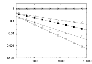
$N$

Figure 5: Error estimates (points) and the fitted convergence rates (lines) for the mass density, velocity, and $A(s)$ in the 1-D planar Noh test problem.

		$L_{1}$	$L_{2}$	$L_{\infty}$
	Std.	-0.59 $\pm$ 0.06	-0.28 $\pm$ 0.03	0.0292 $\pm$ 0.004
$\rho$	Comp.	-0.97 $\pm$ 0.01	-0.488 $\pm$ 0.002	0.001 $\pm$ 0.0001
	Std.	-0.69 $\pm$ 0.05	-0.33 $\pm$ 0.03	0.004 $\pm$ 0.0008
$v$	Comp.	-0.974 $\pm$ 0.007	-0.488 $\pm$ 0.002	0.0016 $\pm$ 0.0006
	Std.	-0.59 $\pm$ 0.06	-0.32 $\pm$ 0.03	0.008 $\pm$ 0.002
$A(s)$	Comp.	-0.985 $\pm$ 0.002	-0.487 $\pm$ 0.003	0.003 $\pm$ 0.002

Table 2: Fitted convergence rates for the mass density, velocity, and $A(s)$ in the planar Noh problem, shown $\pm 1\sigma$.

We now consider a strong shock test case, the planar Noh problem [9]. In this test case two streams of initially pressureless gas collide at the origin, setting up an infinite strength shock propagating back into the gas streams, behind which the gas is hot and motionless. We again consider a $\gamma=5/3$ gas, with initial conditions $(\rho,P,v)=(1,0,-1)$ for $x>0$ and a reflecting boundary condition at $x=0$. We run simulations with $N\in$ (25, 50, 100, 200, 400, 800, 1600, 3200, & 6400) nodes.

Figure 4 shows the profiles of the mass density, velocities, and $A(s)$ at $t=0.3$. The shock speed for our initial conditions is $v_{s}=1/3$, so the expected shock position is 0.1. The erroneous dip in the mass densities (and spike in $A(s)$) near the origin is the so called “wall heating” effect. It appears the compatible discretization has slightly less wall heating than the standard formalism (the dip in the mass density is less), as well as a smaller overshoot in $A(s)$ in this region.

Examination of the error norms in Figure 5 and the fitted convergence rates summarized in Table 2 shows that this strong shock test problem definitely benefits from the compatible discretization. The standard formalism fails to achieve first order convergence (hovering in the range $m\in[-0.6,-0.7]$), while the compatible formalism does see first order. This results in the compatible discretization achieving better accuracy for the same number of points as we increase the resolution. The critical difference between this problem and previous shock tube test case is most likely that here the energy is converted entirely from kinetic to thermal energy through the shock, while the weaker shock in the Sod test does not convert nearly as much of the energy budget in the problem between these forms. The exact energy conservation guaranteed by the compatible discretization ensures the work incurred by the accelerations due to the artificial viscosity (the dominant numerical term for this problem) is accurately represented, leading to the improved accuracy noted here. Close examination of the the profiles from all the simulations reveals that the major source of the error in the standard case is the shock position, which is slightly ahead of where it should be. This is mostly likely related to the fact that the standard form suffers a slight growth in the energy, with $\Delta E/E\sim 0.003$ at these resolutions. Although conservation to less than half a percent is typically considered quite reasonable, in this case we can measure the effects of that error in the final solution.

4.3 Cylindrical Noh shock test

In this section we look at the only multi-dimensional test considered in this paper: the cylindrical Noh problem [9] modeled in 2-D. This is largely presented as a demonstration that there is nothing special about the 1-D tests we have considered so far, and the compatibly differenced formalism works as well in multi-dimensional problems as in 1-D. The cylindrical Noh test posits that we have a cylindrically convergent flow of an initially pressureless, uniform density gas. In cylindrical coordinates $(r,\theta,z)$ the initial conditions we use can be expressed as $(\rho,P,v_{r},v_{\theta},v_{z})=(1,0,-1,0,0)$. We again use a $\gamma=5/3$ gamma-law gas, so the post-shock density should be a constant factor of 16, with the gas adiabatically compressed in the pre-shock region by a factor of 4 and then shocked an additional factor of 4 due to the shock transition. We initialize the problem with the SPH nodes on rings (with azimuthal spacing set equal to the initial radial spacing), and consider problems with the number of radial rings $N_{r}\in$ (25, 50, 100, 200, & 400).

It is worth noting that in general multi-dimensional tests such as this require the anisotropic sampling of ASPH [10] in order to achieve the expected convergence rates. However, this case is special because in 2-D the appropriate post-shock compression is in fact isotropic, so the circular shape of the 2-D SPH smoothing scale is the appropriate solution. In the pre-shock region there is anisotropic compression in the azimuthal direction, but this does not compromise the radial resolution significantly and therefore does not adversely affect the results. We do however require the tensor artificial viscosity [11] with it’s associated limiter to get reasonable results, which is why we include this term in Eqs. (2) & (3).

	$\rho$	$v_{r}$	$A(s)$
Standard
Compatible

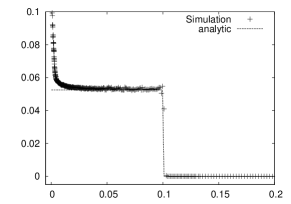
$x$

Figure 6: Radial profiles of the mass density, radial velocity, and $A(s)$ for the cylindrical Noh problem. Shown here are the results for the simulation using 400 radial rings of nodes (points) vs. the analytic solution (lines).

Examination of the profiles of the mass density, velocity, and $A(s)$ in Figure 6 shows that the compatible formalism sees slightly less wall heating and less of a corresponding spike in $A(s)$ compared with the standard results, much like in the planar Noh problem. Both methods match the pre-shock conditions quite well. However, it is evident that the compatible discretization shows improvements in the post-shock profiles, in that it more closely matches the post-shock density of 16, and $A(s)$ is closer to the analytic answer and shows less scatter. The improved post-shock density for the compatible form appears to be related to the fact that the shock position is again a little too far advanced in the run using the standard formalism. In terms of energy conservation we find that the standard form fares about as well as in the planar case, with an energy drift $\Delta E/E\sim 0.004$ (the compatible discretization maintains the expected $\Delta E/E\sim 10^{-14}$).

	$\rho$	$v_{r}$	$A(s)$
Error

$N_{r}$

Figure 7: Error estimates (points) and the fitted convergence rates (lines) for the mass density, radial velocity, and $A(s)$ in the 2-D cylindrical Noh test problem.

		$L_{1}$	$L_{2}$	$L_{\infty}$
	Std.	-0.65 $\pm$ 0.04	-0.32 $\pm$ 0.05	0.09 $\pm$ 0.02
$\rho$	Comp.	-0.894 $\pm$ 0.006	-0.498 $\pm$ 0.002	0.08 $\pm$ 0.01
	Std.	-0.73 $\pm$ 0.07	-0.34 $\pm$ 0.04	0.020 $\pm$ 0.005
$v_{r}$	Comp.	-0.90 $\pm$ 0.02	-0.490 $\pm$ 0.001	0.007 $\pm$ 0.001
	Std.	-0.77 $\pm$ 0.07	-0.54 $\pm$ 0.06	-0.04 $\pm$ 0.02
$A(s)$	Comp.	-1.00 $\pm$ 0.02	-0.57 $\pm$ 0.02	-0.17 $\pm$ 0.02

Table 3: Fitted convergence rates for the mass density, radial velocity, and $A(s)$ in the cylindrical Noh problem, shown $\pm 1\sigma$.

Examination of the measured errors and convergence rate in Figure 6 and Table 3 again mirrors what we saw in the planar Noh problem. The standard discretization does not quite make the expected first order convergence (hovering in the range $m\in[-0.65,-0.8]$), while the compatible discretization does maintain first order convergence.

4.4 Planar Taylor-Sedov blastwave test

The final test case we consider is the Taylor-Sedov blastwave [13], which is the problem of an intense explosion due to the injection of a point source of energy into an otherwise uniform, pressureless gas. This test is a useful diagnostic of how an algorithm handles relaxing extreme discontinuities in the specific thermal energy – in particular, as discussed earlier particular choices for the partitioning of the work between nodes can result in unphysically negative specific thermal energies. We model this problem in 1-D, corresponding to the planar solution in [13]. We use a $\gamma=5/3$ gamma-law gas, and consider runs using $N\in$ (51, 101, 201, 401, 801, 1601, 3201, 6401, 12801, & 25601) SPH nodes seeded in the volume $x\in[-1,1]$. Our initial conditions are $(\rho,P,v)=(1,0,0)$, and we seed an energy spike corresponding to $E_{\mbox{\scriptsize spike}}=1$ on the single point at the origin.

	$\rho$	$v$	$A(s)$
Standard
Compatible

$x$

Figure 8: Profiles of the mass density, velocity, and $A(s)$ for the planar Taylor-Sedov blastwave test case. Shown here are results from the $N=801$ node simulations (points) compared with the analytic solution (lines).

	Standard	Compatible
$\rho$

$x$

Figure 9: Zoom in on the details of the mass density profiles around the shock position in the Taylor-Sedov blastwave test case. Here we have plotted the profiles from all the resolutions ($N$ ranging from 51 to 25601) to see how the profiles are converging as compared with the analytic solution.

Figure 8 shows the profiles of the mass density, velocity, and $A(s)$ at $t$ = 0.3 for $x>0$, while Figure 9 zooms in on the mass density profiles around the shock position at this same time. It is immediately clear that in this problem the standard discretization is converging on the wrong shock position, although it is not far off. The false convergence point is just outside the expected value from the analytic solution, and the fact that the converged shock position is a bit too far out is consistent with the fact that the energy grows slightly, with $\Delta E/E\sim$ 0.1%–1%, increasing slowly with resolution. Interestingly, in running this problem we found that it was necessary to smooth the initial energy spike using a Shephard’s function formalism

$$E_{i}=\frac{E_{\mbox{\scriptsize spike}}W(x_{i}-x_{0},h_{i})}{\sum_{j}W(x_{j}-x_{0},h_{j})},$$ (22)

(where $E_{\mbox{\scriptsize spike}},x_{0}$ are the energy and position of the energy spike) in order to get either formalism to converge to the correct position. Without this smoothing, the simulated shock was too slow, and the shock position consistently lagged behind the analytic expectation. Note that this smoothing has nothing to do with avoiding negative internal energies – both formalisms used here successfully run this problem without generating any negative energies. Rather, we found this initial smoothing step necessary solely to improve the match to the position of the shock. Most likely the reason this is not typically seen in SPH simulations of this problem is due to the fact that usually those models are not run at sufficient resolution to distinguish the converged shock position as is done here. In terms of the post-shock profiles, to the eye both schemes are doing a reasonable job of capturing the post-shock shapes of the mass density, velocity, and $A(s)$. They each have some difficulty capturing the near vacuum conditions at the origin (particularly notable in $A(s)$) because this is a Lagrangian scheme, and we can only represent a solution where there is mass.

	$\rho$	$v$	$A(s)$
Error

$N$

Figure 10: Error estimates (points) and the fitted convergence rates (lines) for the mass density, velocity, and $A(s)$ in the Taylor-Sedov blastwave test problem.

		$L_{1}$	$L_{2}$	$L_{\infty}$
	Std.	-0.24 $\pm$ 0.08	-0.03 $\pm$ 0.06	0.12 $\pm$ 0.02
$\rho$	Comp.	-0.69 $\pm$ 0.04	-0.28 $\pm$ 0.04	0.10 $\pm$ 0.02
	Std.	-0.23 $\pm$ 0.06	0.04 $\pm$ 0.07	0.16 $\pm$ 0.05
$v$	Comp.	-0.62 $\pm$ 0.03	-0.18 $\pm$ 0.04	0.15 $\pm$ 0.03
	Std.	-0.4 $\pm$ 0.1	-0.3 $\pm$ 0.1	-0.2 $\pm$ 0.1
$A(s)$	Comp.	-0.80 $\pm$ 0.09	-0.6 $\pm$ 0.1	-0.2 $\pm$ 0.1

Table 4: Fitted convergence rates for the mass density, velocity, and $A(s)$ in the planar Taylor-Sedov blastwave, shown $\pm 1\sigma$.

The error norms and measured convergence rates in Figure 10 and Table 4 demonstrate the difficulty these schemes have in matching the shock position. The standard form sees quite poor convergence rates (with $m\in[-0.2,-0.4]$), while the compatible formalism sees higher convergence rates ($m\in[-0.6,-0.8]$) and corresponding more accurate solutions, but still not quite the ideal first order. If we play games such as measuring the convergence by normalizing the positions of the profiles to the measured shock position and compare to a normalized analytic answer, our measured errors improve substantially and we see convergence at first order for both schemes. It is debatable whether it is more appropriate to fudge the error measurements in this manner or not, but for this work we have elected to simply measure the errors against the exact solution including the shock position, since this is after all what we would be looking for were we modeling this problem without access to the analytic solution.

5 Conclusions

We have derived a total energy conserving form of SPH based on the compatible differencing ideas described in [2]. The compatible formalism guarantees energy conservation by exactly accounting for the work done by the discrete pair-wise accelerations between SPH nodes. We describe a scheme for dividing the pair-wise work between points such that the work term will tend to drive the temperatures of the points closer to one and other, avoiding the introduction of new extrema in the thermal energy (such as unphysical negative temperature excursions). This new scheme should represent a very minor modification for existing SPH codes; indeed, as demonstrated in §3.1.1 the algorithm described here is very closely related to the standard discretizations of the energy equation.

We have demonstrated through a series of tests that the compatible energy discretization for SPH results in quantifiable improvements in the accuracy and convergence properties of the algorithm. In order to address the natural concern over the accuracy of the entropy solution in an energy conserving scheme such as ours, we have explicitly investigated the accuracy of the entropy evolution by examining the behaviour of the entropic function $A(s)=P/\rho^{\gamma}$ in our tests, comparing the simulations to analytic solutions. In all cases the accuracy of the entropy evolution has been improved by use of the compatible discretization. At first this might seem odd to someone accustomed to seeing larger entropy errors in energy conserving schemes. The explanation comes from considering the differences in the approach taken here: in this case we are still evolving the internal energy, we are simply making a more accurate accounting of the discrete work done by the numerically estimated accelerations. Often energy conservation is achieved by evolving the total energy and deriving the thermal energy by taking the difference between the total and kinetic energies, which can squeeze the discretization errors into the thermal term (particularly in strongly supersonic flows). We view the changes proposed here as more akin to the difference between updating the mass density according the SPH sum (such as Eq. 1) vs. time evolving the continuity equation. In general using the sum definition for the density is more accurate, because we have removed a source of error by not time evolving the total mass in some sense. There are times when evolving the continuity equation makes more sense (such as solids with equations of state that are not forgiving of the surface problems with Eq. 1), but in fluid problems where the sum definition for the mass density is reasonable, it will generally prove more accurate. We believe this is analogous to the changes we have proposed here. By exactly accounting for the numerical work done by the momentum equation (Eq. 2), we have removed one of the components of error (a time evolved definition of the energy) rather than just force the discretization errors into the thermal energy equation.

We should also point out that we do not mean to suggest that the accuracy improvements in the SPH discretization possible by accounting for the variable $h$ terms such as described in [15] and [12] should be neglected. These authors find that the fundamental accuracy of the numerics is improved when self-consistently accounting for the effects of allowing a variable smoothing scale, which also has the effect of improving the energy conservation. This improved energy conservation is simply a reflection of the fact that the authors are achieving a more accurate solution of the problem for some additional computational cost. We would propose that one could see even greater benefit by combining these approaches – there is no reason one cannot use the compatible energy formalism described in this paper on top of a scheme which also accounts for the effects of the variable $h$. Indeed, one nice aspect of the compatible formalism is that it can be used on top of any scheme for computing the pair-wise accelerations $a_{ij}$ – it does not really matter how you arrived at the acceleration, only that you then self-consistently account for the discrete work done by those accelerations. Additionally, one can compatibly introduce the work done by any physics that creates an acceleration on the SPH points in a similar manner. In this way the compatible discretization actually improves on the simplicity of adding new physics to an SPH scheme.

There are however computational expense tradeoffs to be made. We find that by spending memory to hold the pair-wise accelerations for each interacting pair of nodes that the computational run-time for a typical problem is only increased by a few percent in our implementation. However, the required memory use may not be practical on all computer architectures, in which case it will be necessary to compute the pair-wise accelerations twice, most likely resulting in a larger run-time penalty than we see here.

We believe that the improvements demonstrated here are relevant for typical SPH applications, such as modeling galaxy formation. For instance, the important physical process in the Noh problem (§4.2 & 4.3) is the conversion of the kinetic energy due to a convergent inflow to thermal energy via a strong shock – this mirrors one of the dominant processes in the formation of galaxies and galaxy clusters, where the kinetic energy due to the gravitational infall of the gas is converted almost entirely to thermal energy through strong shocks. The Taylor-Sedov blastwave (§4.4) consists of the introduction of a strong thermal energy source into an ambient gas, much like the way the process of star formation in SPH modeling of galactic evolution introduces thermal energy released by the absorption of radiation from hot young stars and supernovae back into the simulated interstellar medium. There is a potential lesson for such models though in the fact that we still found it beneficial (in terms of the accuracy of the final solution) to smooth the initial energy deposition in the Taylor-Sedov problem. This issue may warrant further investigation.

JMO would like to acknowledge many valuable discussions with Doug Miller. We would also like to acknowledge some useful suggestions from the referees which have contributed to the clarity of this manuscript. This work was performed under the auspices of the U.S. Department of Energy by the University of California, Lawrence Livermore National Laboratory under contract No. W-7405-Eng-48.

References

- [1] W. Benz, in “The Numerical Modeling of Nonlinear Stellar Pulsations,” (Boston: Kluwer), 269 (1990)
- [2] E. J. Caramana, D. E. Burton, M. J. Shashkov, and P. P. Whalen, J. Comp. Phys., 146, 227 (1998)
- [3] R. A. Gingold and J. J. Monaghan, MNRAS, 181, 375 (1977)
- [4] L. Hernquist, Astrophys. J., 404, 717 (1993)
- [5] L. B. Lucy, Astron. J., 82, 1013 (1977)
- [6] J. J. Monaghan, Ann. Rev. Astron. & Astrophys., 30, 543 (1992)
- [7] J. J. Monaghan and R. A. Gingold, J. Comp. Phys., 52, 374 (1983)
- [8] R. P. Nelson and J. C. B. Papaloizou, MNRAS, 270, 1 (1994)
- [9] W. F. Noh, J. Comp. Phys., 72, 78 (1987)
- [10] J. M. Owen, J. V. Villumsen, P. R. Shapiro, and H. Martel, Astrophys. J. Supp., 116, 155 (1998)
- [11] J. M. Owen, J. Comp. Phys., 201, 601 (2004)
- [12] D. J. Price and J. J. Monaghan, MNRAS, accepted.
- [13] L. I. Sedov, in “Similarity and Dimensional Methods in Mechanics,” (New York: Academic Press Inc.), 210 (1959)
- [14] G. A. Sod, J. Comp. Phys., 27, 1 (1978)
- [15] V. Springel and L. Hernquist, MNRAS, 333, 649 (2002)
- [16] V. Springel and L. Hernquist, Astrophys. J., 622, L9 (2004)
- [17] R. J. Thackar, E. R. Tittley, F. R. Pearce, H. M. P. Couchman, and P. A. Thomas, MNRAS, 319, 619 (2000)