The spatial string tension in the deconfined phase of three dimensional QCD in the large N limit
Abstract:
We numerically compute the spatial string tension in the deconfined phase of three dimensional QCD in the large N limit. Our results clearly show that the string tension grows linearly with temperature.
Three dimensional QCD on a symmetric torus is considered in the large N limit. This theory is known to be in the deconfined phase for [1]. is the temperature at which one of the three symmetries is broken and is the temperature at which two of the three symmetries are broken111 can be taken to infinity by working on an asymmetric torus with one short (temperature) direction and two long (spatial) directions..
At leading order in , the string tension is independent of the temperature in the confined phase (), and it was computed using reduction [2]. Since the symmetry is broken only in one direction in the deconfined phase, spatial Wilson loops in the plane perpendicular to the broken direction are expected to show confining behavior. This has been numerically observed in the deconfined phase of SU(2) Yang-Mills theory in four dimensions [3].
We use the standard Wilson gauge action,
| (1) |
on a lattice with periodic boundary conditions. The ’t Hooft limit is obtained by keeping the coupling fixed as we take . We use the tadpole improved lattice coupling [4],
| (2) |
instead of the lattice coupling . We approach the continuum limit in the deconfined phase by taking and keeping the physical temperature, fixed. The upper and lower limits of the deconfined phase have been numerical estimated [1] to be
| (3) | |||||
| (4) |
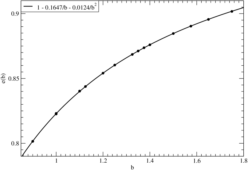
We used and to extract the behavior of the string tension as a function of the temperature in the deconfined phase. We also used and to verify that was large enough for us to ignore finite effects. The complete list of couplings used in the numerical analysis can be found in Table 1, and the full range from and has been covered. A plot of the average energy listed in Table 1 is plotted in Figure 1 along with a fit that includes a and a term. The tadpole improved coupling removes some large lattice spacing effects that are common to all observables.
We used an order parameter based on the Polyakov loop and defined by [5]
| (5) | |||||
| (6) | |||||
| (7) |
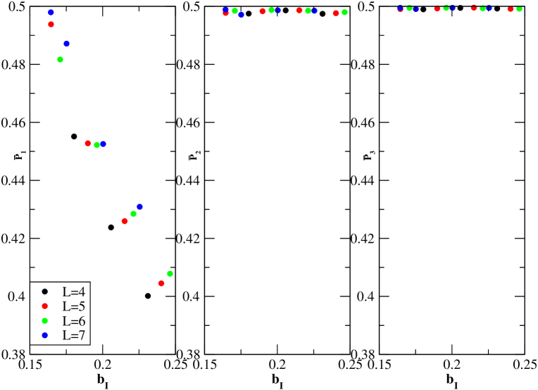
to ensure that we are in the deconfined phase. The quantity takes values in the range on any gauge field background, and we choose the directions such that such that . The deconfined phase corresponds to and within errors. The data presented in Table 1 and plotted in Figure 2 shows this to be the case.
We use computational techniques identical to the ones described in [2] to compute the static potential in the deconfined phase of large N QCD for spatial Wilson loops. As discussed in [2], our links in the plane are smeared while the links in direction are not smeared. We have set the smearing factor to and the number of smearing steps to . We compute the expectation values of all loops, , in the (spatial) plane with . Keeping fixed, we fit
| (8) |
Since becomes small as becomes big, we do not use all values of for the fit. The range of is determined such that the relative error of the fit per degree of freedom (number of values of used in the fit) is less than , and this typically included all loops with . The static potential is subsequently fit to
| (9) |
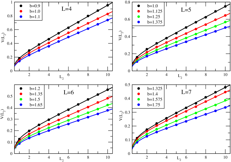
The results for , and are shown in Table 1. The performance of the fits for at can be seen in the plots of the static potential in Figure 3. A comparison of the values of for and at for the three different values of shows that finite effects are small at .
The last column in Table 1 provides all the results obtained in this paper for the spatial string tension at several values of the temperature in the deconfined phase. If we use high temperature dimensional reduction similar to the arguments in [3], the effective two dimensional coupling is
| (10) |
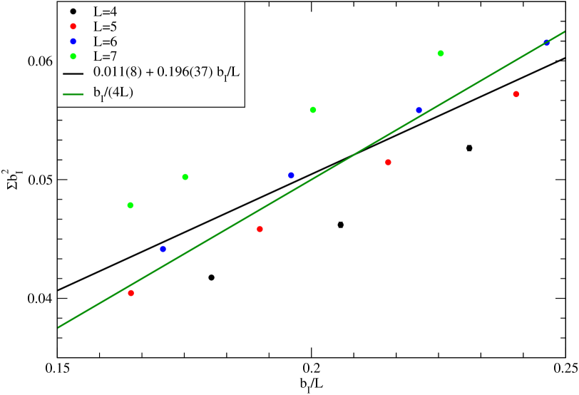
If the spatial string tension in the deconfined phase is equal to the string tension in the two dimensional theory, then we expect [6]
| (11) |
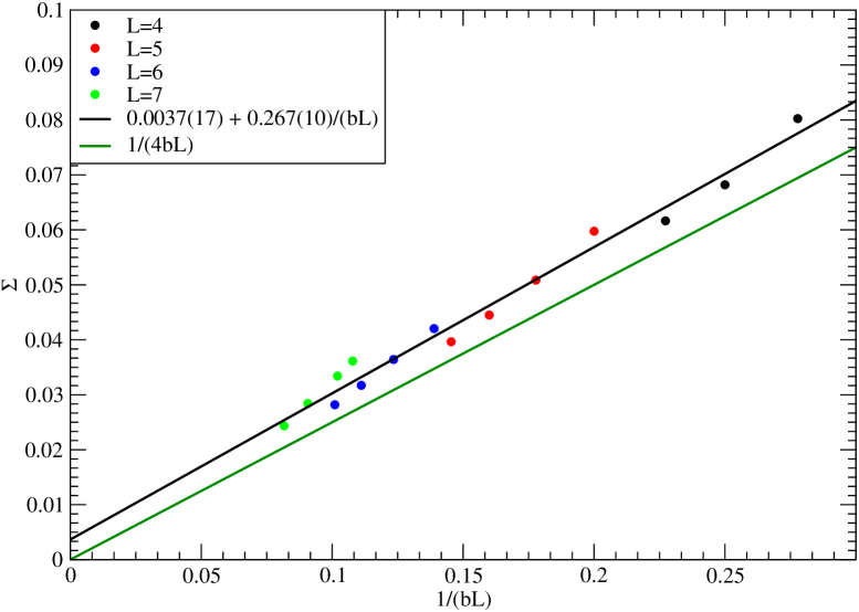
A plot of versus is shown in Figure 4. The combined data at the four different values of are fit to a straight line. Considering that the value of is modest and that its value is not large, the fit is surprisingly consistent with the prediction in (11).
Another way to plot Figure 4 is to convert the axes to physical units (physical string tension vs. physical temperature) and use tadpole improved coupling. Such a plot is shown in Figure 5. At the same physical , larger corresponds to finer lattice spacing. Thus finite spacing effects appear as the scatter in in this plot, and the fit coefficients are slightly different from those in Figure 4.
If we assume (11) to be valid in the entire region of the deconfined phase and use [7] for the string tension in the confined phase, continuity of the string tension across the phase transition suggests that consistent with (4).
Alternatively, we can compare the results here and in [2]. When the measured values for at are extrapolated to we obtain 0.232(11), which compares favorably with the corresponding value in Table 1.
If the spatial string tension is indeed continuous at , then we have a picture for the limit in which the spatial and temporal string tensions are equal and independent of for . At , the temporal string tension falls to zero discontinuously, and the spatial string tension begins to grow linearly with .
Acknowledgments.
R.N. acknowledges partial support by the NSF under grant number PHY-055375.References
- [1] R. Narayanan, H. Neuberger and F. Reynoso, Phys. Lett. B 651, 246 (2007) [arXiv:0704.2591 [hep-lat]].
- [2] J. Kiskis and R. Narayanan, JHEP 0809, 080 (2008) [arXiv:0807.1315 [hep-th]].
- [3] G. S. Bali, J. Fingberg, U. M. Heller, F. Karsch and K. Schilling, Phys. Rev. Lett. 71, 3059 (1993) [arXiv:hep-lat/9306024].
- [4] G. P. Lepage, arXiv:hep-lat/9607076.
- [5] G. Bhanot, U. M. Heller and H. Neuberger, Phys. Lett. B 113, 47 (1982).
- [6] D. J. Gross and E. Witten, Phys. Rev. D 21, 446 (1980).
- [7] D. Karabali, C. j. Kim and V. P. Nair, Phys. Lett. B 434, 103 (1998) [arXiv:hep-th/9804132].