A study of the Galactic plane towards $l=305^{\circ}$

Abstract

We present optical ($UBVI_{C}$) observations of a rich and complex field in the Galactic plane towards $l\sim 305^{\circ}$ and $b\sim 0^{\circ}$. Our analysis reveals a significantly high interstellar absorbtion ($A_{V}\sim 10$) and an abnormal extinction law in this line of sight. Availing a considerable number of color combinations, the photometric diagrams allow us to derive new estimates of the fundamental parameters of the two open clusters Danks 1 and Danks 2. Due to the derived abnormal reddening law in this line of sight, both clusters appear much closer (to the Sun) than previously thought. Additionally, we present the optical colors and magnitudes of the WR 48a star and its main parameters were estimated. The properties of the two embedded clusters DBS2003 130 and 131, are also addressed. We identify a number of Young Stellar Objects which are probable members of these clusters. This new material is then used to revisit the spiral structure in this sector of the Galaxy showing evidence of populations associated with the inner Galaxy Scutum-Crux arm.

Galactic plane at $l=305^{\circ}$

1 Introduction

The study of embedded Galactic clusters is fundamental in tracing the Galactic spiral structure and improve our understanding of the star formation process. Our group has investigated several Galactic plane regions in the fourth quadrant line of sights (see Vázquez et al. 2005, Carraro & Costa 2009), and in this paper we further extend this study to a region located at $l=305^{\circ}$ and $b\sim 0^{\circ}$. This region contains very interesting objects; being an important cloud which obscure two compact young open clusters (Danks 1 and Danks 2), a WR star (WR 48a), and at least three embedded clusters (DBS2003 130, 131 and 132) so far detected only in the infrared (Dutra et al. 2003). There are also several HII regions and OH/H₂O maser sources (see Danks et al. 1984 or Clark & Porter 2004 for a detailed description).

The open clusters Danks 1 and Danks 2 were first detected by Danks et al. (1983) and their parameters were only recently estimated by Bica et al. (2004), using $BVI$ and $JHK$ photometry. In this regards, we show that complementing the optical and infrared data with $U$ observations adds valuable information that allow a better determination of the interstellar absorption in this line of sight. As for the embedded clusters, it is important to note that only DBS2003 131 has been extnsively studied in the infrared (Leistra et al. 2005 and Longmore et al. 2007), and that none of 3 clusters has been studied in the optical.

In the present paper we perform a detailed wide field study at $l=305^{\circ}$ using all $UBVI$ and $JHK$, of all the aforementioned objects, and derive updated estimates of their fundamental parameters. We then analyze this field with respect to other fields in the fourth Galactic quadrant to derive information about the Galactic spiral structure of this portion of the disk.

The layout of the paper is as follows. In Sect. 2 we describe the used data, and the reduction and calibration procedures. In Sect. 3 we present the analysis of the data together with the main clusters parameters. Finally, in Sects. 4 and 5 we discuss and summarize our results.

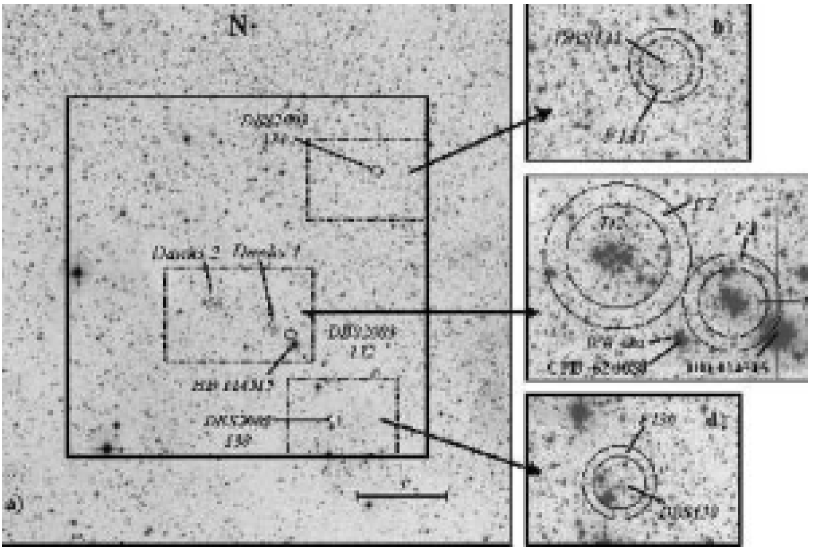
Figure 1: Left image (panel a) shows a second generation Digitized Sky Survey (DSS-2; red filter) image centered at $\alpha_{2000}=13:12:43.4$; $\delta_{2000}=-62:39:2.2$ and covering a field of $30\aas@@fstack{\prime}0\times 30\aas@@fstack{\prime}0$. Open clusters Danks 1/2; embedded clusters DBS2003 130, 131 and 132; and HD 1145115 star are identified. Solid square indicates the full studied area whereas the dotted rectangles trace the regions highlighted in the right minor panels (b, c and d), as these appear on our long $I$ exposure.

2 Data

2.1 Observations

$UBVI_{C}$ images of the region under study (see Fig. 1) were acquired using the Y4KCAM camera attached to the 1.0m telescope, which is operated by the SMARTS consortium and placed at Cerro Tololo Inter-American Observatory (CTIO). This camera is equipped with an STA $4064\times 4064$ CCD with $15\mu$ pixels. This set-up provides direct imaging over a field of view (FOV) $20\aas@@fstack{\prime}0\times 20\aas@@fstack{\prime}0$ with a scale of $0\aas@@fstack{\prime\prime}289$/pix. The relatively large FOV allowed us to include several objects present in the region and also to have an important sample of the adjacent stellar field in this part of the Galactic plane. The CCD was operated without binning, at a nominal gain and read out noise of 1.44 e-/ADU and 7 e- per quadrant (this detector is read by means of four different amplifiers). Other detector characteristics can be found at http://www.astronomy.ohio-state.edu/Y4KCam/detector.html. Details on the observations are given in Table LABEL:tab:frames. Typical FWHM of the data was about $0\aas@@fstack{\prime\prime}9$ and airmasses values during the observation of the scientific frames ranged 1.19-1.22.

Table 1: Journal of observations of the scientific frames together with used calibration coefficients (23-24 March 2006).

Exposure times [sec]x$N$
Date	Frames	$U$	$B$	$V$	$I_{C}$	$N_{f}$
Scientific frames
23-24	long	2000x5	1200x2	900x2	700x2	1
	medium	200x2	100x2	100x2	100x2	1
	short	30x2	30x2	30x2	30x2	1
Standard frames (Landolt 1992)
23	SA101	400	200	150	130	2
	SA107	200	50	30	30	3
24	SA101	400	200	150	130	2
	SA101	200	50	30	30	1
	SA104	400	200	150	130	1
	SA104	200	50	30	30	1
	SA107	200	50	30	30	3
Calibration and extinction coefficients
$u_{1}=+3.284\pm 0.007$			$v_{1bv}=+1.822\pm 0.010$
$u_{2}=-0.025\pm 0.012$			$v_{2bv}=-0.054\pm 0.012$
$u_{3}=+0.45$			$v_{1vi}=+1.836\pm 0.008$
$b_{1}=+2.025\pm 0.012$			$v_{2vi}=-0.059\pm 0.009$
$b_{2}=+0.167\pm 0.015$			$v_{3}=+0.16$
$b_{3}=+0.25$			$i_{1}=+2.677\pm 0.016$
			$i_{2}=-0.002\pm 0.018$
			$i_{3}=+0.08$

Notes: $N$ indicates the number of obtained exposures in case it is more than 1, while $N_{f}$ indicates the amount of different observed frames in each field.

2.2 Reduction

All frames were pre-processed in a standard way using the IRAF package CCDRED. To this aim, zero exposures and sky flats were taken every night. In order to achieve deep photometry, all the long exposures within each band were combined using IMCOMBINE task. This procedure helps to remove cosmic rays and improve the signal-to-noise ratio of the faintest stars. In particular, five images were combined in $U$ band, allowing us to reach the $U-B$ index for the brightest stars of Danks 1 and Danks 2. However it was not enough for the case of embedded clusters, were only data in $BVI$ bands could be obtained.

Photometry was then performed using IRAF DAOPHOT and PHOTCAL packages. Instrumental magnitudes were obtained using the point spread function (PSF) method (Stetson 1987). Since the FOV is large, a quadratic spatially variable PSF was adopted and its calibration on each image was done using several isolated, spatially well distributed, bright stars (about 25) across the field. The PSF photometry was finally aperture-corrected for each filter and exposure time. Aperture corrections were computed performing aperture photometry of a suitable number (about 20) of bright stars in the field. In order to obtain a more complete sample of the stars in the observed region, an additional photometry table was generated using as input the coordinates (converted to pixels) of all the stars that according to the 2MASS catalogue must be present in our FOV. Finally, all data from different filters and exposures were combined and calibrated using DAOMASTER (Stetson 1992).

2.3 Photometric calibration

Standard star selected areas (see Table LABEL:tab:frames) from the catalog of Landolt (1992) were used to determine the transformation equations relating our instrumental magnitudes to the standard $UBVI_{C}$ system. The selection of the fields was done in order to provide a wide range in colors. Then, aperture photometry was carried out for all the standard stars ($\sim 70$ per night) using the IRAF PHOTCAL package. To tie our observations to the standard system, we use transformation equations of the form:

$u=U+u_{1}+u_{2}(U-B)+u_{3}X$	($r.m.s.=0.04$)	(1)
$b=B+b_{1}+b_{2}(B-V)+b_{3}X$	($r.m.s.=0.03$)	(2)
$v=V+v_{1bv}+v_{2bv}(B-V)+v_{3}X$	($r.m.s.=0.02$)	(3)
$v=V+v_{1vi}+v_{2vi}(V-I_{C})+v_{3}X$	($r.m.s.=0.02$)	(4)
$i=I_{C}+i_{1}+i_{2}(V-I_{C})+i_{3}X$	($r.m.s.=0.02$)	(5)

where $UBVI_{C}$ and $ubvi$ are standard and instrumental magnitudes respectively and $X$ is the airmass of the observation. The transformation coefficients and extinction coefficients for the CTIO Observatory are shown at the bottom of Table 1. To derive $V$ magnitudes, we use expression (3) when the $B$ magnitude was available; otherwise expression (4) was used.

2.4 Complementary data and astrometry

Other available catalogues, such as the Two-Micron All Sky Survey (2MASS; Cutri et al. 2003, Skrutskie et al. 2006) are of fundamental importance to perform a more complete analysis of the region under investigation. Therefore, using the X–Y stellar positions obtained from our data, their equatorial coordinates were computed. First of all, a matched list of X–Y and RA, DEC was built by visually identifying about 20 2MASS stars in the field under study. The stars in the list were then used to obtain transformation equations to get equatorial coordinates for the remaining stars. In a second step, a computer routine was used to cross-identify all the sources in common with the same catalogues by matching the equatorial coordinates to the catalogued ones. The rms of the residuals were $\sim 0\aas@@fstack{\prime\prime}17$, which is about the astrometric precision of the 2MASS catalogue ($\sim 0\aas@@fstack{\prime\prime}12$), as expected since most of the coordinates were retrieved from this catalogue.

2.5 Final catalogue

The above procedure allowed us to build an astrometric, photometric ($UBVIJHK$) catalogue that constitutes the main observational database used in this study. A solid analysis of the behavior of the Stellar Energy Distributions (SEDs) can be carried out with this tool, thus preventing possible degeneracies in the photometric diagrams and allowing to obtain more reliable results. The full catalogue with a total of 34310 stars is only available in electronic form at the Centre de Donnes astronomiques de Strasbourg (CDS). It includes X–Y positions; 2MASS identification (when available); equatorial coordinates (epoch 2000.0); optical and 2MASS photometry. Table 2 is a summary of that catalogue including only stars adopted as likely cluster members or probable young stellar objects (YSOs).

Table 2: A sample of the final catalogue used in this study.

ID	2MASS ID	$X[pix]$	$Y[pix]$	$\alpha_{J2000}$	$\delta_{J2000}$	$V$	$B$-$V$	$U$-$B$	$V$-$I$	$K$	$J$-$H$	$H$-$K$	Comments
256	J13122855-6241438	1662.1	2563.4	13:12:28.6	-62:41:43.4	14.964	2.448	1.389	3.720	6.610	0.989	0.656	D1	lm
659	J13122850-6241509	1660.7	2587.8	13:12:28.5	-62:41:50.5	16.214	2.417	1.426	3.854	8.150	0.979	0.684	D1	lm
733	J13122626-6242095	1607.8	2652.7	13:12:26.3	-62:42:09.2	16.359	2.466	1.283	3.679	8.507	0.906	0.499	D1	lm
1124	J13122617-6241576	1605.9	2611.5	13:12:26.2	-62:41:57.3	16.954	2.744	1.349	4.028	7.756	1.294	0.560	D1	lm
1527	J13122369-6242013	1546.9	2623.8	13:12:23.8	-62:42:00.8	17.355	2.771	1.772	4.519	7.531	1.218	0.665	D1	lm
1578	J13122497-6242002	1576.7	2619.6	13:12:25.0	-62:41:59.6	17.401	2.622	1.819	4.520	7.477	1.276	0.669	D1	lm
2683	J13122678-6241571	1621.4	2607.2	13:12:26.9	-62:41:56.0	18.160	2.406	1.905	4.019	8.135	2.076	0.566	D1	lm
2819	J13123412-6241359	1793.8	2535.6	13:12:34.1	-62:41:35.4	18.228	2.108	1.296	3.551	10.798	0.878	0.418	D1	lm
2861	–	1650.6	2551.2	13:12:28.1	-62:41:39.9	18.251	2.219	1.140	3.559	–	–	–	D1	lm
3335	J13122721-6242041	1630.7	2633.8	13:12:27.3	-62:42:03.7	18.480	2.157	1.604	3.795	10.046	1.058	0.637	D1	lm
3505	–	1601.0	2609.4	13:12:26.0	-62:41:56.6	18.562	2.091	1.942	3.891	–	–	–	D1	lm
3518	–	1670.5	2579.6	13:12:28.9	-62:41:48.1	18.568	2.184	1.542	3.691	–	–	–	D1	lm
3694	J13122288-6241488	1527.4	2580.8	13:12:22.9	-62:41:48.4	18.644	2.256	1.818	4.196	9.644	1.057	0.571	D1	lm
3921	J13122693-6242147	1624.0	2669.3	13:12:27.0	-62:42:14.0	18.737	2.129	1.515	3.811	10.296	0.856	0.685	D1	lm
4046	–	1608.4	2605.5	13:12:26.3	-62:41:55.5	18.780	2.380	1.763	4.019	–	–	–	D1	lm
4122	J13122705-6242079	1626.3	2646.4	13:12:27.1	-62:42:07.3	18.806	2.098	1.350	3.544	9.770	0.861	1.888	D1	lm
4168	J13122525-6241555	1585.2	2605.3	13:12:25.4	-62:41:55.5	18.826	2.155	1.894	3.837	8.904	2.692	0.338	D1	lm
4502	J13122959-6241291	1685.7	2512.4	13:12:29.6	-62:41:28.7	18.938	2.112	1.950	3.683	11.069	0.944	0.458	D1	lm
4664	–	1610.3	2639.3	13:12:26.4	-62:42:05.3	18.990	2.106	1.486	3.587	–	–	–	D1	lm
5245	–	1624.6	2633.6	13:12:27.0	-62:42:03.7	19.207	2.293	1.917	3.682	–	–	–	D1	lm
5557	–	1602.8	2621.1	13:12:26.1	-62:42:00.0	19.304	2.333	1.723	3.848	–	–	–	D1	lm
5569	J13123061-6242081	1710.3	2647.6	13:12:30.6	-62:42:07.7	19.309	2.326	2.661	4.129	10.222	1.118	0.616	D1	lm
5833	J13122454-6242088	1565.7	2649.8	13:12:24.5	-62:42:08.3	19.391	2.136	2.106	4.089	10.433	1.103	0.565	D1	lm
6519	J13122498-6241456	1577.3	2568.3	13:12:25.0	-62:41:44.8	19.589	2.278	1.565	3.799	11.286	0.950	0.594	D1	lm
223	J13125643-6240283	2325.1	2300.8	13:12:56.4	-62:40:27.8	14.793	2.386	1.617	3.547	6.873	0.896	0.527	D2	lm
264	J13124634-6241262	2085.4	2501.7	13:12:46.3	-62:41:25.7	14.999	2.324	1.272	3.406	7.792	0.818	0.425	D2	lm
287	J13124958-6241207	2162.7	2482.7	13:12:49.6	-62:41:20.3	15.095	2.120	1.051	3.127	8.595	0.686	0.400	D2	lm
775	J13125627-6240515	2321.6	2381.5	13:12:56.2	-62:40:51.1	16.409	2.343	1.105	3.489	9.306	0.770	0.402	D2	lm
892	J13125456-6241050	2280.9	2428.3	13:12:54.5	-62:41:04.6	16.618	2.343	1.057	3.388	9.654	0.779	0.369	D2	lm
936	J13125236-6240463	2228.5	2363.6	13:12:52.3	-62:40:45.9	16.672	2.159	1.070	3.205	10.059	0.725	0.369	D2	lm
979	J13125864-6240552	2378.1	2394.4	13:12:58.6	-62:40:54.9	16.728	2.349	1.059	3.491	9.556	0.803	0.396	D2	lm
989	J13125396-6240475	2266.4	2367.6	13:12:53.9	-62:40:47.1	16.741	2.196	1.056	3.209	10.104	0.731	0.334	D2	lm
1026	J13125445-6240459	2278.0	2362.3	13:12:54.4	-62:40:45.5	16.795	2.273	0.907	3.291	9.920	0.802	0.416	D2	lm
1260	J13125829-6240371	2369.8	2331.4	13:12:58.3	-62:40:36.7	17.098	2.340	1.154	3.611	9.628	0.820	0.413	D2	lm
1409	J13125325-6240346	2249.7	2323.0	13:12:53.2	-62:40:34.2	17.247	2.076	0.945	3.343	10.529	0.735	0.342	D2	lm
1577	J13124747-6240547	2112.2	2392.4	13:12:47.5	-62:40:54.2	17.399	2.163	0.898	3.271	10.725	0.756	0.326	D2	lm
1608	J13125436-6240422	2276.1	2349.2	13:12:54.3	-62:40:41.8	17.428	2.219	1.080	3.354	10.529	0.763	0.359	D2	lm
1631	J13125731-6240268	2346.2	2296.5	13:12:57.3	-62:40:26.6	17.453	2.327	1.048	3.582	8.504	1.789	0.836	D2	lm
1671	J13125373-6240508	2261.3	2379.1	13:12:53.7	-62:40:50.4	17.489	2.230	1.017	3.376	10.477	0.779	0.363	D2	lm
1704	J13125356-6240119	2257.1	2243.9	13:12:53.6	-62:40:11.4	17.513	2.355	1.254	3.725	9.891	0.854	0.413	D2	lm
1792	J13125529-6240416	2297.7	2346.7	13:12:55.3	-62:40:41.0	17.580	2.382	0.840	3.302	10.307	0.745	0.439	D2	lm
2248	J13130084-6239545	2430.5	2183.7	13:13:00.8	-62:39:54.0	17.918	2.134	1.356	3.287	11.229	0.777	0.308	D2	lm
2272	J13125269-6240545	2236.6	2391.7	13:12:52.7	-62:40:54.0	17.931	2.132	1.014	3.217	11.293	0.728	0.309	D2	lm
2500	J13125226-6240242	2226.0	2286.5	13:12:52.2	-62:40:23.6	18.073	2.115	1.056	3.379	11.066	0.766	0.394	D2	lm
2533	J13125193-6240579	2218.5	2403.7	13:12:51.9	-62:40:57.5	18.091	2.110	1.165	3.377	11.107	0.784	0.373	D2	lm
2700	J13125237-6240314	2229.1	2311.9	13:12:52.4	-62:40:31.0	18.168	2.071	1.086	3.279	11.344	0.741	0.404	D2	lm
3215	J13124526-6240421	2059.3	2349.1	13:12:45.3	-62:40:41.7	18.426	2.042	2.545	3.291	11.079	1.139	0.376	D2	lm
3388	J13125828-6240526	2369.5	2385.1	13:12:58.3	-62:40:52.2	18.506	2.031	1.354	3.370	11.505	0.793	0.340	D2	lm
3199	J13115353-6246577	829.8	3652.4	13:11:53.6	-62:46:57.5	18.420	1.874	1.475	2.775	11.702	0.976	0.704	D130	yso?
3486	J13115601-6247114	889.3	3700.3	13:11:56.1	-62:47:11.4	18.554	2.062	3.299	2.974	11.787	1.035	0.473	D130	yso?
3624	J13115851-6247072	948.6	3685.4	13:11:58.6	-62:47:07.1	18.617	1.962	2.159	3.004	11.700	1.087	0.407	D130	yso?
9376	J13115519-6247072	870.8	3685.7	13:11:55.4	-62:47:07.2	20.249	2.111	2.696	3.310	12.308	1.392	-0.259	D130	yso?
12300	J13115237-6246517	801.3	3633.2	13:11:52.5	-62:46:52.0	20.720	2.146	0.021	2.607	13.956	1.009	1.021	D130	yso?
13396	–	774.4	3636.3	13:11:51.3	-62:46:52.9	20.889	1.991	1.244	2.669	–	–	–	D130	yso?
7046	–	439.8	785.8	13:11:37.4	-62:33:09.7	19.737	2.531	3.769	4.343	–	–	–	D131	yso?
9892	–	479.9	800.9	13:11:39.1	-62:33:14.1	20.337	3.125	1.362	5.469	–	–	–	D131	yso?
12192	–	406.2	798.5	13:11:36.0	-62:33:13.4	20.704	2.326	–	4.493	–	–	–	D131	yso?
13636	–	450.4	800.1	13:11:37.9	-62:33:13.8	20.924	6.467	–	3.997	–	–	–	D131	yso?
14868	J13114106-6232570	525.7	741.5	13:11:41.1	-62:32:57.0	21.107	2.553	-0.300	5.166	9.575	1.366	0.819	D131	yso?-A1
15897	–	520.6	741.9	13:11:40.8	-62:32:57.1	21.247	–	–	5.334	–	–	–	D131	yso?
16128	–	622.8	805.9	13:11:45.1	-62:33:15.6	21.277	2.664	1.699	5.888	–	–	–	D131	yso?
16664	–	347.5	847.0	13:11:33.6	-62:33:27.3	21.351	2.534	-0.207	5.002	–	–	–	D131	yso?-A2
18863	–	534.4	812.4	13:11:41.4	-62:33:17.4	21.632	2.821	0.596	4.837	–	–	–	D131	yso?-CO
21172	J13113947-6233283	487.9	850.0	13:11:39.5	-62:33:28.3	21.899	2.503	1.490	4.886	11.939	1.471	0.657	D131	yso?-A3
22042	–	417.2	791.1	13:11:36.5	-62:33:11.2	22.003	–	–	4.420	–	–	–	D131	yso?
25701	–	495.4	777.4	13:11:39.8	-62:33:07.3	22.452	2.685	0.942	4.791	–	–	–	D131	yso?
26479	–	496.5	818.1	13:11:39.8	-62:33:19.0	22.556	–	–	5.027	–	–	–	D131	yso?
28362	–	477.7	839.5	13:11:39.0	-62:33:25.2	22.873	2.629	–	5.341	–	–	–	D131	yso?
30644	J13113382-6233270	354.0	847.7	13:11:33.8	-62:33:27.5	23.475	–	–	3.694	10.342	1.308	0.678	D131	yso?

Note 1: Comments column indicate the star region location and its adopted membership. (D1/2 = Danks 1/2 regions; D130/131 = DBS130/131 regions; lm = likely member; yso? = probable YSO; A1, A2, A3 and CO are identifications from Leistra et al. 2005)

Note 2: A full version of this table is only available in electronic form at the Centre de Donnes astronomiques de Strasbourg (CDS).

3 Data analysis

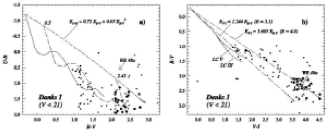
Figure 2: Optical TCDs of stars located in $D1$ zone. See also Sect 3.1 and Fig. 1 for zone definitions. a) $U-B$ vs. $B-V$ diagram. Heavy black circles are likely cluster members whereas light dots are likely field stars. The solid line is the Schmidt-Kaler (1982) ZAMS, while dashed lines are the same ZAMS, but shifted along the reddening line by the adopted color excesses indicated above them. They correspond to the adopted ones for the foreground population ($E_{B-V}=0.5$) and for the cluster stars ($E_{B-V}=2.45$). See also Sect. 3.3. The dashed arrow indicates the normal reddening path. b) $B-V$ vs. $V-I$ diagrams. Symbols are the same as in panel a) and solid lines are intrinsic colors for luminosity class V and III from Cousins (1978ab). Dashed arrows indicate the reddening paths for normal ($R_{V}=3.1$) and abnormal $R_{V}$ values.

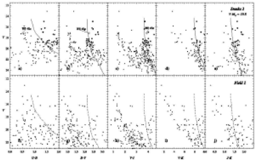
Figure 3: Optical CMDs of stars located in $D1$ and $F1$ zones. See also Sect  3.1 and Fig 1 for zone definitions. Symbols are the same as in Fig 2. The solid and dashed curves are the Schmidt-Kaler (1982) empirical ZAMS and the MS path from Cousins (1978ab) and Koornneef (1983). Solid curves are corrected by the adopted cluster apparent distance modulus (see Sect. 3.3).

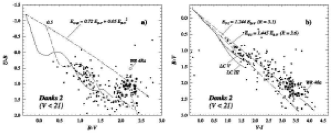
Figure 4: Optical TCDs of stars located in $D2$ zones. See also Sect 3.1 and Fig. 1 for zone definitions. Symbols and curves are teh same as in Fig. 2

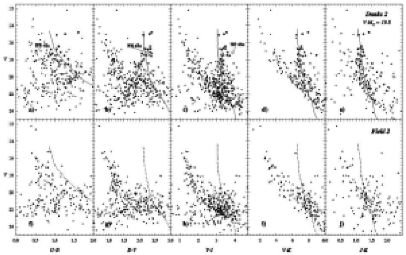
Figure 5: Optical CMDs of stars located in $D2$ and $F2$ zones. See also Sect 3.1 and Fig 1 for zone definitions. Symbols and curves are the same as in Fig 3

3.1 Selection of zones

With the aim of simplifying the analysis of the data, the studied region was divided into several sets presented in Table LABEL:tab:zones (see also Fig. 1):

Table 3: Description of studied zones.

$Name$	$Shape$	$Center$	$Radius~{}(r)$
$D1$	circle	Danks 1	$r=0\aas@@fstack{\prime}96$
$F1$	corona	Danks 1	$0\aas@@fstack{\prime}96<r<1\aas@@fstack{\prime}36$
$D2$	circle	Danks 2	$r=1\aas@@fstack{\prime}44$
$F2$	corona	Danks 2	$1\aas@@fstack{\prime}44<r<2\aas@@fstack{\prime}04$
$DBS130$	circle	DBS2003 130	$r=0\aas@@fstack{\prime}72$
$F130$	corona	DBS2003 130	$0\aas@@fstack{\prime}72<r<1\aas@@fstack{\prime}02$
$DBS131$	circle	DBS2003 131	$r=0\aas@@fstack{\prime}72$
$F131$	corona	DBS2003 131	$0\aas@@fstack{\prime}72<r<1\aas@@fstack{\prime}02$
$Field$	The remaining observed area

In this manner, $D1$, $D2$, $DBS130$ and $DBS131$ correspond to the regions involving the studied clusters and their surrounding areas; while $F1$, $F2$, $F130$ and $F131$ correspond to the respective, adopted, comparison field for each cluster. We emphasize two facts: a) each comparison field covers the same sky area as the corresponding cluster region, and b) as will be explained in Sec. 3.3.2, embedded cluster BDS2003 132 was not included in the present study.

3.2 Photometric diagrams

The Two Color Diagrams (TCDs) and Color Magnitude Diagrams (CMDs) of the different zones are shown in Figs. 2- 10 in a self explanatory format (see also Sect. 3.1).

The TCDs of the cluster zones (Figs. 2, 4 and 7) show clearly the presence of the, expected, field population along with a heavily reddened ($E_{B-V}\sim 2.5$) group of stars, most likely cluster members. In all studied zones $B-V$ vs. $V-I$ diagrams confirm the above mentioned trend and show that the clusters members suffer abnormal reddening laws, unlike the field population which follow a normal one. As a consequencem individual $R$ ($=A_{V}/E_{B-V}$) values were derived for each cluster.

The optical CMDs of the cluster zones (Figs. 3, 5 and 8) also illustrate that the cluster populations is made of very reddened stars. According to the infrared CMDs, 2MASS data have not enough precision to improve the information obtained from the optical photometric diagrams. However, it is important to notice that the chosen distance for each cluster (see Sect. 3.3) produced a coherent fit of the ZAMS or MS along all the CMDs (optical and infrared) as lower envelopes of the adopted member stars.

3.3 Main objects in the studied region

Table 4: Parameters of the analyzed stellar groups

Stellar group	Center		$E_{B-V}$	$R$	$V-M_{V}$	$A_{V}$	$V_{0}-M_{V}$	Age[Myr])	IMF slope
	$\alpha_{2000}$	$\delta_{2000}$
Danks 1	13:12:27.0	-62:41:59.7	2.45	4.0	19.80	9.8	10.0	$\sim$ 5	$\sim$ 1.5
Danks 2	13:12:55.3	-62:40:42.0	2.40	3.6	19.83	8.7	11.5	$\sim$ 5	$\sim$ 1.1
DBS2003 130	13:11:54.0	-62:47:02.0	2.3	$\sim$4.5	$\sim$24.9	10.4	14.5	$\sim$ 1-3	-
DBS2003 131	13:11:39.4	-62:33:11.5	2.6	$\sim$4.5	$\sim$25.2	11.7	13.5	$\sim$ 1-3	$\sim$ 0.98 - 1.5
Foreground	13:12:43.4	-62:39:02.2	$\sim$0.5	3.1	$\sim$9-11	$\sim$1.5	$\sim$7.5-9.5	-	-
Note 1: Foreground coordinates correspond to the center of the observed area (see Fig. 1)
Note 2: IMF slope values for DBS2003 131 were taken from Leistra et al. (2005) and included for comparison.

3.3.1 Danks 1 and Danks 2

Danks 1 (C1309-624) and Danks 2 (C1310-624) are catalogued as open clusters with a diameter of $1\aas@@fstack{\prime}0$ and $1\aas@@fstack{\prime}5$, respectively, and both classified with a Trumpler class 1-1-p- (Lyngå 1987; Dias et al. 2002). That is why the sizes of the respective regions ($D1$, $F1$, $D2$ and $F2$) were chosen (see Sect. 3.1) to analyze the cluster itself and the behavior of its associated field respectively. Although these clusters are more easily detectable in infrared still they appear as clear over-densities in DSS-2 (Fig. 1a). The adopted centers for the clusters were taken from $SIMBAD$ and are presented in Table LABEL:tab:param. Photometric diagrams of these clusters (Figs. 2 - 5) show (i) they suffer substantial reddening ($E_{B-V}=2.45$ for Danks 1 and 2.4 for Danks 2); (ii) exhibit abnormal $R$ value (3.6 - 4.0); and (iii) may also suffer a differential reddening across selected regions. In order to perform membership assignment, the individual position of the stars in all the photometric diagrams have been carefully inspected aiming at checking their consistency in all these diagrams simultaneously. This later point was performed assuming we were dealing with young populations and the stars positions on the CMDs were close to the location of a compatible ZAMS solution, by using previously adopted color excess ratios and color excess values. However, we allow for some dispersion around the adopted ZAMS due to the probable presence of dust inside the cluster, and also due to photometric errors (mainly in $U$ band). As a following step, we took into account the number of stars for each magnitude bin according to the apparent LFs (see Baume et al. 2004ab, 2006). This procedure was applied for all stars down to an adopted $V_{lim}\sim 19$. At fainter magnitudes, contamination by field stars becomes severe, preventing an easy identification of faint cluster members. The fit of a properly reddened Schmidt-Kaler (1982) ZAMS to the blue edge of the adopted member stars yields a distance modulus $V_{0}-M_{V}=10.0\pm 0.3$ for Danks 1 and $V_{0}-M_{V}=11.5\pm 0.3$ for Danks 2 (errors from eye inspection). An age of about 5 Myr can be estimated for both clusters taking into account Meynet et al. (1993) calibration. It must be noticed that distance values are lower than those obtained in previous works (e.g. Bica et al. 2004) and this is mainly due to the abnormal extinction law that we derive and adopt in the present study.

To compute the clusters LFs and IMFs the following procedure was adopted:

• Stars located in cluster zones ($D1$ and $D2$) and comparison zones ($F1$ and $F2$) were selected. Additionally, in order minimize the contamination of stars from the field population, only those stars with $V-I>(V-I)_{lim}$ were considered (values of $(V-I)_{lim}$ equal to 3.4 and 3.0 were adopted for $D1/F1$ and $D2/F2$ respectively). All these stars were called then ”red stars”

• The apparent LFs of the clusters were obtained substracting the apparent LF of ”red stars” in the corresponding comparison zone ($F1$ or $F2$) from the apparent LF of ”red stars” placed in the clusters zones ($D1$ or $D2$). Bins were chosen in a way to avoid negative final values.

• The resulting apparent LFs were shifted in magnitude to correct them by absorption and distance and to obtain the final LFs.

• Finally, the IMFs of the clusters were computed converting LFs bins into mass bins using the mass-luminosity relation given by Scalo (1986).

The resulting apparent LFs and IMFs are presented in Table LABEL:tab:alf and Fig. 6 respectively, together with the corresponding IMFs slopes.

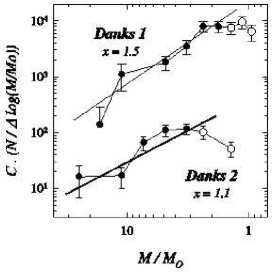
Figure 6: Initial Mass Functions (IMFs) of Danks 1 (upper plot) and Danks 2 (lower plot). Error bars are from Poisson statistics. The least square fittings for the more massive bins are indicated by solid right lines (open circles indicate bins not used in the fits. See text for details). For clarity, each IMF was shifted by an arbitrary constant (“$C$”).

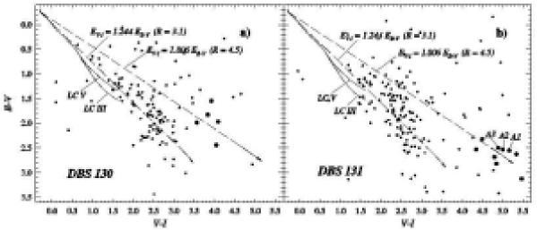
Figure 7: Optical TCDs of stars located in $DBS130$ and $DBS131$ zones. See also Sect. 3.1 and Fig 1 for zone definitions. Symbols and curves are the same as in Fig. 2

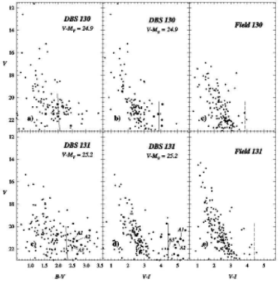
Figure 8: Optical CMDs of stars located in $DBS130$, $F130$, $DBS131$ and $F131$ zones. See also Sect. 3.1 and Fig 1 for zone definitions. Symbols and curves are the same as in Fig 3. $A1$, $A2$ and $A3$ are stars identification from Leistra et al. (2005).

Table 5: Apparent Luminosity Functions.

Danks 1		Danks 2
$\Delta V$	N	$\Delta V$	N
14.0-16.0	1	14.0-16.0	3
16.0-18.0	4	16.0-17.0	6
18.0-19.0	13	17.0-18.0	12
19.0-20.0	12	18.0-19.0	20
20.0-21.0	22	19.0-20.0	20
21.0-22.0	20	20.0-22.0	14
22.0-23.0	16	22.0-24.0	12
23.0-24.0	17	24.0-26.0	0
24.0-25.0	10

3.3.2 Embedded clusters

The region under study contains three recently detected (Dutra et al. 2003) embedded clusters. They were identified as BDS2003 130, 131 and 132. Each cluster is respectively found very near to the HII regions G305.27-0.01, G305.3+0.2 and G305.3+0.1, which can also be identified respectively with the S155, S156 and S154 bubbles from the Churchwell et al. (2006) catalogue.

Our observations allowed us to obtain reliable information for BDS2003 130 and 131. Unfortunately BDS2003 132 is too near to the position of star HD 114515 preventing to reach faint magnitudes. Both BDS2003 130 and BDS2003 131 (= G305.3+0.2) are not visible in Fig. 1a, and their presence is suggested only in our deep frames (see Fig. 1b and d). Nevertheless, the CMDs of their zones ($DBS130$ and $DBS131$) clearly trace their presence, especially when the diagrams are compared with their respective comparison fields ($F130$ and $F131$) as shown in Fig 8. Additionally, their TCDs (Fig. 7) reveals that both cluster suffers an abnormal extinction law and a $R\sim 4.5$ value is adopted for them. It must be noticed that since almost all the considered cluster stars are at the limit of our photometry, their individual values must be taken as preliminary estimations and only the group structure in the diagrams can be considered valid. Still, stars indicated with black circles in the photometric diagrams can be considered as very probable YSOs. In this way, it is possible to obtain an estimation of their parameters considering they are suffering a similar reddening than Danks 1/2 ($E_{B-V}\sim 2.5$). This assumption is coherent with the $B-V$ values ($\sim 2.1-2.4$) of assumed YSOs members. To estimate their distances, we again use a shifted Schmidt-Kaler (1982) ZAMS. The obtained clusters parameters are presented in Table LABEL:tab:param. In the case of BDS2003 131, the distance is comparable with that derived in other studies (Leistra et al. 2005; Longmore et al. 2007) based on near infrared data or kinematic modeling of the related HII region (see Churchwell et al. 2006).

Table 6: Photometric data and adopted parameters for WR 48a.

Photomety		Parameters
$U$	19.89	$E_{B-V}$$~{}\sim~{}$	2.4
$B$	19.37	$R_{ISM}$$~{}\sim~{}$	3.8
$V$	17.13	$(A_{V})_{ISM}$$~{}\sim~{}$	9.1
$I$	13.25	$(A_{V})_{CSM}$$~{}\sim~{}$	2
$J$	8.74	$V_{O}-M_{V}$$~{}\sim~{}$	10.9
$H$	6.80	$M_{V}$$~{}\sim~{}$	-4.9
$K$	5.09

Note 1: $JHK$ photometry was taken from 2MASS catalogue

Note 2: $M_{V}$ was taken from Lundström & Stenholm (1984)

3.3.3 Star WR 48a

WR 48a is a WC9 star (Danks et al. 1983) and it is placed within $\sim 1^{\prime}$ of the clusters Danks 1/2. The distance estimation performed by Danks et al. (1983) was of 4 kpc, however van der Hucht (2001) concluded it was only about 1.2 kpc away. On the other hand, Danks et al. (1983) estimation of the absorption that this star is suffering is $A_{V}\sim 9.2$. This value is compatible with the values found for Danks 1/2 (see Table LABEL:tab:param). Notwithstanding WR stars can involve circumstellar envelopes producing intrinsic absorption, seems reasonable to associate WR 48a star to the clusters Danks 1/2 distance. Given the photometric values obtained for this star (see Table LABEL:tab:wr) and its position in the CMDs of the clusters it results compatible with being probable run away member as was previously assumed by Lundstrom & Stenholm (1984) In this case the average values of the parameters between Danks 1/2 can be assumed for the WR star. In this way, the absorption value comes only from the interstellar medium ($(A_{V})_{ISM}$) and adopting also $M_{V}=-4.9$ value from Lundström & Stenholm (1984) for a WC9 star, it is possible to estimate the circumstellar absorption ($(A_{V})_{CSM}$). All the obtained values are presented in Table LABEL:tab:wr and they indicate that only a minor amount of the total visual absorption is produced by the stellar envelope.

3.4 The Field

The comparison of the photometric diagrams (TCDs and CMDs) of the field region are presented in Figs. 9 - 10. The $U-B$ vs. $B-V$ diagram reveals the presence of a relatively small group of blue stars (black symbols). On the other hand, all the CMDs show two clear parallel blue and red sequences.

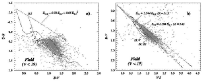
Figure 9: Optical TCDs of stars located in $Field$ zone. See also Sect 3.1 and Fig 1 for zone definitions. Curves are the same as in Fig 2.

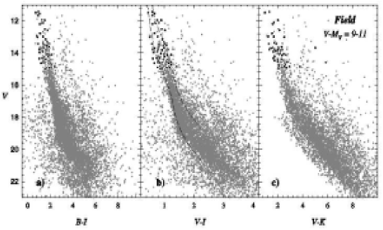
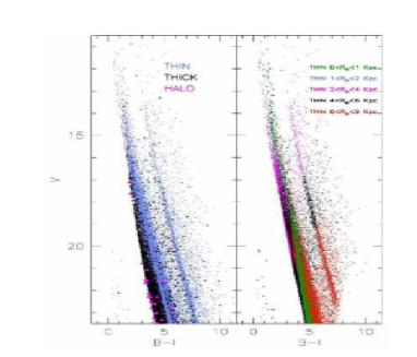
Figure 10: Left plots: Observational optical CMDs of stars located in $Field$ zone, see Sect. 3.1 and Fig 1 for zone definitions. Curves are the same as in Fig. 3. Right plots: A simulation of the CMDs corresponding to the Galactic contribution along the ($l,b$)$=$($305,37^{\circ}+0.12^{\circ}$) line of sight. The left panel highlights the different contribution of the thin/thick disk and halo populations and the right panel shows the same simulation but analyzing the distribution of the thin disk population at different distances along the line of sight. The red oblique sequence is best explained as due to the projection of giants and red clump stars at different distances.

For a deeper understanding of these diagrams, and in particular that of the parallel red sequence, we make a comparison between the observed diagrams and that of the expected Galactic contribution along this line of sight. The later is estimated by making use of the Robin et al. (2003) Galactic model which provides synthetic CMDs at any given Galactic coordinates. These synthetic diagrams have been successfully used (e.g. Momany et al. 2004, 2006) to explain the presence of other seemingly anomalous features around Galactic open clusters. Figure 10 (see the colored version) compares the observed $V$ vs. $B-I$ CMD with the expected Galactic contribution along the ($l$,$b$) = ($305.37^{\circ}$,$+0.12^{\circ}$) line of sight according to the Besançon simulation . In the middle panel of the right plot (of Fig. 10) we first disentangle between the stellar populations belonging to the three simulated Galactic main components (thin and thick disks plus halo) in this direction. Clearly, the simulation shows that we expect little, if any, halo contribution, and that most of the Galactic contribution is due to thin disk populations. The true nature of the red and oblique sequence is best explained in the right panel of the plot. Indeed, when analyzing the distance distribution of the thin disk populations, the location of the red oblique sequence is re-constructed as the projection of red clump stars and bright giants at different distances.

Additionally, the use of the Schmidt-Kaler ZAMS (1982) indicates that the brighter part of the blue sequence (black symbols in left panel of Fig 10) is associated with a nearby group of stars with $E_{B-V}\sim 0.5$ and a distance modulus $V-M_{V}\sim 9-11$, corresponding to about 350-750 pc.

4 Discussion

4.1 The Galactic spiral structure in Carina and Centaurus regions

Previous investigations by our group (Vázquez et al. 2005; Carraro & Costa 2009) presented optical observations near the field addressed in this paper. The multiple young and blue populations along the line of view was found to reveal reveal three different spiral features at increasing distance from the Sun..

In this paper, we strengthen this conclusion and lend further support to the presence of at least three populations in this Galactic sector: (i) the first is a spatially spread foreground population placed mainly between 350-750 pc; (ii) the second is situated just behind a very dark cloud at 1-3 kpc and is represented by the clusters Danks 1/2; (iii) and, finally, a third population which is traced by the embedded clusters, located at about 5-7 kpc.

The results are illustrated in Fig. 11 where the Vallée (2005) spiral arms’ model is also shown as dotted curves. In this plot we summarized the recent findings of Carraro & Costa (2009), Vázquez et al. (2005) and the present study. The various the segments indicate the location and corresponding uncertainties of the different populations detected along the $l=290^{\circ}$, $305^{\circ}$ and $306^{\circ}$ line of sight.

We confirmed the early findings by Vázquez et al. (2005) that the populations beyond the open cluster Stock 16 (their groups A and B) are most probably associated to Scutum-Crux. The same association could tentatively be done for the embedded clusters studied in this paper. The Danks 1/2 clusters, on the other hand, clearly belong to the Carina branch of the Carina-Sagittarius arm, like Stock 16 and the population A described in Carraro & Costa (2009). In this scenario it appears however that the Scutum-Crux arm as traced by Vallée should have a larger pitch angle than 11^∘. In fact his plots indicate this parameter has a $\sigma\approx 4^{\circ}$. However, some alternative scenarios are viable: (i) the observed displacement from the model can be accounted for by the natural width of 1 Kpc for spiral arms (see Vallée 2005), or (ii) the two most distant groups falling in between Scutum-Crux and Carina are tracing an inter-arm structure, or a branch of Carina. This later possibility finds some support from the existence of several HII regions at the same position of these two groups (Russeil 2003; Paladini 2004; see also Fig. 11).

More directions close in this regions have to be studied. For example, more deeper, detailed and complementary analysis in different wavelengths as optical and infrared by using objects as embedded clusters seems necessary to better trace the spiral structure in the fourth Galactic quadrant.

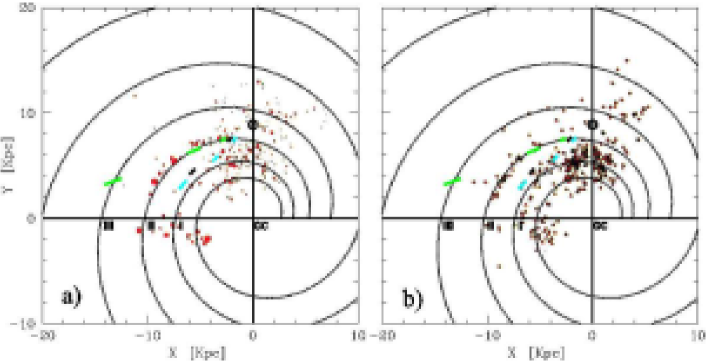
Figure 11: The groups we discuss in this paper are here superposed to the Vallée (2005) model of Galactic spiral structure (dotted curves) together with some of the HII regions (red symbols) adapted from Russeil (2003) in left panel (a) and Paladini et al. (2004) in right panel (b). Our groups are indicated as solid black segments representing their location and distance error. The green groups have been discussed in Carraro & Costa (2009) and are located at $l=290^{\circ}$, whilst the blue groups have been studied by Vázquez et al. (2005) toward $l=306^{\circ}$. The symbols I, II and III indicate the Scutum-Crux, Carina-Sagittarius and Perseus arms, respectively. See text for more details.

4.2 Cluster IMFs

There is an important spread in the IMFs slopes computed for massive stars among several young cluster in the Galaxy. This is not yet fully understood, and can be attributed to the fact that (a) the IMF may not have a universal shape or/and (b) there are intrinsic mistakes in its computation (Scalo 1998).

Considering then the IMF slope given by:

$x=-log(dN/dlogM)/logM$,

where $dN$ is the number of stars within the logaritmic mass interval $dlogM$ around $logM$. The widely accepted slope values are $x=1.35$ (Salpeter 1955) or $x=1.7$ (Scalo 1998). However, in several very young open clusters (age $<10^{7}$ yr, see e.g. Baume et al. 1999, 2003, 2004ab and references therein) we detect lower values for this parameter.

Our computed values for the clusters Danks 1/2 together with the value obtained by Leistra et al. (2005) for DBS2003 131 are presented in Table LABEL:tab:param. The results are coherent and lie within the range of typically accepted values for very young clusters. However, we remark that our derived IMFs and their slopes values are influenced by poor statistics.

5 Conclusions

A uniform and deep study was performed in a region of the Galactic plane towards $l=305^{\circ}$. This region includes the open clusters Danks 1/2, their surrounding field and also three embedded IR clusters. The main properties of the different populations located along this line of sight were derived and a description of interstellar medium (through the color excess behavior) has allowed us to sketch a better picture of the observed clusters in this Galactic direction. In particular, the basic parameters of Danks 1/2, DBS2003 130 and DBS2003 131 were determined. It must be noticed that the method used analyzing star by star and the inclusion of near ultraviolet $U$ data has helped us obtain mean distance values for the open clusters that are quite different from those derived in recent papers, where the latter are based on the analysis of only the global morphology of the CMDs. Additionally, our optical methods applied for classical embedded clusters offer compatible results with those especific ones used in infrared, giving then more reliability to the results achieved in both cases. Our results indicate that, in order to obtain better picture of complex and reddened regions, near ultraviolet data are necessary. The performed analysis indicates that Danks 1/2 are almost at the same distance from the Sun, located probably on the Scutum-Crux arm. The analysis of the location of these grouping, together with previous detections in the same portion of the disk, are helping us to get a better picture of the spiral structure of the inner Milky Way.

Additionally, rough estimates of the IMFs for both objects were computed for the first time. The derived slope values were similar to those of other studied addressing young open clusters. Lastly, the optical photometric values of WR 48a were presented and its main parameters were estimated, considering it as a runaway member of Danks 1/2.

References

- [1] Baume G., Moitinho A., Giorgi E.E., Carraro G. & Vázquez R.A. 2004a, A&A 417, 961
- [2] Baume G., Vázquez R.A. & Carraro G. 2004b, MNRAS 355, 475
- [3] Baume G., Moitinho A., Vázquez R.A., Solivella G., Carraro G., Vilanova, S. 2006, MNRAS 367, 1441
- [4] Bica E., Ortolani S., Momany Y., Dutra C.M. % Barbuy B. 2004, MNRAS 352, 226
- [5] Carraro G. & Costa E. 2009, A&A 493, 71
- [6] Churchwell E., Povich M.S., Allen D., Taylor M.G., Meade M.R., Babler B.L., Indebetouw R., Watson C. et al. 2006, ApJ 649, 759
- [7] Clark J.S. & Porter J.M. 2004, A&A 427, 839
- [8] Cousins A.W.J. 1978a, MNSSA 37, 62
- [9] Cousins A.W.J. 1978b, MNSSA 37, 77
- [10] Cutri R.M., Skrutskie M.F., Van Dyk S. et al. 2003, University of Massachusetts and Infrared Processing and Analysis Center (California Institute of Technology)
- [11] Danks A.C., Dennefeld M., Wamsteker W. & Shaver P.A. 1983, A&A 118, 301
- [12] Dias W.S., Alessi B.S., Moitinho A., et. al 2002, A&A 389, 871
- [13] Dutra C.M., Bica E., Soares J. & Barbuy B. 2003, A&A 400, 533
- [14] Girardi L., Bressan A., Bertelli G., & Chiosi C. 2000, A&AS 141 371
- [15] Koornneef J. 1983, A&A 128, 84
- [16] Landolt A.U., 1992, AJ 104, 340
- [17] Leistra A., Cotera A.S., Liebert J. & Burton M. 2005, AJ 130, 1719
- [18] Longmore S.N., Maercker M., Ramstedt S. & Burton M.G. 2007, MNRAS 380, 1497
- [19] Lundström & Stenholm 1984, A&AS 58, 163
- [20] Lyngå G. 1987, Catalog of Open Star Cluster Data, Strasbourg, CDS
- [21] Meynet G., Mermilliod J.-C. & Maeder A. 1993, A&AS 98, 477
- [22] Momany Y., Zaggia S., Gilmore G., Piotto G., Carraro G., Bedin L R. & de Angeli F. 2006, A&A 451, 515
- [23] Momany Y., Zaggia S. R., Bonifacio P., Piotto G., De Angeli F., Bedin L. R. & Carraro G. 2004, A&A 421, L29
- [24] Paladini R., Davies R.D. & DeZotti G. 2004, MNRAS 347, 237
- [25] Robin A. C., Reylé C., Derrière S. & Picaud S. 2003, A&A 409, 523
- [26] Russeil D. 2003, A&A 397, 133
- [27] Salpeter E.E. 1955, ApJ 121, 161
- [28] Scalo J. 1986, Fund. Cos. Phys. 11, 1
- [29] Scalo J. 1998, in The Stellar Initial Mass Function, 38th Herstmonceux Conference, ASP Conf. Ser., 142, 201
- [30] Schmidt-Kaler Th. 1982, Landolt-Börnstein, Numerical data and Functional Relationships in Science and Technology, New Series, Group VI, Vol. 2(b), K. Schaifers and H.H. Voigt Eds., Springer Verlag, Berlin, p.14
- [31] Skrutskie M.F., Cutri R.M., Stiening R. et al. 2006, AJ 131, 1163
- [32] Stetson P.B. 1987, PASP 99, 191
- [33] Stetson, P.B. 1992, in Stellar Photometry-Current Techniques and Future Developments, ed. C. J. Bulter, & I. Elliot (Cambridge: Cambridge University Press), IAU Coll., 136, 291
- [34] van der Hucht K.A. 2001, NewAR 45, 135
- [35] Vallée J.P. 2005, AJ 130, 569
- [36] Vázquez R.A., Baume G., Feinstein C., Nuñez J.A. & Vergne M.M. 2005, A&A 435, 883