Evidence for a geomagnetic effect in the CODALEMA radio data

Abstract

The CODALEMA experiment detects the cosmic air showers with an hybrid detector composed of an array of scintillators and an array of antennas triggered by the particle array. We will first describe the experiment and the data analysis then we will focus on the sky distribution of the events detected by the antennas which presents a strong asymmetry. We will show that this asymmetry is well described and quantified at first order by an emission of the shower electric field given by the cross product of the shower axis with the geomagnetic field vector. The physical origin of this term is explained in another talk in this conference.

radiodetection, geomagnetic, CODALEMA

1 Introduction

The radiodetection of cosmic air showers is studied by three experiments: two in Europe (CODALEMA, France [1] and LOPES, Germany [2]) and one in Argentina, at the heart of the Pierre Auger Observatory (see [3, 4]). The main goal of the CODALEMA experiment, located at the Nançay radio observatory, is the study of the electric field generated by the charged particles of air showers created by the interaction of primary cosmic rays in the atmosphere, at energies between $10^{16}$ and $10^{18}$ eV. We are currently using two different instruments: a particle array of 17 scintillators and a radio array of 24 antennas. The radio array is triggered by the particle array. The estimation of the shower axis, core position and primary energy is provided by the particle array and used as a reference by the radio array. The detector setup is presented in Fig. 1.

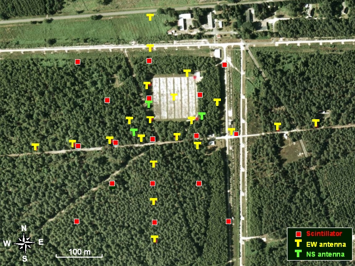
Figure 1: Schematic view of the CODALEMA experiment. The particle array is represented by the squares. The radio array is indicated by the letters “T”.

The scintillators cover an area of $340\times 340$ m² and the distance between them is $85$ m. The antennas form a cross with two arms of $600$ m length. The 14 antennas on the North-South (NS) and East-West (EW) arms are used in this study and these antennas measure the EW polarization of the incoming electric field. We will also discuss in section 6 the preliminary results we got with the 3 antennas measuring the NS polarization.

2 The particle array

Each particle detector is a plastic scintillator observed by two photomultipliers with different high voltage gains in order to ensure a dynamic range between $0.3$ and $3\,000$ Vertical Equivalent Muons (VEM). The detectors are wired to a central shelter containing the power supplies and the complete acquisition. The start time and integrated signal of the ADC trace is computed for each scintillator. The shower axis position, the core position and the estimation of the number of particles reaching ground are computed using a curved shower front and a Nishimura-Kamata-Greisen function. Finally, the conversion of ground particle densities to primary energy is obtained with the Constant Intensity Cut (CIC) technique which defines a vertical equivalent shower size $N_{0}=N(\theta=0^{\circ},E)$. AIRES [5] simulations give the formula $E_{0}=2.14\times 10^{10}~{}N_{0}^{0.9}$ with a resolution of $\Delta E/E\sim 30\%$ at $10^{17}$ eV assuming protons as primaries. This resolution is mainly due to shower-to-shower fluctuations and to the nature of the primary. The reconstructed events are classified according to their core position: internal events are those where the particle density is larger for internal detectors than for external detectors lying on the sides of the array. In this case, the core is contained inside the array and we have a satisfactory accuracy for both shower core and size. Energy estimation is meaningful only for internal events; external ones have less reliable shower parameters for core position and size but the axis position can be used for further analysis.

The trigger condition requires the 5 central scintillators to have a signal above $0.3$ VEM within a time window of $600$ ns. The average event rate is around 8 events each hour.

3 The radio array

A single radio detector is constituted by a fat active dipolar antenna made of two $60$ cm long, $10$ cm wide aluminium slats of $1$ mm thickness separated by a $1$ cm gap and hold horizontally above the ground by a $1$ m plastic mast. The signal is preamplified by a dedicated, high input impedance, low noise (1 nV.Hz^-1/2), $36$ dB amplifier with a $100$ kHz-$220$ MHz bandwidth at $3$ dB. To avoid intermodulation due to a $2$ GW local emitter, the signal is high-pass filtered ($20$ dB at 162 kHz). The 14 antennas are triggered by the particle array; the digitization is done by a fast 12 bits ADC running at $1$ GHz with a memory depth of $2\,560$ points (corresponding to $2.5~{}\mu$s).

The offline analysis first filters the signal in the $23-83$ MHz band after correction for the cable frequency response. We use the galactic radio background to adjust the relative gains. In this frequency band, the pulse corresponding to the transient event is found using the Linear Prediction Method [6]. Then, the pulse is associated to an absolute time and a signal value. From the time information of the tagged antennas we can reconstruct an arrival direction by simple triangulation. Using the time information of the two arrays, we have two independent measurements of the shower axis and impact time which can be compared in order to identify unambiguously cosmic shower seen by the radio array. The set of events seen by the radio array is consituted of events having an angular difference smaller than $20^{\circ}$ and a time difference in the interval $[-100,100]$ ns, as illustrated in Fig. 2.

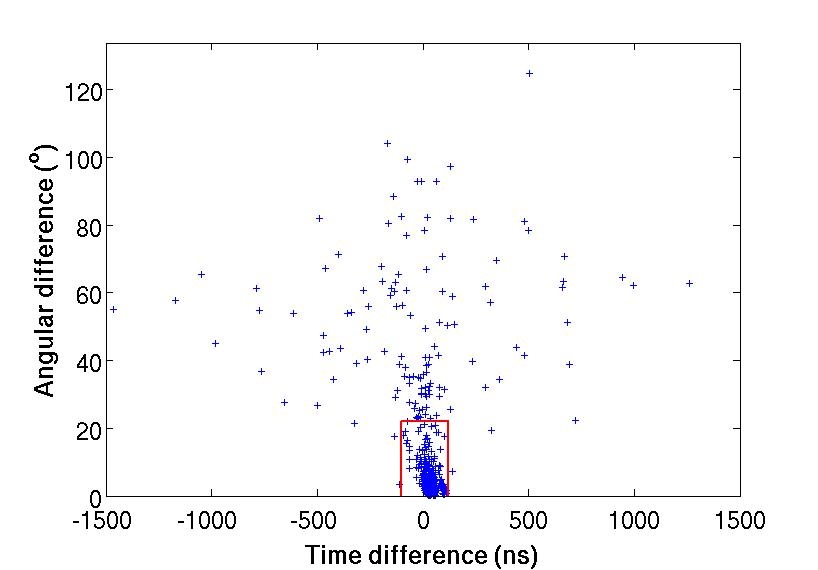
Figure 2: Selection of the actual cosmic events detected by the radio array using the angular difference and the time difference between the two independent reconstructions; the box indicates the criteria for coincidences: angular difference smaller than $20^{\circ}$ and time difference in the interval $[-100,100]$ ns.

4 Radio detection efficiency

The data set presented in this analysis has been recorded between November $27^{\mathrm{th}}~{}2006$ and March $20^{\mathrm{th}}~{}2008$ corresponding to $355$ effective days of stable data acquisition. The numbers of internal events in this period are summarized in Table 1.

Table 1: Number of events.

events	scintillators	antennas	coincidences
reconstructed	$61\,517$	$750$	$619$
internal	$28\,128$	$195$	$157$
$E>10^{16}$ eV	$7\,889$	$169$	$154$
$E>5\times 10^{16}$ eV	$692$	$134$	$129$

The energy threshold of the radio array appears to be around $10^{17}$ eV and that of the particle array around $10^{15}$ eV. The efficiency of the radio array is defined as the ratio of the number of radio events to the number of particle events in a given energy range. This efficiency is presented in Fig. 3. It is increasing regularly above $3\times 10^{16}$ eV and reaches $50\%$ at $2\times 10^{17}$ eV. Taking into account the properties of the electric field generated by the geomagnetic field permits to be compatible with a full efficiency at high energy, as argued in section 6.

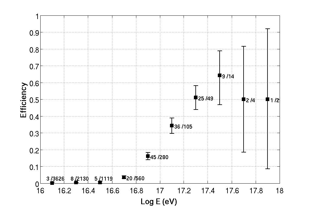
Figure 3: Efficiency of the radio array defined as the ratio of the number of radio events to the number particle events in a given energy bin.

5 Asymmetry in the radio events

We first focus on the list of all events seen in coincidence between the particle array and the radio array, including external events for which the axis position only is known. The projection on a sky map of the arrival directions of these events is presented in Fig. 4.

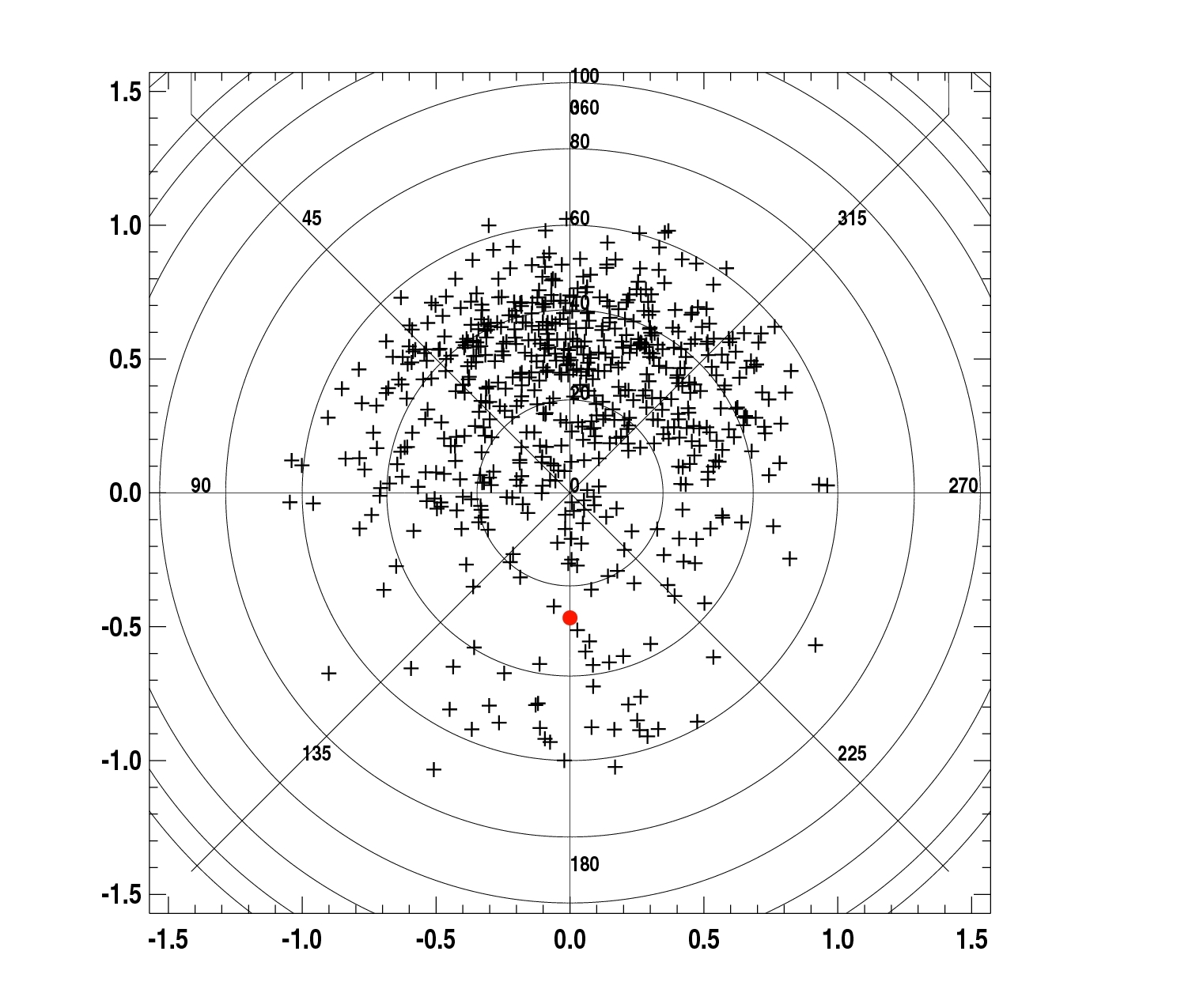
Figure 4: Sky map of observed radio events. The zenith is at the center and the azimuths are: North (top, $0^{\circ}$), West (left, $90^{\circ}$), South (bottom, $180^{\circ}$), East (right, $270^{\circ}$). The geomagnetic field is indicated by the dot.

We clearly observe a strong relative excess of events coming from the North. The ratio of the number of events coming from the South (ie with azimuth $90^{\circ}<\phi<270^{\circ}$) to the total number of events is $n_{\mathrm{South}}/n_{\mathrm{tot}}=109/619=0.17\pm 0.02$. This asymmetry is not expected a priori because:

• the geometrical setup of the CODALEMA experiment is symmetric and presents no instrumental bias;

• the azimuthal distribution of the particle array (remind that it also provides the trigger of the radio array) is compatible with a flat distribution.

We compared the observed sky map to the sky map one could naively have expected, namely a symmetrized version of the coverage map obtained from the particle zenithal distribution with a flat azimuthal distribution: the discrepancy reaches 16 standard deviations. We verified that the asymmetry level is independent of the data set: 7 independent time ordered sets of events give similar values of the ratio $n_{\mathrm{South}}/n_{\mathrm{tot}}$ (around $0.17$).

If we restrict the data set to internal events (with an estimation of the primary energy), we observe that when the energy increases, the asymmetry level becomes compatible with the symmetric value of $n_{\mathrm{South}}/n_{\mathrm{tot}}=0.5$, as shown in Fig. 5. The ratio $n_{\mathrm{East}}/n_{\mathrm{tot}}$ is always compatible with $0.5$.

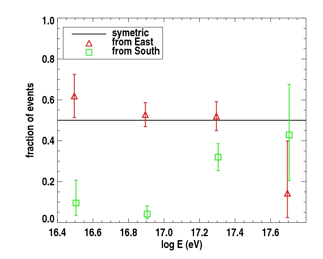
Figure 5: Evolution of the ratio $n_{\mathrm{South}}/n_{\mathrm{tot}}$ as a function of energy (energy bins are independent). A ratio of 0.5 indicates symmetry. At high energy, the observed radio sky map become compatible with a symmetric map in both NS/EW sectors.

We can therefore conclude that the asymmetry observed by the radio array is due to an energy threshold effect.

6 Semi-empirical model

The detected asymmetry is clear and unambiguous. In order to understand its origin, we can think about the effect of the geomagnetic field on the charged secondary particles of the shower. The associated Lorentz force acting on these particles is responsible for the emission of the electric field. We can therefore expect a rough dependence of the global macroscopic electric field on a Lorentz term such as $\vec{E}\propto\vec{v}\times\vec{B}$ where $\vec{v}$ is the shower axis direction and $\vec{B}$ the geomagnetic field. The EW-oriented dipolar antennas will be sentitive to the EW component of this electric field $(\vec{v}\times\vec{B})_{\mathrm{EW}}$. To build the expected event map, we must also take into account the zenithal distribution of the particle array which triggers the radio array. We used for this the following parametrization:

$$\frac{\mathrm{d}N}{\mathrm{d}\theta}=(a+b\,\theta)\frac{\cos\theta\sin\theta}{1+\exp((\theta-\theta_{0})/\theta_{1})},$$

with $a=44.96$, $b=0.57$, $\theta_{0}=49.18^{\circ}$, $\theta_{1}=5.14^{\circ}$, computed using the internal events above $10^{17}$ eV. The resulting expected events density sky map taking into account all these ingredients is presented in Fig. 6, assuming that the number of events is proportionnal to the amplitude of the electric field.

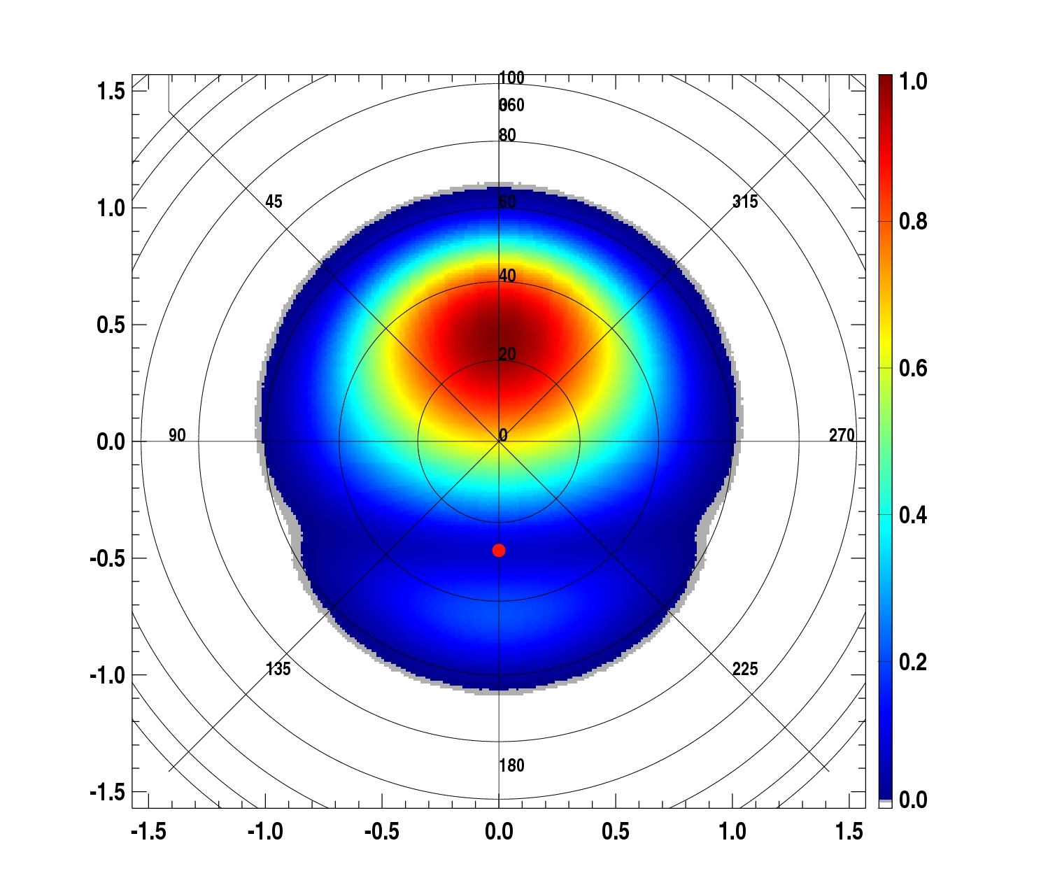
Figure 6: Expected EW density map according to the semi-empirical model. See text for details.

An efficient way to test the validity of this semi-empirical model is to compute an ensemble average of the angular distributions of a large number of realisations of $N$ simulated events following the expected density map, where $N$ is the actual number of detected events in a given polarization: $N=619$ for the EW polarization and $N=100$ for the NS polarization.

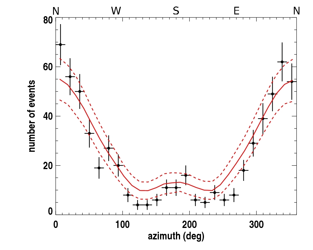
(a) Azimuthal distribution for the EW polarization.

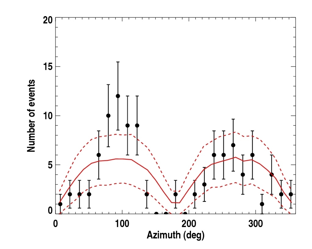
(b) Azimuthal distribution for the NS polarization.

Figure 7: Comparison of the expected azimuthal distributions to the observed azimuthal distributions (crosses) in the EW polarization (Fig. (a) and (b)) and in the NS polarization (Fig. (c) and (d)). The lines correspond to the simulated azimuthal distributions obtained after $1\,000$ realisations of $619$ events and $100$ events for the EW and NS polarizations respectively with the associated $\pm 1\sigma$ error bands.

In our case, for the EW and NS polarization, the zenithal observed and simulated distributions are in very good agreement; Figures 7a and 7b present the results for the azimuthal distributions. The semi-empirical model reproduces correctly the main features of the observed azimuthal distributions: for the EW polarization we have a maximum towards the North, a local maximum towards the South and minima in the East and West directions; for the NS polarization we have events in both East and West hemisphere and no events coming from the North and the South, in agreement with the semi-analytical model. The semi-analytical model describes remarkably well the angular distributions in both EW and NS polarizations. The study of the polarity of the electric field can be found in [7] and in another contribution to this conference [8].

The model permits to understand the shape of the sky distribution but can also be used to check the radio detection efficiency as a function of the geometrical factor $\vec{v}\times\vec{B}$. For the EW polarization (for which we have higher statistics), when plotting the ratio of the number of radio detected events to the total number of events as a function of $(\vec{v}\times\vec{B})_{\mathrm{EW}}/|vB|$, we find a linear increase from $0$ to $1$ which validates our assumption that the number of detected events is directly linked (nearly proportional) to the electric field value. We observe that in order to be detected, events with a low value of the Lorentz force EW component (as it is the case for events coming for instance from East or West) must have a higher energy than events with high values, coming from North. At the highest energies, all events are detectable independently of their arrival direction and the radio efficiency will become independent of the Lorentz force component. In Fig. 3, the radio efficiency was plotted as a function of the energy given by the particle array. If we rescale this energy according to the semi-analytical model $E^{\prime}=E\,.\,(\vec{v}\times\vec{B})_{\mathrm{EW}}/|vB|$, we obtain an efficiency which saturates at $100\%$ above the threshold energy $E_{\mathrm{th}}=10^{17}$ eV (we had a saturation value of $50\%$ in Fig. 3).

7 Conclusion

Around the threshold energy $E_{\mathrm{th}}=10^{17}$ eV of the radio array, we detect cosmic showers with an important level of asymmetry in both EW and NS polarizations. At higher energy, the azimuthal distributions become compatible with symmetric distributions as expected. The measured electric field is well described by the average action of the Lorentz force resulting into a macroscopic field of the form $\vec{E}=\vec{v}\times\vec{B}$. This model reproduces the details of the azimuthal distributions and a rescaling of the energy by the geometrical factor of the model permits to reach full efficiency above the threshold energy. The resulting parametrization is not compatible with the one obtained by the LOPES experiment [9]. In the near future (end 2009), we plan to install the next generation of radio detectors at the Nançay Observatory and at the Pierre Auger Observatory.

References

- [1] D. Ardouin et al., Nucl. Instrum. Meth. A 555 (2005) 148.
- [2] H. Falcke et al., Nature 435 (2005) 313.
- [3] B. Revenu for the Auger Collaboration, Third International Workshop on the Acoustic and Radio EeV Neutrino detection Activities ARENA, Rome, 2008, NIMA (in press).
- [4] J. Coppens for the Auger Collaboration, Third International Workshop on the Acoustic and Radio EeV Neutrino detection Activities ARENA, Rome, 2008, NIMA (in press).
- [5] J.S. Sciutto, AIRES, http://www.fisica.unlp.edu.ar/auger/aires
- [6] W.H. Press, S.A.J.D. Teukolsky, W.T. Vetterling and B.P. Flannery, Numerical Recipes in C, Cambridge, University Press, Cambridge (1992).
- [7] D. Ardouin and the CODALEMA Collaboration, Astroparticle Physics 31, 3 (2009) 192-200.
- [8] C. Rivière, this conference, ICRC1520.
- [9] A. Horneffer, ICRC0119, ICRC, Merida, Mexico, 2007