Circulating currents and magnetic moments in quantum rings

Abstract

In circuits containing closed loops the operator for the current is determined by charge conservation up to an arbitrary divergenceless current. In this work we propose a formula to calculate the magnetically active circulating current $I_{\rm ring}$ flowing along a quantum ring connected to biased leads. By gedanken experiments we argue that $I_{\rm ring}$ can be obtained from the response of the gran-canonical energy of the ring to an external magnetic flux. The results agree with those of the conventional approach in the case of isolated rings. However, for connected rings $I_{\rm ring}$ cannot be obtained as a linear combination of bond currents.

In this Letter we show that the theory of quantum transport l.1957 ; caroli ; cini80 ; b.1986 ; hj.2008 ; topics must be extended when dealing with circuits containing closed loops in order to calculate the magnetic moment which couples to an external magnetic field. In the quantum theory of transport the operatorcaroli units

$$\hat{J}_{mn}=-i(t_{mn}c^{{\dagger}}_{m}c_{n}-t_{nm}c^{{\dagger}}_{n}c_{m})$$ (1)

is interpreted as the electron current operator between sites $m$ and $n$ connected by a bond with hopping integral $t_{mn}$. Such interpretation naturally stems for the continuity equation

$$\frac{d}{dt}\hat{n}_{m}=\sum_{n}\hat{J}_{mn}$$ (2)

in which the change in density $\hat{n}_{m}$ on site $m$ is seen as the sum of the currents flowing from site $m$ to all connected sites $n$. In a similar way one obtains the formula for the current density in a continuum system. We will call $\hat{J}_{mn}$ the bond current operator since it depends on the operators straddling a bond. In the case of a ring, however, and in general for circuits containing loops, the continuity alone cannot uniquely fix the current since one remains free to add a divergence-less component.

Figure 1: Sketch of a ring with three sites in contact with two semiinfinite one-dimensional leads. The site of the ring are labeled with Roman letters, while the site of the left/right lead are labeled with negative/positive integers.

Such circuits are not merely accademic. The experimental realization of mesoscopic metallic ringsexpring has prompted an extraordinary research activity on the quantum behavior of electrons and fundamental paradimgs like Aharonov-Bohm oscillationsguinea and persistent currents maiti are currently under intense investigation. Recent progresses in connecting aromatic molecules to metallic leads have brought the ring-like topology into the nano-world as well molel .

Below we specialize the discussion to tight-binding rings connected to biased leads for the sake of definiteness. The continuum counterpart is affected by the same ambiguity and deserves a similar discussion. These systems have been mainly considered to study the quantum interference pattern of the total current ycp.2003 ; matthias ; pf.2008 and of the ring bond-currentsjd.1995 ; noi . Nevertheless, scarce attention has so far been given to the calculation of the ring magnetic moment. The current pattern along the ring is a superposition of a circulating current $I_{\rm ring}$ which is magnetically active and a laminar one. How to calculate $I_{\rm ring}$ is the main contribution of this Letter.

Let us consider the tight-binding model of Fig. 1 described by the Hamiltonian $\hat{H}$

$$\hat{H}=t\sum_{\langle m,n\rangle}c^{{\dagger}}_{m}c_{n},$$ (3)

where $\langle\ldots\rangle$ denotes nearest neighbor sites. Due to the ambiguity discussed above it is not granted that the physical current flowing through bonds $a-b$ and $a-c$ is the same as the expectation value $J_{ab}$ and $J_{ac}$ of the bond current operator in Eq. (1), so we must ask how the current pattern could be measured. In a macroscopic ring connected to leads, one can get the current in each wire by using an amperometer or by exploring the magnetic field around each branch of the circuit and performing the line integral. However, for a quantum ring this cannot be done and in principle the coherence between alternative paths (that electrons explore $a-c-b$ and $a-b$ simultaneously) defies every bond-related definition of the circulating current.

In the case of an isolated ring with Hamiltonian $\hat{H}_{\rm ring}(\phi)$, the current $I^{\rm isolated}_{\rm ring}$ that can couple to a magnetic flux $\phi$ and generate the ring magnetic moment iskohn ; agnese

$$I^{\rm isolated}_{\rm ring}=c\frac{d\langle\hat{H}_{\rm ring}(\phi)\rangle}{d\phi}.$$ (4)

Here, the magnetic flux is $\phi=\alpha_{ab}+\alpha_{bc}+\alpha_{ca}$ where the $\alpha$’s are the phases of the hopping integrals $t_{mn}=|t_{mn}|e^{i\frac{\alpha_{mn}}{c}}$, in accordance with the Peierls prescription. Experimentally, one could get $I^{\rm isolated}_{\rm ring}$ by measuring the torque acting on the ring in a magnetic field. There is no ambiguity, since $I^{\rm isolated}_{\rm ring}\equiv J_{ab}=J_{ca}$ is the only physical current.

In this work we define $I_{\rm ring}$ for the connected ring by a proper magnetic measurement to be performed in situ on the ring itself. We shall see that the Hamiltonian contains enough information to compute $I_{\rm ring},$ since the coupling to an external field via the Peierls prescription encodes the necessary information. To this end, we must introduce local force measurements and illustrate the idea by electric and magnetic thought experiments in parallel, since the two cases illuminate each other. We wish to show that in both cases we need a local probe and a local readout of the result.

Electrostatic experiment. Suppose a macroscopic circuit is prepared in the eigenstate $|\Psi\rangle$ of the Hamiltonian $\hat{H}$. One can gain information about the charge and polarisability at some site $m$ of the system by an intensive measurement, e.g. by measuring a force. As a probe, one could use a tiny condenser to set a weak electric field of strength $D$ directed, say, along the $\hat{x}$ axis, right at site $m$. The on-site field shifts the atom by $x$ and changes the site energy accordingly, $\varepsilon_{m}\rightarrow\varepsilon_{m}(x)=\varepsilon_{m}+Dx$, while the ground state becomes $|\Psi(x)\rangle$ with $|\Psi(0)\rangle=|\Psi\rangle$. Now, we must decide precisely which force to measure as a response to the local probe. If the whole circuit could be treated like a rigid body, one could measure $F=-\frac{dE}{dx}|_{x=0}$ where $E(x)=\langle\Psi(x)|\mbox{$\hat{H}$}(x)|\Psi(x)\rangle$ is the total energy; $F$ is total force on the system. By exploiting the Hellmann-Feynman theorem one finds that the observable is $-F/D=n_{m}=\langle\Psi|\hat{n}_{m}|\Psi\rangle$, i.e., the average density on site $m$, which is often obtainable by simpler means. However, as the probing electric field is local, a local readout of the experiment is desirable. The on-site force on the atom can be measured using, e.g., an atomic force microscope and can be expressed in terms of the local energy as

$$F=-\frac{dE_{\rm at}}{dx}|_{x=0},$$ (5)

where

$$E_{\rm at}(x)=\langle\Psi(x)|(\varepsilon_{m}(x)-\mu)\hat{n}_{m}|\Psi(x)\rangle$$ (6)

is the grand-canonical energy of site $m$ with chemical potential $\mu$. The external circuit works as a reservoir for particles and heat. The use of the grand-canonical formalism ensures the gauge invariance of the theory versus shifts of the energy origin. The local force measurement yields $F=-n^{\rm tot}_{m}D$ where $n^{\rm tot}_{m}=\langle\Psi|\hat{n}_{m}|\Psi\rangle+\delta n_{m}$ with

$$\delta n_{m}=\frac{\varepsilon_{m}-\mu}{D}\frac{d}{dx}\left.\langle\Psi(x)|\hat{n}_{m}|\Psi(x)\rangle\right|_{x=0}.$$ (7)

The extra contribution $\delta n_{m}$ is interesting since $\delta n_{m}=(\varepsilon_{m}-\mu)\chi_{m}$ where $\chi_{m}=\frac{1}{D}\frac{d}{dx}\left.\langle\Psi(x)|\hat{n}_{m}|\Psi(x)\rangle\right|_{x=0}$ is the ratio of the polarization charge $d\langle\Psi(x)|\hat{n}_{m}|\Psi(x)\rangle$ to the external potential $Ddx$ induced by a small shift of the atom in the field. Thus $\chi_{m}$ brings information on the local dielectric response, while the factor $\varepsilon_{m}-\mu$ accounts for the work done to bring charge from infinity to site $m$. For example, if the overall charge on the atom is negative, the field will shift it towards positive potentials, hence the site will be more attractive for electrons and $Dx<0;$ thus we may predict that $d\langle\Psi(x)|\hat{n}_{m}|\Psi(x)\rangle>0$ and $\chi_{m}<0.$ Then if $\varepsilon_{m}<\mu,$ that is, the level is more than half filled, we may expect a positive $\delta n_{m},$ and a further increase of the electron population, while less than half filled levels will tend to be emptied. In Fig. 2 we display the ground state response $\chi_{m}$ as well as the densities $n_{m}$ and $n_{m}^{\rm tot}$ for a one-dimensional tight-binding chain with nearest neighbor hopping $t$ and zero on-site energy, $\varepsilon_{m}=0$, as a function of the chemical potential $\mu$. Note that at high filling the local response of the system does not vanish due to a split-off state at energy larger than 2.

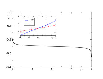
Figure 2: (Color online) Local response $\chi_{m}$ for a one-dimensional tight-binding chain as a function of the chemical potential $\mu$ for $\varepsilon_{m}=0$. The inset shows the ground state local density $n_{m}$ (red, dashed) and the total response density $n^{\rm tot}_{m}$ (blue, solid) as in Eq. (7).

Magnetic experiment. We develop the magnetic case by a gedanken experiment as far as possible in parallel with the above, aiming at a definition of the ring current that corresponds to Eq. (7). While the leads are biased and the current flows, we switch a weak uniform magnetic field of strength $B$ forming an angle $\theta$ with respect to the normal of the ring. We denote with $\phi$ the magnetic flux through the ring and with $|\Psi(\phi)\rangle$ the current carrying state of the system after all transient effects have disappeared. The derivative of the total energy $E(\phi)=\langle\Psi(\phi)|\hat{H}(\phi)|\Psi(\phi)\rangle$ would give the torque acting on the whole system. As in the electrostatic experiment, the wave function is modified everywhere even though the magnetic perturbation is localized and hence $\langle\Psi(\phi)|\mbox{$\hat{H}$}(\phi)-\mbox{$\hat{H}$}_{\rm ring}(\phi)|\Psi(\phi)\rangle$ depends on the flux and the external circuit experiences a torque as well. A further problem in using the variation of the total energy is related to the choices of the Peierls phases along the ring. The definition of the local torque should only depend on the magnetic flux $\phi=\alpha_{ab}+\alpha_{bc}+\alpha_{ca}$ through the ring. However, one can easily realize that the choice $\alpha_{ab}=\phi$ and $\alpha_{bc}=\alpha_{ca}=0$ (c1) and the choice $\alpha_{ab}=\alpha_{bc}=0$ and $\alpha_{ca}=\phi$ (c2), see Fig. 3, are not related via a gauge transformation and hence lead to different derivatives of the total energy with respect to $\phi$. The asymptotic current-carrying eigenstatenoi of $H$ can be used in both cases to invoke the Hellmann-Feynman theorem. The choice c1 then leads to the bond current $J_{ab}$ while the choice c2 to $J_{ca}$. The use of the total energy to calculate the torque experienced by the ring is therefore ambiguous. Next, we show that a local measurement on the ring is much more rewarding.

The ring interacts with the magnetic field and its energy relative to the chemical potential $\mu$ is

$$E_{\rm ring}(\phi) = \langle\Psi(\phi)|\mbox{$\hat{H}$}_{\rm ring}(\phi)-\mu\hat{N}_{\rm ring}|\Psi(\phi)\rangle$$ (8)

$$= -MB\cos\theta=-M\frac{\phi}{S},$$

where $\hat{N}_{\rm ring}$ is the number operator of the ring, $S$ is the ring surface and $M$ is the ring magnetic moment. We have no information about $S$, however, we may say that

$$\frac{1}{c}I_{\rm ring}=-\frac{M}{S}=\frac{dE_{\rm ring}}{d\phi}|_{\phi=0}.$$ (9)

The definition of the ring current does not suffer from the ambiguity originating from different possible choices of the Peierls phases. This follows from the fact that the operator $\mbox{$\hat{H}$}_{\rm ring}(\phi)-\mu\hat{N}_{\rm ring}$ is a local operator and hence its average only depends on the projection onto the ring of the single particle states $\{\psi_{k}\}$ forming the Slater determinant $|\Psi(\phi)\rangle$. Let us discuss this crucial point in more detail. We consider the choice c1 and let $\psi_{k}(m)$ be the amplitude on site $m$ of the $k$-th one-particle eigenstate of the total Hamiltonian, see Fig. (3). Similarly we denote with $\tilde{\psi}_{k}(m)$ the one-particle eigenstate corresponding to the choice c2. The choice c2 can be transformed in a gauge equivalent phase configuration (choice c2^′) in which the Peierls phases along the ring are the same as those in c1 but in the right lead there is a bond, e.g., the bond $1-2$, that acquires a phase $-\phi$. The eigenstate $\tilde{\psi}_{k}(m)$ of choice c2 is transformed in the eigenstate $\tilde{\psi}^{\prime}_{k}(m)$ accordingly. It is straightforward to realize that $\tilde{\psi}^{\prime}_{k}(m)=e^{i\frac{\phi}{c}}\psi_{k}(m)$ for $m>1$ while $\tilde{\psi}^{\prime}_{k}(m)=\psi_{k}(m)$ otherwise. As a consequence the average of the local operator $\mbox{$\hat{H}$}_{\rm ring}(\phi)-\mu\hat{N}_{\rm ring}$ over the gauge inequivalent configurations c1 and c2 does not change. Such result is independent of the choice of the Peiers phases along the ring provided that $\alpha_{ab}+\alpha_{bc}+\alpha_{ca}=\phi$.

Figure 3: Configuration of the Peierls phases along the bonds of the system. For choice c1 the phase is localized on the bond $a-b$ while for choice c2 the phase is along the bond $a-c$. Starting from c2, the multiplication of the fermion operators on sites $c$, $b$, and $-1$ by $e^{i\phi}$ is a gauge transformation which corresponds to the configuration c2^′.

Results and discussion. To calculate the ring current from Eq. (9) we use an embedding technique. We consider the system of Fig. 1 with zero on site energies everywhere and hopping $|t|$ between the sites connected by a link. Let $U_{L/R}$ be the bias applied to the left/right lead and $h$ be the matrix of the one-body operator $\mbox{$\hat{H}$}_{\rm ring}(\phi)=\sum_{ij}h_{ij}(\phi)c^{{\dagger}}_{i}c_{j}$. Then the average $E_{\rm ring}(\phi)$ in Eq. (8) can be expressed in terms of the lesser Green’s function $G^{<}$ as

$$E_{\rm ring}(\phi)=-i\int\frac{d\omega}{2\pi}{\rm Tr}_{\rm ring}\left[(h-\mu)G^{<}(\omega)\right],$$ (10)

where the trace is taken over the sites of the ring. The matrix $G^{<}(\omega)$ is the Fourier transform of the lesser Green’s function $G^{<}(t,t^{\prime})$ for times $t,t^{\prime}\rightarrow\infty$ and can be written as $G^{<}(\omega)=G^{\rm R}(\omega)[\Sigma^{<}_{L}(\omega)+\Sigma^{<}_{R}(\omega)]G^{\rm A}(\omega)$. The retarded/advanced Green’s function projected onto the ring is $G^{\rm R/A}(\omega)=[\omega-h-\Sigma^{\rm R/A}(\omega)]^{-1}$ with $\Sigma^{\rm R/A}=\Sigma^{\rm R/A}_{L}+\Sigma^{\rm R/A}_{R}$ the retarded/advanced embedding self-energy of the left and right leads. Using the fluctuation-dissipation theorem for lead $\alpha=L,R$ one obtains for the lesser embedding self-energy $\Sigma^{<}_{\alpha}(\omega)=-2if(\omega-U_{\alpha}){\rm Im}[\Sigma^{\rm R}_{\alpha}(\omega)]$, where $f(\omega)$ is the Fermi distribution function at chemical potential $\mu$. The retarded and advanced components are related as $\Sigma^{\rm R}_{\alpha}=[\Sigma^{\rm A}_{\alpha}]^{{\dagger}}$ with $\alpha=L,R$. For one-dimensional tight-binding leads with nearest neighbor hopping $t$ the self-energies have only one nonvanishing matrix element, namely $[\Sigma^{\rm R}_{L}(\omega)]_{ij}=\delta_{ia}\delta_{ja}\sigma(\omega-U_{L})$ and $[\Sigma^{\rm R}_{R}(\omega)]_{ij}=\delta_{ib}\delta_{jb}\sigma(\omega-U_{R})$. The function $\sigma(\omega)$ can be easily calculated and reads

$$\sigma(\omega)=\frac{1}{2}\left((\omega+i\eta)-\frac{(\omega+i\eta)+2t}{\sqrt{1+\frac{4t}{(\omega+i\eta)-2t}}}\right).$$ (11)

The ring current in Eq.(9) is obtained by taking the flux derivative of $E_{\rm ring}(\phi)$ in Eq. (10) in $\phi=0$. The flux derivative of the one-body matrix hamiltonian $h$ yields a linear combination of the one-body matrix bond currents with coefficients $\alpha_{ab}/\phi$, $\alpha_{bc}/\phi$ and $\alpha_{ca}/\phi$. This term alone would then be dependent on the Peierls phase configuration. The independence of $I_{\rm ring}$ from the phase configuration is restored by adding the flux derivative of $G^{<}(\omega)$ which reads

$$\frac{d}{d\phi}G^{<}=G^{\rm R}\left(\frac{dh}{\delta\phi}G^{\rm R}\Sigma^{<}+\Sigma^{<}G^{\rm A}\frac{dh}{d\phi}\right)G^{\rm A}.$$ (12)

Thus $I_{\rm ring}$ can be expressed in terms of $\frac{dh}{d\phi}|_{\phi=0}$ and Green’s functions at $\phi=0$. We wish to emphasize that for $\phi=0$ the ring current has no diamagnetic contribution.

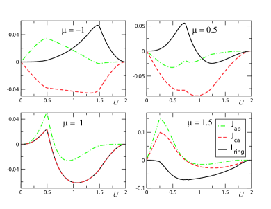
Figure 4: (Color online) Plot of the bond currents $J_{ab}$ (green, dot-dashed) and $J_{ca}$ (red, dashed) and of the ring current $I_{\rm ring}$ (black, solid) defined in Eq. (9) as a function of the applied bias voltage $U_{R}=-U_{L}=U$ for different values of the equilibrium chemical potential $\mu$. Energies are in units of the hopping parameter $t$ and currents are in units of $tG_{0}$ with $G_{0}$ the quantum of conductance.

In Fig. 4 we display the I/V characteristic of the ring current as well as of the bond currents along the $a-b$ and $c-a$ bonds for different values of the chemical potential $\mu=-1.5,0.-1.0,0.5,1.0$ in units of $t$. The bond-currents are computed using a Landauer-like formula derived in Ref. noi, . In all cases the ring current is quadratic in $U$ for small $U$ meaning that the ring conductance is always zero.

On the contrary, the bond currents are generally linear in $U$ except for special values of $\mu$ at which the bond conductance vanishes noi . One of these special values of $\mu$ is $\mu=1$. In this case the ring current coincides with the bond current along the $c-a$ bond for all values of $U$. We also observe that $I_{\rm ring}$ has a maximum as a function of $U$ and that the position of the maximum shifts towards high bias by increasing the chemical potential. For negative $\mu$ the maximum is located in correspondence of the maximum of the bond currents while for positive $\mu$ is locate in correspondence of their minimum. All currents correctly vanish for bias $U=2$ as the left continuum is lifted by 2 while the right continuum is lowered by the same amount. Since the bandwidth is 4 the bias $U=2$ represents the minimum value of $U$ for which there is no overlap between the left and right continua.

In a similar way one can compute $I_{\rm ring}$ for rings with $N$ sites, arms of different length and different hopping as well as onsite energy parameters. We have verified that $I_{\rm ring}=0$ for rings symmetrically connected, as physically expected.

In conclusion we have pointed out that for quantum circuits containing closed loops the theory of quantum transport needs to be extended in order to compute the loop magnetic moments which couple to an external magnetic field. By a suitable gedanken experiment we have been able to define a ring current which is independent of the Peierls phase configuration provided that $\alpha_{ab}+\alpha_{bc}+\alpha_{ca}=\phi$ is kept constant. The explicit calculation of $I_{\rm ring}$ in a ring connected to one-dimensional tight-binding leads show that $I_{\rm ring}$ is, in general, not given by a linear combination of the bond currents, even though there are common features. Our procedure differs from the one of Ref. matthias where the magnetic moment is obtained by an average over the bond currents. We believe that our treatment can be compared with experiment by measuring the ring magnetic moments, and paves the way to include induction and self-induction effects in quantum transport theory. In the extended theory, even in the absence of an external magnetic field one will need to consider a flux $\phi=cLI_{\rm ring}$ where $L$ is the self-induction coefficient.

References

- (1) R. Landauer, IBM J. Res. Dev. 1, 233 (1957).
- (2) C. Caroli, R. Combescot, P. Nozieres and D. Saint James, J. Phys. C 4, 916 (1971).
- (3) In this work we will use atomic units and spin indices will be omitted.
- (4) M. Cini, Phys. Rev. B 22, 5887 (1980).
- (5) M. Büttiker, Phys. Rev. Lett. 57, 1761 (1986).
- (6) H. Haug and A.-P. Jauho, Quantum Kinetics in Transport and Optics of Semiconductor, (Springer-Verlag, Berlin, 2008).
- (7) Michele Cini, Topics and Methods in Condensed Matter Theory, Springer Verlag (2007).
- (8) V. Chandrasekhar, R. A. Webb, M. J. Brady, M. B. Ketchen, W. J. Gallagher and A. Kleinsasser, Phys. Rev. Lett. 70, 2020 (1993); D. Mailly, C. Chapelier and A. Benoit, Phys. Rev. Lett. 67, 3578 (1991); H. Bluhm, N. C. Koshnick, J. A. Bert, M. E. Huber and K. A. Moler, Phys. Rev. Lett. 102, 136802 (2009).
- (9) F. Guinea, Phys. Rev. B 65 205317 (2002)
- (10) See, for instance, Quantum Transport: Persistent Current in Mesoscopic Loops, S. K. Maiti, arXiv:0706.0061v3, and references therein.
- (11) Molecular Electronics, edited by G. Cuniberti, G. Fagas, and K. Richter (Springer, Berlin, 2005).
- (12) J. Yi, G. Cuniberti, and M. Porto, Eur. Phys. J. B 33, 221 (2003).
- (13) M. Ernzerhof, H. Bahmann, F. Goyer, M. Zhuang and P. Rocheleau, J. Chem. Th. Comput. 2, 1291 (2006).
- (14) B. T. Pickup and P. W. Fowler, Chem. Phys. Lett. 459, 198 (2008).
- (15) A. M. Jayannavar and P. Singha Deo, Phys. Rev. B 51, 10175 (1995).
- (16) G. Stefanucci, E. Perfetto, S. Bellucci and M. Cini, Phys. Rev B 79, 073406 (2009).
- (17) W. Kohn, Phys. Rev. 133, A171 (1964).
- (18) A. Callegari, M. Cini , E. Perfetto, and G. Stefanucci, Eur. Phys. J. B 34, 455 (2003).