A Pulsational Mechanism for Producing Keplerian Disks around Be Stars

Abstract

Classical Be stars are an enigmatic subclass of rapidly rotating hot stars characterized by dense equatorial disks of gas that have been inferred to orbit with Keplerian velocities. Although these disks seem to be ejected from the star and not accreted, there is substantial observational evidence to show that the stars rotate more slowly than required for centrifugally driven mass loss. This paper develops an idea (proposed originally by Hiroyasu Ando and colleagues) that nonradial stellar pulsations inject enough angular momentum into the upper atmosphere to spin up a Keplerian disk. The pulsations themselves are evanescent in the stellar photosphere, but they may be unstable to the generation of resonant oscillations at the acoustic cutoff frequency. A detailed theory of the conversion from pulsations to resonant waves does not yet exist for realistic hot-star atmospheres, so the current models depend on a parameterized approximation for the efficiency of wave excitation. Once resonant waves have been formed, however, they grow in amplitude with increasing height, steepen into shocks, and exert radial and azimuthal Reynolds stresses on the mean fluid. Using reasonable assumptions for the stellar parameters, these processes were found to naturally create the inner boundary conditions required for dense Keplerian disks, even when the underlying B-star photosphere is rotating as slowly as 60% of its critical rotation speed. Because there is evidence for long-term changes in Be-star pulsational properties, this model may also account for the long-term variability of Be stars, including transitions between normal, Be, and shell phases.

1. Introduction

Be stars are non-supergiant B-type stars that exhibit emission in their hydrogen Balmer lines. It has been known for many decades (e.g., Struve 1931) that the “classical” Be stars tend to rotate more rapidly than normal non-emission B stars. A wide range of observations of Be stars is consistent with the coexistence of a dense circumstellar disk in the equatorial plane and a variable stellar wind at higher latitudes (Doazan 1982; Slettebak 1988; Prinja 1989; Porter & Rivinius 2003). There is a great deal of evidence that the so-called decretion disk is ejected from the star and is not accreted from an external source of gas. The physical mechanisms that are responsible for producing the disk, though, are still not known. This paper investigates the idea that nonradial pulsations (NRP) may deposit sufficient angular momentum above the photospheres of rapidly rotating Be stars to explain the origins of dense equatorial disks.

Theoretical explanations for the Be phenomenon depend crucially on how rapidly the stars and disks are rotating. Although there is increasing evidence that the extended disks are in Keplerian orbit (e.g., Hanuschik 1996; Hummel & Vrancken 2000; Okazaki 2007), there is also evidence to show that the underlying photospheres rotate too slowly to propel any atmospheric gas into orbit. Typical observational values of the ratio of equatorial rotation speed to the critical rotation speed $V_{\rm crit}$ (at which gravity is balanced by the outward centrifugal force) range between 0.5 and 0.8 (Slettebak 1982; Porter 1996; Yudin 2001). There has been some recent disagreement between this traditional picture and new ideas—inspired by the tendency for gravity darkening to mask rapid rotation at the equator—that most or all Be stars may be rotating very nearly at $V_{\rm crit}$ (Townsend et al.  2004). Cranmer (2005) found that this may be true for the late-type Be stars (i.e., spectral types B3 and later), but early-type Be stars do seem to be consistent with a range of intrinsic rotation speeds between $\sim$40% and 100% critical. For stars rotating sufficiently below $V_{\rm crit}$, any physical model for the origin of Be-star disks requires a significant increase in angular momentum above the photosphere.

This paper develops a set of ideas concerning how stellar NRP may give rise to outwardly propagating circumstellar waves, which in turn can deposit angular momentum in Be-star disks. The history of this theoretical perspective is discussed in more detail in § 2. However, a number of other disk formation mechanisms have been proposed, and it is important to keep in mind that in some cases these could be acting in cooperation or competition with the pulsational processes advocated here. Some of the other suggested mechanisms have been: (1) stellar “wind compression” that may channel supersonically outflowing gas from mid-latitudes to the equatorial plane by conservation of angular momentum (Bjorkman & Cassinelli 1993; Bjorkman 2000), (2) episodic ejections from some point on the star, with some material being propelled forward into orbit and some propelled backward to fall onto the star (Kroll & Hanuschik 1997; Owocki & Cranmer 2002), and (3) magnetic forces that can channel gas toward the equatorial plane and provide sufficient torque to spin up a disk (e.g., Poe & Friend 1986; Cassinelli et al.  2002; Brown et al.  2004, 2008; Ud-Doula et al.  2008).

The three mechanisms listed above have one general feature in common: they depend on the existence of large-scale supersonic flows in the circumstellar regions. Thus, these processes appear likely to give rise to strong variability on short (dynamical) time scales. Although many Be stars do exhibit variability on time scales of hours to days, many other Be stars seem to maintain their disks in a relatively quiescent manner over several years (see, e.g., Dachs 1987; Telting 2000; Okazaki 2007). It is worthwhile, then, to first consider a “baseline” disk formation mechanism that feeds the disk with a more or less steady-state supply of angular momentum from below. Other proposed mechanisms then may act as sources for the complex observed patterns of Be-star variability (see also § 6.2).

The outline of this paper is as follows. § 2 presents an overview of how stellar pulsations may be coupled to the outward transport of mass and momentum in the circumstellar regions of Be stars. In § 3 the detailed properties of waves and shocks are presented, including how evanescent pulsation modes couple to propagating waves, how these waves steepen into dissipative shocks, and how the waves can exert a net pressure to affect the time-steady properties of the stellar atmosphere. § 4 describes the time-independent conservation equations for mass and momentum that are solved with contributions from the waves, and § 5 gives the results. A discussion of the implications of these models on our overall understanding of Be-star disk formation and time variability is given in § 6. Finally, § 7 contains a brief summary of the major results and discusses how the proposed physical processes should be further tested and refined.

2. The Disk-Pulsation Connection

Do stellar pulsations represent a causal factor in producing the wide variety of observed manifestations of the Be phenomenon? This possible connection has been discussed for several decades both from the standpoints of Be-star observations (e.g., Baade 1982, 1985; Henrichs 1984; Willson 1986; Smith 1988) and pulsation theory (Ando 1986; Osaki 1986; Castor 1986; Saio 1994; Lee 2006, 2007). For a while, there was significant debate over whether much of the observed Be-star line profile variability was even the result of NRP, or if these features were simply rotationally modulated “spots” (e.g., Baade & Balona 1994). However, recent improvements in the detection and modeling of NRP in many Be stars has put the pulsational interpretation on firmer footing (Rivinius et al.  2003; Rivinius 2007; Townsend 2007).

The well-studied Be star $\mu$ Cen has been a key target in the search for disk-pulsation correlations (e.g., Rivinius et al.  1998). The multiple NRP periods of $\mu$ Cen seem to undergo beating in phase with outbursts of circumstellar material into the disk, suggesting a direct input of mass and momentum when the pulsation displacements are largest. Increases in disk emission at NRP amplitude maxima have also been observed for other multiperiodic Be stars such as $\zeta$ Oph (Kambe et al.  1993a) and 28 Cyg (Tubbesing et al.  2000). However, similar kinds of outbursts are also seen for Be stars like $\omega$ CMa that seem to have only a single pulsation period (Štefl et al.  2003). For other Be stars, there has been line profile variability observed at Doppler velocities that exceed the projected photospheric rotation velocity (Chen et al.  1989; Kambe et al.  1993b). This may be evidence for a radial increase in the rotation rate between the photosphere and the inner edge of the disk.

In addition to observational connections between pulsations and disks, there are many stars without disks (O, B, and Wolf-Rayet) for which there exists coupled variability between the photosphere and the stellar wind. The radial pulsator BW Vul clearly shows nonlinear shock-like features in its photosphere (e.g., Smith & Jeffery 2003) that are in phase with radially accelerating features in its supersonic wind (Massa 1994; Owocki & Cranmer 2002). Several stars show different periods for photospheric and wind variability, with the former (due to NRP) often being shorter than the latter (e.g., Howarth et al.  1993, 1998; Kaufer et al.  2007). Although much of the observed stellar wind variability may be attributed to structures corotating with the star (Kaper et al.  1996), the distribution of these stars in luminosity and effective temperature seems to agree roughly with the domain of so-called “strange-mode” oscillations (Fullerton et al.  1996), indicating that there may be a pulsational cause for some types of wind variability.

From a theoretical standpoint, it has been known for some time that small-scale hydrodynamic fluctuations (waves, shocks, turbulence, pulsations) can affect the large-scale mean properties of a fluid. Linear waves propagating in an inhomogeneous medium exert a time-steady wave pressure on the fluid even without dissipating (Bretherton & Garrett 1968; Dewar 1970; Jacques 1977). Alfvén wave pressure is believed to be a key contributor to the acceleration of the high-speed solar wind (e.g., Cranmer 2004). A nonlinear extension of this effect is likely to be acting in the outer atmospheres of cool pulsating giants and supergiants—e.g., Mira variables and asymptotic giant branch stars—with pulsation driven mass loss suspected to occur in many cases (Willson 2000; Woitke 2007; Neilson & Lester 2008).

In addition to supplying linear momentum, it has been shown that waves can transport and deposit angular momentum in rotating systems. Interior gravity waves in rotating planetary atmospheres have been shown to be responsible for driving various kinds of mean shear flows (Eliassen & Palm 1960; Bretherton 1969; Plumb 1977; Schatzman 1993; Rogers et al.  2008). In stellar interiors, the study of how diffusive transport processes interact with the mean rotation profile has proceeded with the implicit assumption that waves or turbulent eddies may be the cause of the “anomalous” transport (e.g., Rüdiger 1977; Zahn et al.  1997; Talon 2008). Ando (1982) considered the coupling between waves and rotation as a possible means of generating differential rotation in stellar interiors. Recently, Townsend & MacDonald (2008) found that the interior transport of angular momentum by pulsations may be an important factor in the evolution of rotating massive stars.

The application of the above ideas to the episodic spinup and mass loss of Be stars was developed by Ando (1986, 1988), Osaki (1986, 1999), Lee & Saio (1993), Saio (1994), and Lee (2006, 2007). This mechanism was originally believed to transport angular momentum up to the stellar surface only for prograde NRP modes (i.e., modes for which the azimuthal group velocity is in the same direction as the mean rotation); see, e.g., Ando (1983). A retrograde oscillation mode was thought to transport angular momentum downward and thus potentially spin down the outer layers of the star. However, more recent work—which takes a more complete inventory of the various second order wave-rotation coupling terms—finds that some types of coupling do not depend at all on the sign of the azimuthal group velocity (e.g., Lee 2007). Furthermore, Townsend (2005) and Pantillon et al.  (2007) showed that some “mixed modes” may exist in rapidly rotating stars that appear to have retrograde phase velocities but prograde group velocities. There are thus several potential ways for retrograde NRP modes (which appear to be prevalent in Be stars) to be associated with the transport of angular momentum up to the surface and beyond.

Aside from the work of Ando and colleagues, though, surprisingly little work has been done to study how pulsational energy (as well as the effects of pulsations on the mean fluid) may “leak” out of a hot star into its circumstellar medium. Cranmer (1996) studied some aspects of how low-frequency evanescent waves in B-star photospheres might evolve into propagating waves at larger heights in a stellar wind. Townsend (2000a,b,c) modeled NRP leakage from the perspective of whether the $p$ and $g$ modes are propagating or evanescent in the layers directly beneath the photosphere (see also Gautschy 1992). The goal of this paper is to follow up on these ideas and to investigate how an extended hot-star atmosphere responds to the presence of pulsational oscillations at its photospheric base.

3. Waves and Shocks

This section contains a derivation of some of the physical processes that determine how pulsationally driven waves can influence the mean properties of a stellar atmosphere. The subsections below isolate four of the main effects that need to be considered: evanescence (§ 3.1), resonant excitation at the acoustic cutoff (§ 3.2), shock steepening and dissipation (§ 3.3), and wave pressure (§ 3.4). Some of the proposed connections between the above mechanisms are still somewhat speculative, so it is hoped that this combination of ideas will eventually be tested with numerical simulations.

This paper makes the implicit assumption that there is a reasonably time-steady input stream of pulsational oscillations from the stellar interior. Observations suggest, however, that many NRP modes have finite lifetimes, and that they undergo secular amplitude variations over a wide range of time scales (see § 6.2 for discussion of the implications of NRP transience on Be-star variability). The models presented below also ignore several effects that may be important in some situations, such as heat conduction, radiative damping, magnetic fields, and ballistic freefall behind strong shocks (the latter being important in, e.g., Mira variables).

3.1. Evanescent Pulsation Modes

For the purposes of modeling the effects of B-star NRP oscillations on their outer atmospheres, it is important to first summarize what is known about them observationally. The $\beta$ Cep variables have typical pulsation periods of order 2–10 hrs, spectral types between B0 and B2, and are often interpreted as low-order $p$ and $g$ modes (Sterken & Jerzykiewicz 1992; Aerts & de Cat 2003). Slowly pulsating B (SPB) stars have longer periods of 10–50 hrs, later spectral types of B3 to B9, and they appear to be pulsating in high-order $g$ modes (e.g., de Cat 2007). Pulsating Be stars often have periods that appear similar to the SPB class, but with some modes (including beat periods) that extend up into the 100–200 hr range (e.g., Kaufer et al.  2006). Some B stars are “hybrid” pulsators that exhibit both $\beta$ Cep and SPB type modes (Dziembowski & Pamyatnykh 2008).

Figure 1 shows a collection of B-star pulsation frequencies $\omega$ and horizontal wavenumbers $k_{x}$ that have been normalized, respectively, by dividing by an estimated acoustic cutoff frequency $\omega_{a}$ in the photosphere and multiplying by an estimated density scale height $H$. Spectral types, periods, and angular mode identifications were obtained for the $\beta$ Cep and SPB stars from de Cat (2002, 2003) and for Be stars from Rivinius et al.  (2003). Additional low-frequency modes for two hybrid B-type pulsators (12 Lac and $\nu$ Eri) were taken from Dziembowski & Pamyatnykh (2008), and the assignment of $\ell=|m|=2$ to these modes is relatively uncertain.

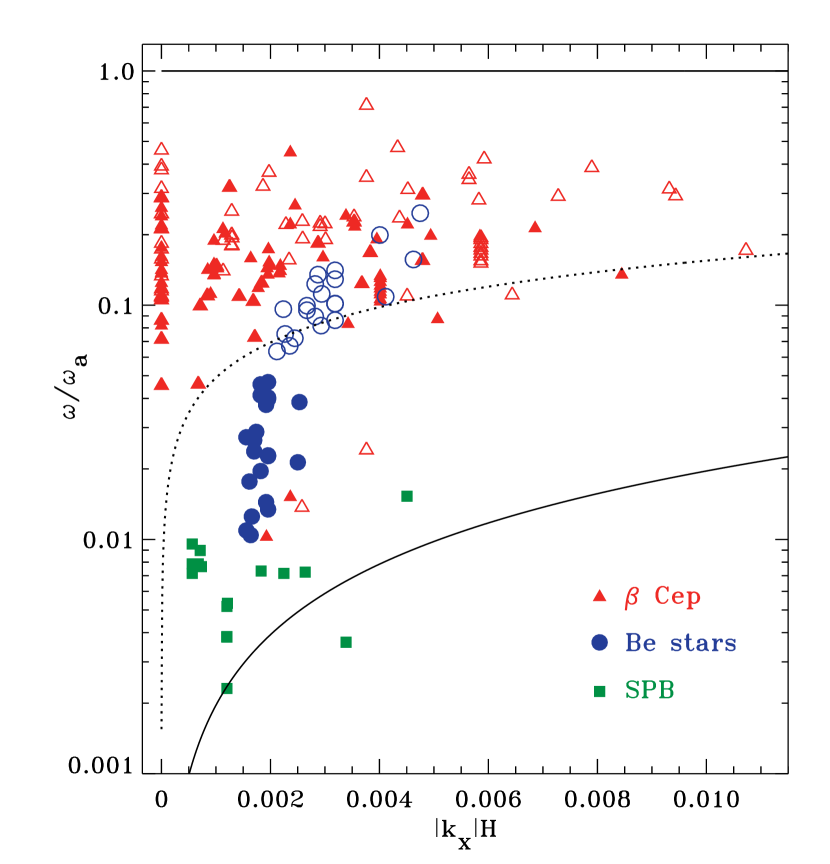
Figure 1.— Collected B-star pulsation frequencies and azimuthal wavenumbers, normalized to dimensionless quantities via the photospheric acoustic cutoff frequencies $\omega_{a}$ and scale heights $H$. Data for $\beta$ Cep variables (red triangles), SPB stars (green squares), and Be stars (blue circles) are shown. Filled symbols assume nonrotating stellar properties; open symbols attempt to take account of rapid rotation. Also shown are acoustic-gravity wave propagation boundaries (solid lines) and $f$-mode curve (dotted line).

The two-dimensional ($\omega,k_{x}$) plot illustrated by Figure 1 is often called a diagnostic diagram for waves in stellar atmospheres. The solid curves are the “propagation boundary curves” between which acoustic-gravity waves are evanescent. Above the upper curve, waves propagate vertically as acoustic or $p$-mode waves; below the lower curve, they propagate as internal gravity or $g$-mode waves (e.g., Lamb 1908, 1932; Mihalas & Mihalas 1984). To determine the normalizing values of the acoustic cutoff frequency $\omega_{a}$ and scale height $H$ for each star, the tabulated spectral types and luminosity classes were converted into stellar masses $M_{\ast}$, radii $R_{\ast}$, and effective temperatures $T_{\rm eff}$ in a single uniform way; i.e., using the luminosity and $T_{\rm eff}$ relations of de Jager & Nieuwenhuijzen (1987), and interpolating onto the evolutionary tracks of Claret (2004) to obtain masses (see also § 2 of Cranmer 2005). The magnitude of the horizontal wavenumber was computed from the tabulated meridional degree number $\ell$ and the assumption that $\ell=|m|$, the latter being the azimuthal mode number. Thus, $|k_{x}|=|m|/R_{\ast}$. For the Be stars, only the modes identified as having $m=2$ by Rivinius et al.  (2003) are shown.

The solid symbols in Figure 1 show values computed using the standard expressions for $\omega_{a}$ and $H$ for nonrotating stars (see below). The open symbols show modified values that take account of two attempts at improving the accuracy of these normalizations:

1. The surface gravity was reduced by taking account of both centrifugal and radiative acceleration. A lower limit to the stellar rotation was applied by assuming that the observed projected rotation rate $v\sin i$ is equal to the actual equatorial rotation speed $V_{\rm rot}$. For the Be stars, it was assumed that the rotation speed is never smaller than $V_{\rm crit}/2$ (see Cranmer 2005). The radiative acceleration in the photosphere was estimated using a fit to the numerical results of Lanz & Hubeny (2007) given by equations (31)–(32) below.

2. For the Be stars only, the observed pulsation frequency was replaced by an estimate of the intrinsic pulsation frequency in the rotating frame, assuming that the Be-star oscillations are retrograde (Rivinius et al.  2003). In this case, the rotating-frame frequency $\omega$ is higher than the observed inertial-frame frequency $\omega_{0}$, with

   $$\omega\,\approx\,\omega_{0}+m\Omega(1-C_{n\ell})$$ (1)

   and $C_{n\ell}\approx 0.2$ for low-order $f$ and $g$ modes (e.g., Ledoux 1951). We ignored second order centrifugal terms in the above expression (i.e., terms proportional to $\Omega^{2}/\omega$) since for low-order $g$ modes with $\ell=|m|=2$ they would give a negligibly small correction (Saio 1981).

For the SPB stars, these corrections were found to be unimportant and are not shown.

Taking account of the above effects results in smaller values of $\omega_{a}$ and in larger values of both $\omega$ and $H$, thus moving each data point upwards and to the right in Figure 1. Even with these corrections, though, nearly all of the observed pulsation modes are still solidly evanescent (i.e., not propagating vertically) in the photosphere. Also, the Be-star data points seem to have moved from the upper edge of the SPB region into the $\beta$ Cep region. (Many of them seem to cluster around the fundamental-mode curve, given by $\omega^{2}=gk_{x}$, which is a rough boundary between the $p$-mode and $g$-mode regions.) This may suggest that classical Be-star pulsations have a similar intrinsic character as those of the $\beta$ Cep variables, despite the apparent similarity of their periods to those of the SPB stars (see also Baade 1982).

The observed ranges of oscillation parameters can be put into context by using a theoretical model of acoustic-gravity waves. The model presented here makes the simplifying assumptions of an isothermal (constant temperature $T$) medium, plane-parallel geometry, and a constant gravitational acceleration $g$. It is also straightforward to first consider the system in the rotating frame, in which we define the frequency $\omega$. In this atmosphere, the sound speed is constant and is given by

$$c_{s}\,=\,\sqrt{\frac{\gamma P_{0}}{\rho_{0}}}\,=\,\sqrt{\frac{\gamma k_{\rm B}T}{\mu m_{\rm H}}}\,\,,$$ (2)

where $k_{\rm B}$ is Boltzmann’s constant, $m_{\rm H}$ is the mass of a hydrogen atom, and $\mu$ is the mean molecular weight of the gas. The latter quantity is assumed to be $\mu=0.604$, which corresponds to a standard (10% helium) elemental abundance mixture. The adiabatic exponent $\gamma$ is the ratio of specific heats $c_{p}/c_{v}$, and usually can range between 1 (isothermal) and 5/3 (adiabatic). For an isothermal atmosphere, the pressure and density scale heights are equal to one another and given by $H=c_{s}^{2}/\gamma g$ (which does not depend on the value of $\gamma$ itself).

The standard assumption in linear wave theory is to model the physical variables (i.e., density, velocity, pressure) as the sum of a time-steady (zeroth order) component and an oscillating (first order) component. The linear amplitudes vary as $e^{i\omega t-ik_{z}z-ik_{x}x}$ with a real frequency $\omega$. We model the conditions in the equatorial plane, with gravity acting in the $-z$ direction and the stellar rotation proceeding in the $+x$ direction (see Appendix). The azimuthal wavenumber can thus be expressed in conventional NRP terminology as $k_{x}=-m/R_{\ast}$, with negative [positive] values of $m$ corresponding to prograde [retrograde] modes. The time-steady vertical velocity $w_{0}$ is assumed to be zero, and the azimuthal velocity $u_{0}$ is also set to zero (in the rotating frame). The zeroth-order density $\rho_{0}$ is proportional to $e^{-z/H}$. The corresponding linear amplitudes are denoted $w_{1}$, $u_{1}$, and $\rho_{1}$, and they are modeled as complex quantities in order to account for phase differences between their respective oscillations.

For a given frequency $\omega$ and horizontal wavenumber $k_{x}$, the vertical wavenumber is in general a complex quantity given by

$$k_{z}\,=\,\frac{i}{2H}\pm\left[\frac{(\omega^{2}-\omega_{a}^{2})}{c_{s}^{2}}-\frac{(\omega^{2}-\omega_{g}^{2})\,k_{x}^{2}}{\omega^{2}}\right]^{1/2}\,\,,$$ (3)

where the acoustic cutoff frequency is $\omega_{a}=\gamma g/2c_{s}$ and the Brunt-Väisälä frequency is $\omega_{g}=(\gamma-1)^{1/2}g/c_{s}$ (see, e.g., Lamb 1932; Mihalas & Mihalas 1984; Wang et al.  1995). The regions of $(\omega,k_{x})$ space where the vertical wavenumber has a real part correspond to propagating waves, and the regions where $k_{z}$ is completely imaginary correspond to evanescence. If the amplitude and phase of the vertical velocity amplitude $w_{1}$ are specified, the horizontal velocity and density fluctuations are given in dimensionless form by

$$\frac{u_{1}}{w_{1}}\,=\,\frac{c_{s}^{2}k_{x}}{\omega^{2}-c_{s}^{2}k_{x}^{2}}\left(k_{z}-\frac{i}{\gamma H}\right)$$ (4)

$$\frac{\rho_{1}/\rho_{0}}{w_{1}/c_{s}}\,=\,\frac{\omega c_{s}}{\omega^{2}-c_{s}^{2}k_{x}^{2}}\left\{k_{z}+\frac{i}{H}\left[\frac{(\gamma-1)c_{s}^{2}k_{x}^{2}}{\gamma\omega^{2}}-1\right]\right\}\,\,.$$ (5)

Note that when $k_{z}$ is completely imaginary, the above expressions are also imaginary. This implies that in the case of evanescent waves, $u_{1}$ and $w_{1}$ are 90° out of phase, and $\rho_{1}$ and $w_{1}$ are also 90° out of phase.

It is useful to illustrate how these waves behave in the limit of small horizontal wavenumbers (i.e., $|k_{x}H|\ll 1$) which applies to B-star NRP observed at the stellar surface (see Figure 1). It is also useful to use the simplifying limit of $\gamma=1$, which corresponds to isothermal fluctuations. This approximation is consistent with the existence of rapid radiative heating and cooling in the relatively dense outer atmospheres of hot O and B stars (e.g., Drew 1989; Millar & Marlborough 1999; Carciofi & Bjorkman 2006). With the above assumptions, the lower propagation boundary disappears and the upper propagation boundary is greatly simplified: i.e., waves with $\omega>\omega_{a}$ propagate; waves with $\omega<\omega_{a}$ are evanescent.

Propagating waves have exponentially growing amplitudes with height, with the non-oscillating part of the height dependence being given by $w_{1}\propto e^{z/2H}$. These waves have a vertical phase speed

$$V_{\rm ph}\,=\,\frac{\omega}{\mbox{Re}\,k_{z}}\,\approx\,c_{s}\left(1-\frac{\omega_{a}^{2}}{\omega^{2}}\right)^{-1/2}$$ (6)

and a group velocity $V_{\rm gr}=c_{s}^{2}/V_{\rm ph}$. For upwardly propagating waves, the above amplitude relations can be simplified to show that

$$\mbox{Re}\left(\frac{u_{1}}{w_{1}}\right)\,\approx\,2k_{x}H\,\frac{\omega_{a}}{\omega}\,\frac{c_{s}}{V_{\rm ph}}\,\ll 1$$ (7)

$$\mbox{Re}\left(\frac{\rho_{1}/\rho_{0}}{w_{1}/c_{s}}\right)\,\approx\,\frac{c_{s}}{V_{\rm ph}}\,\,.$$ (8)

Note that the sign of $k_{x}$ determines the sign of the magnitude ratio $u_{1}/w_{1}$, but the ratio $\rho_{1}/w_{1}$ is positive definite.

Evanescent waves have two possible solutions for their (completely non-oscillatory) height dependence; one “steeper” than the propagating solution, and one “shallower.” The shallow [steep] solution has a total wave energy density that decays [grows] with increasing height. Thus, the shallow solution is the physically realistic choice when considering waves that originate at low heights and have effects on the medium at larger heights (see, e.g., Wang et al.  1995). The vertical amplitude dependence of the shallow solution is given by

$$w_{1}\,\propto\,\exp\left[\frac{z}{2H}\left(1-\sqrt{1-\frac{\omega^{2}}{\omega_{a}^{2}}}\right)\right]\,\,.$$ (9)

For evanescent waves, the phase speed is formally infinite and the group velocity is zero. However, Cranmer (1996) showed that if a time-steady subsonic wind ($w_{0}\ll c_{s}$) is included in the linear equations for acoustic-gravity waves, the shallow evanescent solution can be shown to have a large—but finite—upward phase speed of order $c_{s}^{2}/w_{0}$. The steep evanescent solution corresponds to a downward phase speed of $-c_{s}^{2}/3w_{0}$. These both correspond to negligibly small (subsonic) group velocities and do not need to be considered further.

3.2. Resonant Wave Excitation

It has been known for some time that the acoustic cutoff $\omega_{a}$ is a preferred resonance frequency for an atmosphere that has been disturbed by a pulse or piston-like initial condition (see, e.g., Lamb 1908; Schmidt & Zirker 1963). The acoustic cutoff frequency also acts as a fundamental “ringing” mode for disturbances of a sinusoidal nature (Fleck & Schmitz 1991; Kalkofen et al.  1994; Sutmann et al.  1998). Of particular interest here is the case of an evanescent oscillation driven by NRP (with $\omega<\omega_{a}$) that can excite a resonant oscillation ($\omega\approx\omega_{a}$).

The one-dimensional problem of resonant excitation in an infinite isothermal atmosphere can be solved analytically (e.g., Fleck & Schmitz 1991). In this section we make use of this simple model to gain insight about the physics of resonant waves. Although the model contains features that are formally inapplicable to actual pulsating stars (i.e., the assumption of an instantaneous “start” at $t=0$), it remains valuable as a way to obtain numerical estimates of the resonant wave properties in the absence of a more accurate theory. Let us then consider a piston with an average height slightly below the photosphere ($z_{\rm piston}<0$) with a vertical pulsation amplitude $V_{\rm puls}$. For simplicity, the long-wavelength horizontal velocity fluctuations can be ignored; i.e., $k_{x}=0$. Thus, for a piston oscillating with evanescent frequency $\omega$, the height dependence of this driven mode is given by equation (9), and its time dependence at larger heights remains strictly sinusoidal. In addition, when the piston motion begins (at time $t=0$) there arises a resonant response at the acoustic cutoff frequency. These two components of the vertical velocity amplitude can be expressed as

$$w_{1}(z,t)\,=\,V_{\rm puls}e^{-i\omega t+\kappa Z}\,\,+$$

$$V_{\rm res}(z,t)\left[\sin\left(\omega_{a}t-\frac{3\pi}{4}\right)+\frac{i\omega}{\omega_{a}}\cos\left(\omega_{a}t-\frac{3\pi}{4}\right)\right]$$ (10)

where $Z\equiv(z-z_{\rm piston})/2H$ and $\kappa=1-(1-\omega^{2}/\omega_{a}^{2})^{1/2}$ (Kalkofen et al.  1994; Sutmann et al.  1998). In the late-time limit of $t\gg z/c_{s}$, after which the initial transient disturbance has propagated away, the resonant component’s velocity amplitude is given by

$$V_{\rm res}(z,t)\,=\,V_{\rm puls}\sqrt{\frac{2\omega_{a}}{\pi}}\,\frac{Ze^{Z}}{(\omega_{a}^{2}-\omega^{2})\,t^{3/2}}\,\,.$$ (11)

This expression gives only the lowest order term in an infinite expansion; the higher order terms have more rapid time decay (e.g., $t^{-5/2}$, $t^{-7/2}$, etc.) and thus the above term dominates the late-time ($t\gg z/c_{s}$) behavior of the resonant mode.

For a given time $t$ after the piston begins to oscillate, both the driven (evanescent) mode and the resonant (cutoff) mode coexist in the atmosphere. Immediately above the piston, $V_{\rm res}\ll V_{\rm puls}$, but as one proceeds higher in the atmosphere, the radial growth of the resonant mode overtakes that of the shallow evanescent mode (eq. [9]) and the resonant mode becomes stronger. It is suspected that the stellar photosphere sits below the height where this transition occurs, because the observable signatures of NRP show only the evanescent driver. A major conjecture of this paper is that the upper layers of the atmosphere—including the “inner edge” of the Keplerian disk—are those where the resonant oscillations are dominant.

Equation (11) shows that the resonant oscillation amplitude decays in time as $t^{-3/2}$. If left undisturbed it would decay eventually to zero, leaving only the driven evanescent mode. However, this property of the solution seems to be an artifact of the idealized nature of an infinitely extended, isothermal, and plane-parallel atmosphere. For a real atmosphere, there are several effects that have been suggested to arrest this decay and produce a quasi-steady stream of resonant waves:

1. Fleck & Schmitz (1991) found that a sharp reflecting boundary at some height above the piston (even a relatively permeable one) can cause enough downward reflection of the resonant waves to maintain them at a finite amplitude over long times. Reflection effectively “restarts the clock” on the time $t$ in equation (11) every time the piston sees a reflected wave.

2. Radial gradients in the sound speed or scale height give rise to gradual linear reflection that can lead to continual excitation of the resonant waves (e.g., Pitteway & Hines 1965; Schmitz & Fleck 1992; Lou 1995; Musielak et al.  2005; Erdélyi et al.  2007; Taroyan & Erdélyi 2008). This kind of reflection is also believed to be acting on Alfvén waves in the solar chromosphere and corona, and in that case it may be responsible for seeding an ongoing turbulent cascade (Heinemann & Olbert 1980; Matthaeus et al.  1999; Cranmer & van Ballegooijen 2005).

3. If the driven evanescent oscillations are multiperiodic or stochastic in nature, the resulting departures from simple sinusoidal piston motion could result in continuously excited resonant waves. Such intermittency could be the result of rotationally generated subsurface convection (Espinosa Lara & Rieutord 2007; Maeder et al.  2008), NRP mode beating (Rivinius et al.  1998), or other nonlinear processes that can cause one NRP mode to grow at the expense of another mode (see, e.g., Smith 1986).

The remainder of this paper assumes the existence of a continual regeneration of resonant oscillations in B-star atmospheres. The general phenomenon of wave reflection seems to be the most likely route for this to occur. Fleck & Schmitz (1991) showed how the presence of wave reflection may cause the resonant waves to “forget” about an instantaneous initial condition and become essentially self-sustaining. Although the reflection in the models of Fleck & Schmitz (1991) was induced by a sharp upper boundary, there are several other ways that reflection can be produced gradually in an actual stellar atmosphere (see the second item in the above list). In the absence of a robust theory or simulation of these effects in hot-star atmospheres, however, we are limited to using simpler prescriptions such as equation (11).

The use of the simple theory derived above should not be interpreted as a suggestion that resonant waves are produced by an abrupt initial condition. This model is used only to estimate the mean amplitude of a steady-state ensemble of resonant waves, by choosing a representative time $t$ in equation (11). Equivalently, this can be specified in terms of the height $\Lambda$ of a fictional reflecting boundary above the photosphere, and the reflection time is thus estimated as $t\approx\Lambda/c_{s}$ (see, e.g., Figure 2 of Fleck & Schmitz 1991). The parameter $\Lambda$ is used as a free parameter in the models discussed below. Eventually, of course, there should be time-dependent numerical simulations of the partial wave reflection and resonant wave excitation in B-star atmospheres that would allow the most appropriate values of $\Lambda$ to be determined.

What values of $\Lambda$ should be considered realistic? It is useful to estimate the heights in the atmosphere at which the fluid parameters are thought to undergo qualitative changes. These are the heights at which substantial wave reflection should occur. One suggestion is to compute the height at which the strongest wave modes steepen into shocks (and probably saturate in amplitude). This onset of nonlinearity signals a rapid change in the overall properties of the atmosphere. For hot stars with NRP amplitudes that are already of the same order as the sound speed in the photosphere, the height at which they steepen into shocks may be as low as 2 to 4 photospheric scale heights above the photosphere itself. For a star with an accelerating wind, other significant heights would be the sonic and critical points (which are not the same for a radiatively driven wind; see Castor et al.  1975). For the standard B2 V star model discussed in detail in § 5, the sonic point would be at a radius of about 10 scale heights. The critical point is another scale height or two above the sonic point.

It is possible, though, that the relevant time scale $t$ could be much larger than suggested above. For a B star, a value of $\Lambda\approx 10H$ corresponds to a time that is only about 10% of a single evanescent NRP period. If $t$ is determined instead by long-term secular changes in the NRP “piston” (i.e., beating or mode growth/decay), it may be as large as the mode lifetimes themselves; typically no smaller than 10 to 100 NRP periods. However, since there is also evidence for shorter time scales being important (consistent with ongoing wave reflection from the upper atmosphere), we will make the order-of-magnitude assumption that $\Lambda$ is of order 10 scale heights and vary it up and down from that baseline value.

Figure 2 compares the height dependences of vertical velocity amplitudes for evanescent and resonant waves. The stellar parameters assumed here are those of the baseline B2 V model discussed in detail in § 5. The evanescent NRP driver has a period of 10 hrs, the acoustic cutoff period is 1.3 hrs, and the piston is assumed to sit $0.5H$ below the photosphere. For an assumed value of $\Lambda=10H$, the resonant mode becomes stronger than the evanescent mode at a height of approximately 4 scale heights above the photosphere (i.e., when the hydrostatic density has dropped by a factor of $\sim$50 from the photospheric value). Also shown is an upper-limit velocity amplitude $V_{\rm max}$ that illustrates the total energy density available for waves in a stratified atmosphere. This quantity was computed under the assumption that $\rho_{0}V_{\rm max}^{2}$ is constant, and $V_{\rm max}$ is normalized by the evanescent NRP driving amplitude at the piston. The thick curves show linear undamped solutions (i.e., eq. [11]) and the thin curves show the result of applying the shock steepening, dissipation, and wave pressure effects discussed below.

Figure 2.— Comparison of height dependences for driven evanescent wave amplitudes $V_{\rm puls}$ (dashed line), resonantly excited wave amplitudes $V_{\rm res}$ (solid lines), and the maximum available wave amplitudes $V_{\rm max}$ from energy conservation (dotted lines). Thick lines denote ideal linear results; thin lines show numerical results that take account of wave dissipation and shock steepening.

Note that the radial growth of the undamped resonant mode is more rapid than for a classical acoustic-gravity wave at $\omega\geq\omega_{a}$ (the latter illustrated by $V_{\rm max}\propto e^{Z}$). The extra linear factor of $Z$ in equation (11) is a unique feature of the resonantly excited oscillation. This factor has the strongest impact very near the piston height, but grows progressively less important once one goes a few scale heights above the piston. The resulting properties of the upper atmosphere are thus relatively insensitive to the exact value chosen for $z_{\rm piston}$. Also, when wave damping and wave pressure are taken into account (i.e., the thin curves in Fig.  2) the resonant mode no longer grows faster than $V_{\rm max}$ at all.

Choosing larger values of the reflection height $\Lambda$ results in a lower “efficiency” in the conversion of driving wave energy to resonant wave energy. This efficiency is estimated as the ratio $V_{\rm res}/V_{\rm max}$, and Figure 3 shows how this varies as a function of the $\Lambda$ parameter itself. The models that were used to compute these efficiencies contained the full range of shock steepening and wave pressure effects (see §§ 3.3–3.4), and they constrained $V_{\rm res}$ to never exceed the maximum available energy specified by $V_{\rm max}$. The efficiencies are shown both at the photospheric base and at the height of peak efficiency. The latter occurs usually a few scale heights above the photosphere, before substantial damping sets in. It is clear that values of $\Lambda/H$ less than about 3 or 4 may not be physically realistic, since they result in the resonant wave attempting to extract more energy from the driving mode than is actually available.

Figure 3.— Efficiency of resonant excitation ($V_{\rm res}/V_{\rm max}$) plotted as a function of the assumed reflection height $\Lambda$ for a series of B2 V atmosphere models (see text). The photospheric (dotted line) and maximum (solid line) values for each model are shown.

At the subphotospheric height of the idealized piston, the models below ignore the effects of radiative acceleration $g_{\rm rad}$ (which can counteract gravity at and above the photosphere). Lanz & Hubeny (2007) reported the existence of a local maximum in $g_{\rm rad}$ at the $\tau\approx 1$ photosphere, with less of an effect in the deeper layers that have smaller temperature gradients. Thus, because the net gravitational acceleration is higher at the piston than in the photosphere, the acoustic cutoff frequency at the piston is assumed to be slightly higher than that at the photosphere. For the standard B2 V star model, this results in a resonantly excited wave having a frequency about 1.2 times the local acoustic cutoff frequency once it reaches the photosphere. In other words, the assumption is that the wave eventually “forgets” about its origin as a resonant excitation and just propagates (as any other linear wave would) with a constant frequency.

3.3. Wave Action Conservation and Shock Dissipation

The resonantly excited wave modes discussed above ($\omega\gtrsim\omega_{a}$) are assumed to propagate upward from the photosphere and grow in amplitude. At some point, these mainly longitudinal fluctuations are expected to steepen into shocks and begin to dissipate some of their energy (e.g., Castor 1986). The nonlinear evolution of such a wave train is modeled here using a formalism described more completely by Cranmer et al.  (2007). The wave energy density $U_{s}$ is assumed to obey an equation of wave action conservation,

$$\frac{\partial}{\partial t}\left(\frac{U_{s}}{\omega^{\prime}}\right)+\frac{1}{A}\frac{\partial}{\partial z}\left[\frac{(w_{0}+V_{\rm gr})AU_{s}}{\omega^{\prime}}\right]\,=\,-\frac{Q_{\rm sh}}{\omega^{\prime}}$$ (12)

(see also Jacques 1977; Koninx 1992), where $A$ is the cross-sectional area of a flow tube and $Q_{\rm sh}$ is the shock dissipation rate. The time derivative term in equation (12) is given only for completeness and is ignored in the time-stationary models below. In general, the Doppler shifted frequency in the moving frame (i.e., taking account of both rotation and a stellar wind) is given by $\omega^{\prime}=\omega-u_{0}k_{x}-w_{0}k_{z}$. As above, the $u_{0}$ effect is ignored by interpreting $\omega$ as the corotating frequency, and the factor dependent on $w_{0}$ is taken into account by using the proper dispersion relation. The wave energy density is defined as

$$U_{s}\,=\,\frac{1}{s}\rho w_{1}^{2}$$ (13)

where $s$ is a dimensionless shape factor determined by the spatial profile of the waves. The peak-to-peak vertical velocity amplitude is denoted $w_{1}$, and the variance $w_{1}^{2}$ is equivalent to the magnitude of the product $w_{1}^{\ast}w_{1}$ (see Appendix).

The adopted area function $A(z)$ contains both the spherical expansion of the stellar atmosphere and an additional linear factor (depending on the distance above the piston) that describes how the resonantly excited waves differ from standard acoustic-gravity waves (eq. [11]). Thus,

$$A\,\propto\,\frac{r^{2}}{(z-z_{\rm piston})^{2}}$$ (14)

where $r$ is measured from the center of the star, and thus only varies by a few percent over the heights considered here. The models use the assumption that $z_{\rm piston}$ is $0.5H$ below the photosphere. Although $A$ diverges unphysically at $z=z_{\rm piston}$, this location is always kept outside the modeled grid of heights. The precise normalization of $A$ is unimportant, and only its relative variation with height enters into equations (12) and (15).

The Doppler shifted frequency $\omega^{\prime}$ can be computed in terms of the comoving-frame phase speed $V_{\rm ph}$, and a more useful version of the wave action conservation equation can be written as

$$\frac{\partial}{\partial r}\left[\frac{(w_{0}+V_{\rm gr})(w_{0}+V_{\rm ph})AU_{s}}{V_{\rm ph}}\right]\,=\,-\frac{(w_{0}+V_{\rm ph})AQ_{\rm sh}}{V_{\rm ph}}\,\,.$$ (15)

At the photospheric base, the lower boundary condition on the wave energy density is specified as $U_{s}=\rho V_{\rm res}^{2}/2$, with $s=2$ (i.e., a sinusoidal wave shape) also assumed at this height.

Before proceeding to describe the shock steepening in more detail, it is useful to examine the wave action equation in a simpler limiting case. For a negligibly small vertical wind speed $w_{0}$, and for waves sufficiently above the acoustic cutoff frequency that $V_{\rm ph}\approx V_{\rm gr}\approx c_{s}$, equation (15) simplifies greatly to become

$$c_{s}\frac{\partial U_{s}}{\partial r}\,=\,-Q_{\rm sh}\,\,,$$ (16)

where the additional assumption of $A\approx\mbox{constant}$ was also applied for large heights $z\gg z_{\rm piston}$ in a plane-parallel atmosphere. This equation has the benefit of clearly illustrating how shock dissipation affects the radial gradient of the wave energy density. The other terms that have been stripped away are non-dissipative contributors to the wave energy gradient. Although the numerical solutions presented in § 5 utilize the more complete equation of wave action conservation (eq. [15]), the simplified form of equation (16) is later found to be useful to derive a physically meaningful expression for the wave pressure.

A standard way of expressing the time-averaged shock dissipation rate is

$$Q_{\rm sh}\,=\,\frac{\rho T\Delta S}{2\pi/\omega}\,\,,$$ (17)

where $\Delta S$ is the net entropy jump across a shock, and it is nonzero only above the height where the wave train has steepened into shocks. This expression uses an approximation from so-called “weak-shock theory” that the volumetric heating rate is given by the internal energy dissipated at one shock divided by the mean time between shock passages in a periodic train. This assumption breaks down for very strong radiative shock trains (e.g., Carlsson & Stein 1992, 1997), which dissipate their energy in relatively narrow zones behind each shock. However, the models presented below do not develop such strong shocks. The gain in internal energy across an ideal inviscid shock is given by

$$T\Delta S\,=\,c_{v}\left[T_{2}-T_{1}\left(\rho_{2}/\rho_{1}\right)^{\gamma-1}\right]$$ (18)

where $c_{v}$ is the specific heat at constant volume for an ideal gas, and subscripts 1 and 2 denote quantities measured on the upstream (supersonic) and downstream (subsonic) sides of the shock (Landau & Lifshitz 1959). The above expression is inconvenient for the limit of isothermal shocks ($\gamma=1$) since the term in square brackets approaches zero and the specific heat $c_{v}$ is proportional to $(\gamma-1)^{-1}$ and thus diverges to infinity. Their product remains finite, and can be rewritten in this case as

$$T\Delta S\,=\,c_{s}^{2}\left[\left(\frac{M_{1}^{4}-1}{2M_{1}^{2}}\right)-\ln M_{1}^{2}\right]$$ (19)

where $M_{1}$ is the Mach number of the shock. The above expressions are valid for shocks of arbitrary strength and are not limited to the traditional weak-shock approximation.

In order to use the shock dissipation rate in the wave action conservation equation, the Mach number $M_{1}$ needs to be expressed in terms of the local velocity amplitude $w_{1}$. Cranmer et al.  (2007) described a method of following the steepening of an initially sinusoidal wave profile ($s=2$) into a fully steepened sawtooth or N-wave ($s=3$). Those steepening equations are modified here slightly due to the fact that $V_{\rm ph}\neq c_{s}$ for acoustic-gravity waves having vertical wavelength $\lambda=2\pi V_{\rm ph}/\omega$. The instantaneous distance between a wave crest and the zero-velocity node immediately ahead of it is given by

$$\Delta z\,=\,\frac{\lambda_{0}}{4}-\frac{\gamma+1}{2}\int\frac{w_{1}\,dz}{V_{\rm ph}}\,\,,$$ (20)

and the integration is taken from the photospheric lower boundary (at which $\lambda=\lambda_{0}$) up to a given height. The progressive nonlinear steepening of a wave gives rise to a decrease in $\Delta z$ as the wave train propagates upwards. At every point above the photosphere, the local steepening factor $\zeta\equiv\Delta z/\lambda$ is known and is used to compute both the shape factor $s$ and a shock efficiency $\varepsilon=(M_{1}-1)c_{s}/w_{1}$. The latter quantity is the ratio of the shock velocity amplitude to the full velocity amplitude of the wave profile, and it can range between zero (for a sinusoidal wave that has not yet steepened) and one (once the crest overtakes the node ahead of it and $\zeta\leq 0$). Cranmer et al.  (2007) gave both numerical results and analytic fitting formulae for $s(\zeta)$ and $\varepsilon(\zeta)$. The models presented in § 5 make use of these analytic fits.

3.4. Wave Pressure

Waves that propagate up from the stellar photosphere, steepen into shocks, and dissipate a fraction of their energy also are able to transfer a mean momentum flux (i.e., exert a ponderomotive force) to the bulk atmosphere. Although in some situations it is possible for dissipationless waves to exert pressure (or Reynolds stresses) in a fluid, the ability for dissipating waves to do so is much easier to understand (e.g., Goldreich & Nicholson 1989; Koninx 1992). The oscillatory energy lost via dissipation is sufficiently “randomized” to produce a net, time-averaged source of both linear and angular momentum.

In the Appendix, the second-order wave pressure contributions to the radial and azimuthal momentum conservation equations are computed from first principles. This derivation does not make use of the standard linearizing assumption that the first-order oscillations are smaller in magnitude than the corresponding time-steady (zeroth order) equilibrium properties. It does, however, assume that the variations of the first-order quantities in time ($t$) and in the azimuthal direction ($\phi$ or $x$) are sinusoidal. The resulting momentum source terms are given in equations (A11) and (A13), and the wave-pressure acceleration is thus expressed as

$${\bf g}_{\rm wp}\,=\,-\langle{\bf S}\rangle/\rho_{0}$$ (21)

where the vector ${\bf g}_{\rm wp}$ is defined as positive on the right-hand side of the radial momentum conservation equation (eq. [30]) when it points away from the star.

The radial component of the wave-pressure acceleration is given by applying equation (A13), with

$$g_{{\rm wp},r}\,=\,-\frac{1}{\rho_{0}}\frac{\partial U_{s}}{\partial r}\,\,.$$ (22)

Note that $U_{s}$ is constant in the limit of small-amplitude acoustic-gravity waves that propagate (i.e., with $\omega>\omega_{a}$) in a hydrostatic, isothermal, and plane-parallel atmosphere. In that case, $g_{{\rm wp},r}=0$. Dissipation is thus required for a net upward wave-pressure acceleration, and the wave action conservation equation derived in § 3.3 gives the required value of $\partial U_{s}/\partial r$. Equation (16) can be used to obtain a good approximation for the dissipation rate, and

$$g_{{\rm wp},r}\,=\,\frac{\omega\,T\Delta S}{2\pi c_{s}}\,\approx\,\frac{T\Delta S}{4\pi H}\,\,.$$ (23)

The use of equation (16) implies that only the direct shock dissipation is being considered as a contributor to a nonzero wave energy gradient. It may not be correct to apply the more complete equation of wave action conservation (eq. [15]) to the expression for wave pressure, since the additional radial derivatives of $A$, $V_{\rm gr}$, and $V_{\rm ph}$ are not dissipative in origin. These other contributors to $\partial U_{s}/\partial r$ are essentially there to keep the wave energy flux locally conserved, and they do not represent irreversible energy exchange with the surrounding medium.

Note that the right-most approximation in equation (23) makes the assumption that $\omega\approx\omega_{a}$, which is motivated by the fact that propagating waves are suggested to arise from resonant excitation (see § 3.2). The above expression for $g_{{\rm wp},r}$ thus depends inversely on the density scale height. In a subsonic atmosphere, one of the effects of wave pressure is to produce a radial increase in $H$ as the wave amplitude increases. As $H\rightarrow\infty$, the background medium would become homogeneous, and it would make sense for $g_{{\rm wp},r}\rightarrow 0$ because a nonzero wave pressure gradient relies on there being a background inhomogeneity. Thus, it is not clear whether the scale height to be used above should be the value at the piston (which is consistent with the assumption of constant frequency $\omega$), or if the locally varying value $H(z)$ would be more consistent with the known behavior of wave pressure. Because the proposed Be-star spinup mechanism depends crucially on the magnitude of ${\bf g}_{\rm wp}$, we aim to be safe and thus underestimate the local value of $g_{{\rm wp},r}$ by using the larger value of the local scale height $H(z)$ in the denominator of equation (23).

The azimuthal component of ${\bf g}_{\rm wp}$ is not often discussed in wave-pressure acceleration literature (e.g., as applied to stellar winds), but it is a key component in studies of the interactions between waves and mean flows in planetary atmospheres (see § 2). Equation (A11) gives

$$g_{{\rm wp,}\phi}\,=\,-\frac{1}{\rho_{0}}\left[\frac{\partial}{\partial r}(\rho_{0}\langle u_{1}w_{1}\rangle)\,+\,u_{0}\frac{\partial}{\partial r}(\langle\rho_{1}w_{1}\rangle)\,\,+\right.$$

$$\left.\langle\rho_{1}w_{1}\rangle\frac{\partial u_{0}}{\partial r}\right]\,\,.$$ (24)

The first term, which depends on the phase-averaged product $\langle u_{1}w_{1}\rangle$, takes the form of a Reynolds stress that resembles the radial wave pressure (i.e., with a factor of $u_{1}$ replacing one of the two factors of $w_{1}$ implicit in eq. [22]). The second and third terms depend on the phase-averaged product $\langle\rho_{1}w_{1}\rangle$, and they represent a radial transport of “eddy mass flux” (Lee 2006). In the theoretical NRP literature, the $\langle u_{1}w_{1}\rangle$ and $\langle\rho_{1}w_{1}\rangle$ effects are associated with angular momentum transport time scales $\tau_{1}$ and $\tau_{2}$ respectively (e.g., Lee & Saio 1993).

Ando (1983, 1986) found that the $\tau_{1}$ transport term gives a net outward transport of angular momentum for prograde modes ($m<0$, or $k_{x}>0$) and inward transport for retrograde modes. This can be understood from the perspective of acoustic-gravity wave theory by examining the sign dependence of equation (7). The $\tau_{1}$ transport term can only spin up the outer layers of a star when $m<0$. The $\tau_{2}$ transport term, however, does not depend on the sign of $m$ at all, and may also be nonzero for purely radial pulsations ($m=0$) in a rotating star. Lee (2006, 2007) found that for rapidly rotating stars, the $\tau_{2}$ term is much stronger than the $\tau_{1}$ term near the stellar surface. This can be verified by using the approximate scaling relations given in § 3.1 to estimate the relative strengths of the two effects. The ratio of the first of the two $\tau_{2}$ terms in equation (24) to the $\tau_{1}$ term is given roughly by

$$\frac{\rho_{1}u_{0}}{\rho_{0}u_{1}}\,\approx\,\frac{\omega u_{0}}{c_{s}^{2}k_{x}}\,\approx\,\left(\frac{u_{0}}{c_{s}}\right)\left(\frac{1}{2k_{x}H}\right)\,\gg\,1\,\,.$$ (25)

The third term in equation (24) acts somewhat like an effective viscosity. It was derived under the assumption of a plane-parallel geometry to be proportional to $\partial u_{0}/\partial r$, but in a spherical geometry it should in fact be proportional to the full radial gradient of the angular momentum $ru_{0}$. This generalization is included in equation (26).

In the models presented below, the amplitude and phase relations derived in § 3.1 are used to scale the azimuthal wave pressure with the radial wave pressure. Thus, the expression used is

$$g_{{\rm wp,}\phi}\,=\,(\Phi_{1}+\Phi_{2})g_{{\rm wp,}r}-\frac{\langle\rho_{1}w_{1}\rangle}{\rho_{0}}\left(\frac{\partial u_{0}}{\partial r}+\frac{u_{0}}{r}\right)$$ (26)

where

$$\Phi_{1}\,=\,\frac{\langle u_{1}w_{1}\rangle}{\langle w_{1}^{2}\rangle}\,\,,\,\,\,\,\Phi_{2}\,=\,\frac{u_{0}\langle\rho_{1}w_{1}\rangle}{\rho_{0}\langle w_{1}^{2}\rangle}\,\,.$$ (27)

Note that when acoustic-gravity waves are evanescent, both $u_{1}$ and $w_{1}$ are 90° out of phase with one another (making $\Phi_{1}=0$) and $\rho_{1}$ and $w_{1}$ are 90° out of phase (making $\Phi_{2}=0$). When applying these transport terms to stellar interiors, Ando (1983, 1986), Lee & Saio (1993), and Lee (2006, 2007) depended on nonadiabatic effects to produce departures from these 90° phase differences. In the present case, however, these subtle effects do not need to be invoked. Radially propagating waves in stellar atmospheres naturally exhibit $\Phi_{1}\neq 0$ and $\Phi_{2}\neq 0$.

4. Conservation Equations

In order to evaluate how the wave interactions derived in § 3 impact the overall atmosphere, both the mean and fluctuating fluid properties must be computed simultaneously. The time-averaged density and flow speeds obey conservation equations for mass, radial momentum, and angular momentum that are given below. These equations are solved for time-independent fluid properties with the implicit assumption that the wave pressure terms—despite having their origin in temporally fluctuating motions—are essentially time-steady. The energy conservation equation is assumed to be satisfied by a known and constant temperature $T$.

The mass conservation equation for a spherically symmetric atmosphere can be written in two ways, depending on whether one tracks the mass flux through a fixed location in the star’s inertial frame, or whether individual fluid parcels are followed in time. The former (Eulerian) treatment yields the most commonly seen version of the equation of mass conservation,

$$\dot{M}\,=\,4\pi\rho_{0}w_{0}r^{2}$$ (28)

where $\dot{M}$ is the mass loss rate averaged over the entire star and $r$ is measured from the center of the star. Alternately, equation (A7) can be used to determine the more complete (Lagrangian) mass flux, with

$$\dot{M}\,=\,4\pi\left(\rho_{0}w_{0}+\langle\rho_{1}w_{1}\rangle\right)r^{2}\,\,.$$ (29)

The proper physical interpretation of equation (29), however, is not clear. In the photospheres of pulsating stars (including the Sun), the magnitude of the so-called “Stokes drift” term $\langle\rho_{1}w_{1}\rangle$ may exceed the time-steady mass flux $\dot{M}/(4\pi r^{2})$ by at least an order of magnitude. For example, in the unified photospheric, chromospheric, and coronal models of Cranmer et al.  (2007), the maximum of the Stokes drift velocity $\langle\rho_{1}w_{1}\rangle/\rho_{0}$ for the Sun occurs in the upper chromosphere with a magnitude of $\sim$7 km s^-1 (about half the local sound speed), and at this height the mean upflow speed of the solar wind (computed effectively by solving eq. [28] for $w_{0}$) is only 0.4 km s^-1. If equation (29) were the correct time-steady mass conservation equation, it would imply that the Eulerian radial velocity $w_{0}$ would have to be negative in these regions—i.e., approximately equal in magnitude to the Stokes drift velocity, but opposite in sign—to nearly cancel out the Stokes drift and produce the smaller known mass flux. This appears to be a kind of unphysical “fine tuning” that tends to appear in situations where some key piece of physics has been neglected. On the other hand, equation (29) does seem to be a more self-consistent treatment of the second-order wave pressure terms as derived in the Appendix.

In the models below, we take an agnostic approach to this dilemma and simply choose the version of the mass flux conservation equation that produces a smaller angular momentum transport in the upper atmosphere of a Be star. If this choice was the wrong one to make on the basis of physical realism, then correcting it would only increase the ability of NRP/wave coupling to be an effective agent in spinning up Be-star disks. The more “conservative” choice was found to be equation (28) rather than equation (29); see below. The former equation is solved with the mass loss rate $\dot{M}$ specified with a known constant value and the density stratification $\rho_{0}(r)$ constrained by the radial momentum equation. Equation (28) is thus solved for the local value of the Eulerian outflow speed $w_{0}$.

The radial momentum equation is given in the subsonic limit (i.e., $w_{0}\ll c_{s}$) as

$$\frac{c_{s}^{2}}{\gamma\rho_{0}}\frac{\partial\rho_{0}}{\partial r}\,=\,-\frac{GM_{\ast}}{r^{2}}+\frac{u_{0}^{2}}{r}+g_{\rm rad}+g_{{\rm wp},r}$$ (30)

where the first two terms on the right-hand side (gravity and the centrifugal force) are given in their full spherical form. As discussed above, we limit ourselves to isothermal fluctuations having $\gamma=1$. The radiative acceleration $g_{\rm rad}$ is specified using the numerical model atmosphere results of Lanz & Hubeny (2007). The photospheric value of $g_{\rm rad}$ is assumed to apply for the entire atmospheric model, and thus the additional dependences on the density and the velocity gradient that apply to stellar winds (Castor et al.  1975) are not applied here.

Figure 4 illustrates a parameterized fit to the Lanz & Hubeny (2007) radiative acceleration results as a function of stellar gravity and effective temperature (compare with their Figure 19). The so-called Eddington-limit acceleration $g_{\rm edd}$ is the surface gravity at which a star of a given $T_{\rm eff}$ has sufficient radiative acceleration to completely cancel out its gravity. The effective temperature dependence of this quantity has been fit with a power law, with

$$g_{\rm edd}\,=\,142.35\left(\frac{T_{\rm eff}}{2\times 10^{4}\,\,\mbox{K}}\right)^{3.8575}\,\,\,\mbox{cm}\,\,\mbox{s}^{-2}\,\,.$$ (31)

The resulting radiative acceleration, expressed as a dimensionless ratio to the surface gravity ($g>0$), was then fit with the following polynomial relation,

$$\ln\left(\frac{g_{\rm rad}}{g}\right)\,=\,-0.25943x-0.037106x^{2}$$ (32)

where $x\equiv\ln(g/g_{\rm edd})$. This expression is valid only for $g>g_{\rm edd}$ (i.e., below the Eddington limit). Figure 4 also shows how $\log g$ depends on $T_{\rm eff}$ for standard definitions of stars having luminosity classes III, IV, and V, using the spectral type calibrations of de Jager & Nieuwenhuijzen (1987) and Cranmer (2005). In the Be-star models below, we use the centrifugally-modified gravity (i.e., the first two terms on the right-hand side of eq. [30]) for $g$ in the parameterization for $g_{\rm rad}$.

Figure 4.— Contours of constant values for the ratio of radiative to gravitational acceleration, as a function of stellar surface gravity $g$ and effective temperature $T_{\rm eff}$, computed from fits to the numerical models of Lanz & Hubeny (2007). Values of the ratio $g_{\rm rad}/g$ are listed next to each curve, with the Eddington limit ($g_{\rm rad}/g=1$) shown as a thicker curve. Also shown are locations of luminosity classes III (dotted line), IV (dot-dashed line), and V (dashed line) stars in $g,T_{\rm eff}$ space.

In practice, it is simpler to solve equation (30) for the local scale height $H$ than to integrate it directly to obtain the density $\rho_{0}$. Using equation (23) for the wave-pressure acceleration, the scale height is given by

$$H\,=\,\frac{c_{s}^{2}+(T\Delta S/4\pi)}{g_{\rm eff}}$$ (33)

where the effective gravity

$$g_{\rm eff}\,=\,\frac{GM_{\ast}}{r^{2}}-\frac{u_{0}^{2}}{r}-g_{\rm rad}$$ (34)

is always positive. Note that the scale height can become large in two interesting limiting cases: (1) when the shock dissipation $T\Delta S$ is substantial, and (2) when the atmosphere spins up enough so that the effective gravity $g_{\rm eff}$ is small.

The azimuthal component of the momentum conservation equation, which determines the bulk rotation speed $u_{0}$, is

$$w_{0}\left(\frac{\partial u_{0}}{\partial r}+\frac{u_{0}}{r}\right)\,=\,g_{{\rm wp},\phi}\,\,.$$ (35)

No horizontal radiative acceleration is assumed here, though it may be present in the supersonic regions of rapidly rotating winds or disks (e.g., Grinin 1978; Owocki et al.  1996; Gayley et al.  2001; Kubát 2007). Equation (26) is used for the azimuthal wave-pressure acceleration $g_{{\rm wp},\phi}$, and thus the conservation equation can be rearranged as

$$\left(\rho_{0}w_{0}+\langle\rho_{1}w_{1}\rangle\right)\left(\frac{\partial u_{0}}{\partial r}+\frac{u_{0}}{r}\right)\,=\,(\Phi_{1}+\Phi_{2})\rho_{0}g_{{\rm wp},r}\,\,.$$ (36)

It is clear that without any horizontal wave pressure, the equilibrium solution for the rotation speed would be $u_{0}\propto r^{-1}$; i.e., angular momentum conservation and no spinup to a Keplerian disk. The mass flux given in the first set of parentheses above is identical to the Lagrangian terms from equation (A7). When deciding which form of the mass flux conservation should be applied in these models (i.e., eq. [28] or [29]) it was concluded that the safer choice would be to use the version that gives the larger mass flux. In that case, the right-hand side of equation (36) would be divided by a larger quantity, and the radial gradient of the angular momentum would be increased by a smaller (i.e., more conservatively underestimated) amount. As mentioned above, this choice was found to be equation (28), since in that case both $w_{0}$ and the Stokes drift velocity $\langle\rho_{1}w_{1}\rangle/\rho_{0}$ are always positive.

Equations (15), (28), (33), and (36) were solved simultaneously by a numerical code that integrates upwards from the photospheric lower boundary. The numerical quadrature was done with straightforward explicit Euler integration steps. The density $\rho_{0}$ was advanced along the radial grid by using the local value of the scale height $H$. Most runs of the code utilized 4000 radial grid zones that covered 80 photospheric scale heights, and tests with double the number of grid zones verified that the resolution was adequate.

Because the radial momentum conservation (eq. [30]) does not account self-consistently for the transonic and supersonic parts of the stellar wind, additional checks are made in the code to ensure that the subsonic assumption is not violated. If the integrated value of $w_{0}$ exceeds a specified terminal speed $w_{\infty}$, then the wind speed is not allowed to increase any further and the density scale height is set to an asymptotic value $H_{\infty}=r/2$. These solutions are judged to be “winds” and not “disks.” Furthermore, the wave amplitude $w_{1}$ is monitored so that it does not exceed $V_{\rm max}$ (which scales with $\rho^{-1/2}$ and is normalized to the photospheric boundary condition for $w_{1}$). This ensures that the modeled resonant excitation does not extract more energy from the evanescent waves than is available.

5. Model Results

5.1. Example B2 V Star at 70% Critical Rotation

Figure 5 shows the result of integrating the conservation equations derived above for an example B2 V star rotating well below its critical rotation speed. For this star, $M_{\ast}=7.43\,M_{\odot}$ and $\log L_{\ast}/L_{\odot}=3.47$, and the polar radius was assumed to be $R_{p}=4.12\,R_{\odot}$ (see Cranmer 2005). The equatorial rotation speed $V_{\rm rot}$ was chosen to be 70% of the critical speed, with $V_{\rm crit}=479$ km s^-1 for this star. Assuming rigid rotation and Roche equipotentials, the equatorial radius is $R_{e}=4.92\,R_{\odot}$. Standard von Zeipel (1924) gravity darkening gives the equatorial $T_{\rm eff}$ to be 17920 K, which is lower than both the corresponding polar value of 22170 K and the nonrotating value of 20900 K. The equatorial scale height at the photosphere is $H_{0}=0.0017\,R_{e}$, and the maximum height shown in Figure 5 is $80H_{0}$, or $\sim$0.14 $R_{e}$.

Figure 5.— Radial dependence of atmospheric parameters for example B2 V star: (a) mean density $\rho_{0}$ modeled with wave pressure (solid line) and without (dotted line). (b) bulk wind velocity $w_{0}$ (dashed line), radial wave velocity amplitude $w_{1}$ (solid line), sound speed $c_{s}$ (dot-dashed line), and ratio of resonant wave frequency to local acoustic cutoff frequency (dotted line). (c) bulk azimuthal speed $u_{0}$ modeled with wave pressure (solid line) and without (dotted line), and the local Keplerian rotation speed (dashed line).

The photospheric boundary condition on density $\rho_{0}$ is computed from a tabulated grid of Rosseland mean opacities $\kappa_{\rm R}$ (Kurucz 1992) and the condition that $\tau\approx\kappa_{\rm R}\rho_{0}H_{0}=1$. The value for the example star, at the equator, was computed to be approximately $7\times 10^{-10}$ g cm^-3. This model uses a representative B2 V star mass-loss rate $\dot{M}=10^{-9}\,M_{\odot}$ yr^-1, which assumes that the polar wind’s mass-loss rate (estimated here using the fitting relations of Vink et al.  2000) remains comparable to the equator’s mass loss rate (see § 5.1 of Bjorkman 2000). Also, we assume a stellar wind terminal speed $w_{\infty}=1500$ km s^-1. Note, however, that the adopted values of $\dot{M}$ and $w_{\infty}$ tend not to have any real impact the quantitative properties of “successful” disk models—i.e., models that do not exceed the supersonic wind condition ($w_{0}=w_{\infty}$)—because the $w_{0}$ term in equation (36) is dominated in those cases by the viscosity-like (Stokes drift) term.

The example stellar model shown in Figure 5 was assumed to have a driving NRP period of 10 hours, which is equivalent to an evanescent frequency ratio $\omega/\omega_{a}=0.13$ in the photosphere (see Fig. 1). This frequency enters into the model calculations only in the factor of $(\omega_{a}^{2}-\omega^{2})$ in the denominator of equation (11), so the model is relatively insensitive to the exact value of the driving frequency. Elsewhere in the model, the wave frequency $\omega$ is taken to be that of the resonantly excited waves at the subphotospheric piston. The acoustic cutoff period at the piston is 1.07 hours, and this is slightly shorter than the local acoustic cutoff period in the photosphere (the latter using $g_{\rm rad}$ to lower the effective gravity), which is 1.32 hours. The adopted photospheric NRP amplitude is 20 km s^-1 (i.e., 1.28 times the sound speed), and the reflection height $\Lambda=10H_{0}$. This being a model for a Be star, the azimuthal mode is assumed to be retrograde, with $\ell=m=2$ (Rivinius et al.  2003), and thus $k_{x}H_{0}=-0.0035$.

Figure 5a shows how the inclusion of wave pressure increases the scale height and gives rise to a significantly shallower density gradient. The velocity amplitude $w_{1}$ of the resonantly excited wave is shown in Figure 5b, and the initial quasi-exponential rise (eq. [11]) is halted by shock dissipation. The radial dependence of the time-steady wind speed $w_{0}$ is essentially the reciprocal of the density. Figure 5b shows that for this model $w_{0}$ just begins to exceed the sound speed $c_{s}$ at the top of the spatial grid, but it is also evident that without wave pressure this would have occurred at a much lower height ($z/H_{0}\sim 10$). The angular momentum deposition from $g_{{\rm wp},\phi}$ is evident in Figure 5c, which shows the abrupt appearance of nonzero wave pressure beginning at the height where shocks first occur. The angular momentum transport saturates as $u_{0}$ approaches $V_{\rm Kep}$ because in that limit $g_{\rm eff}\rightarrow 0$ and $H\rightarrow\infty$.

The critical rotation speed $V_{\rm crit}$ is not the same quantity as the Keplerian speed $V_{\rm Kep}$. The latter is the rotation speed needed for a given star to be able to efficiently spin material up into orbit and form a disk. Formally, both $V_{\rm crit}$ and $V_{\rm Kep}$ are defined as the rotation speeds required to balance gravity, but $V_{\rm crit}$ presupposes that the whole star expands out to a critical equatorial radius of $R_{e}\approx 1.5\,R_{p}$. In the numerical models presented here, $R_{e}$ is held fixed at the value determined by the bulk stellar rotation (at and below the photosphere) and $V_{\rm Kep}\equiv(gr)^{1/2}$ is the speed required to balance gravity at that radius. For this star, the condition $V_{\rm rot}/V_{\rm crit}=0.70$ corresponds to a ratio $V_{\rm rot}/V_{\rm Kep}=0.665$. At the photosphere, $u_{0}=335$ km s^-1 and $V_{\rm Kep}=504$ km s^-1, and thus the atmosphere must spin up by at least $10c_{s}$ in order to form a Keplerian disk. Figure 5 shows that this model contains sufficient angular momentum transport to accomplish this spinup below the sonic point of the radial outflow.

5.2. Varying the Stellar Parameters

The model described above serves as an illustration of how resonant excitation, shock dissipation, and wave pressure may act together to spin up the outer layers of a rotating star. This outcome, though, depends on several key parameters that we vary below to explore whether this process can truly be an explanation for observed Be-star disks.

Figure 6 shows contours of various scalar properties taken from a two-dimensional grid of models that vary both the rotation speed $V_{\rm rot}$ (vertical axis) and the vertical NRP velocity amplitude $V_{\rm puls}$ (horizontal axis) at the photosphere of the B2 V star. The grid contained 150 values of $V_{\rm rot}/V_{\rm crit}$ distributed linearly between 0.01 and 0.995, and 150 values of $V_{\rm puls}$ distributed logarithmically between 0.1 and 100 km s^-1. All other parameters were held fixed at the values given in § 5.1. The quantities shown in Figures 6a–c are measured at the top of the spatial grid ($z=80H_{0}$). Figure 6a shows whether the wave pressure was able to increase the bulk azimuthal speed $u_{0}$ to the local Keplerian speed $V_{\rm Kep}$ by the top of the grid. It is clear that a star requires both a relatively high photospheric rotation speed (so that $u_{0}$ does not have so far to go) and a substantial pulsation amplitude to deposit sufficient angular momentum. However, this appears to be able to occur for some cases when $V_{\rm rot}$ is as small as about $0.6V_{\rm crit}$ (for larger NRP amplitudes), or when $V_{\rm puls}$ is as small as 1 or 2 km s^-1 (for larger rotation rates). Figure 6b shows the radial wind speed $w_{0}$ in units of the adopted terminal speed $w_{\infty}$. There is a rough correlation between efficient spinup to Keplerian rotation and a low wind speed at the top of the grid.

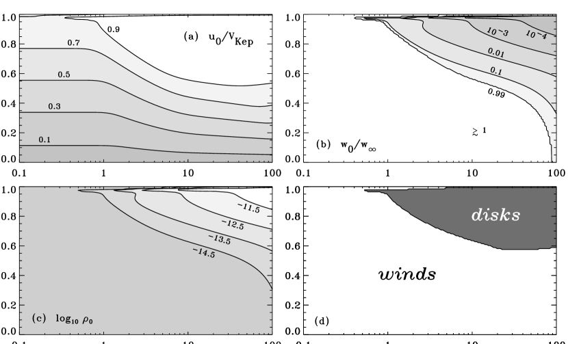
Figure 6.— Properties at the largest height ($z=80H_{0}$) for a grid of B2 V star models that vary $V_{\rm rot}$ and $V_{\rm puls}$ independently of one another: (a) ratio of rotation speed $u_{0}$ to Keplerian orbital speed $V_{\rm Kep}$, (b) ratio of radial wind speed $w_{0}$ to assumed terminal speed $w_{\infty}$, and (c) mean mass density $\rho_{0}$. Labels for constant contour values are given next to each curve. Panel (d) shows the heuristic dividing line between winds and disks (see text). See the last page of this paper for the full two-column version of this figure.

Figure 6c shows contours of the mean density $\rho_{0}$ at the top of the radial grid, which we take as a proxy for the density at the “inner edge” of the decretion disk. (For the models exhibiting Keplerian rotation, the density gradient is shallow and the plotted values of $\rho_{0}$ are insensitive to the exact height assumed for the upper edge of the grid.) The densities in Figure 6c range between a minimum of $3\times 10^{-16}$ g cm^-3 (lower left) and a maximum of $8\times 10^{-11}$ g cm^-3 (upper right), with the values exceeding $10^{-14}$ g cm^-3 tending to occur in the regime of parameter space filled by Keplerian disks. This range is consistent with observed inner disk densities. Traditional measurements from infrared excess (Waters et al.  1987) and visible linear polarization (McDavid 2001) give values between about $10^{-12}$ and $1.5\times 10^{-11}$ g cm^-3. More recent determinations that make use of H$\alpha$ profiles and interferometry (e.g., Gies et al.  2007; Jones et al.  2008) exhibit values that vary a bit more widely; essentially from $\sim$10^-13 to $10^{-9}$ g cm^-3. The latter end of this range, however, overlaps with estimated photospheric densities, and thus these values may be inconsistent with observational evidence that the photospheric layers rotate more slowly than $V_{\rm Kep}$.

Figure 6d illustrates the “bifurcation” of the models between winds and disks. For the purposes of this dividing line, a model is considered to have produced a Keplerian disk only if both $u_{0}/V_{\rm Kep}\geq 0.95$ and $w_{0}/w_{\infty}<0.1$. The latter condition ensures that an equatorial wind has not yet accelerated significantly by the top of the grid, which would invalidate the neglect of supersonic terms in equation (30).

Figure 7 shows a similar set of contours as Figure 6a, but the horizontal axis varies the reflection height $\Lambda$ as a free parameter (see § 3.2). The two-dimensional grid contained 120 values of $V_{\rm rot}/V_{\rm crit}$ distributed linearly between 0.01 and 0.995, and 200 values of $\Lambda/H_{0}$ distributed logarithmically between 1 and 500. This figure also includes the bifurcation curve as defined for Figure 6d. The photospheric NRP velocity amplitude was held fixed at 20 km s^-1. The combined effects of resonant excitation, shock dissipation, and wave pressure appear to produce roughly the same amount of angular momentum transport for $1\lesssim\Lambda/H_{0}\lesssim 20$. The “kink” in the contours at $\Lambda/H_{0}\approx 3.5$ corresponds to the reflection height at which the efficiency of resonant excitation saturates to unity somewhere above the photosphere (see Fig. 3). The largest values of the reflection height ($\Lambda/H_{0}\gtrsim 60$) do not give enough resonant excitation to produce substantial angular momentum transport in the upper atmosphere, so the contours approach the same kind of limiting shapes as are seen in Figure 6 for the limit $V_{\rm puls}\rightarrow 0$.

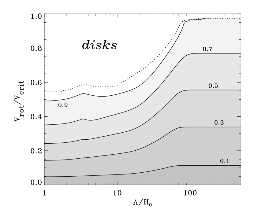
Figure 7.— Contours of $u_{0}/V_{\rm Kep}$ plotted similarly to Figure 6a, but for a grid of B2 V star models that vary $V_{\rm rot}$ and the reflection height $\Lambda$ independently of one another. The photospheric pulsation amplitude is held fixed at 20 km s^-1. The disk/wind boundary from Figure 6d is also shown (dotted line).

The final grid of models was produced by varying the rotation rate and the spectral type of the star, while keeping both $V_{\rm puls}$ and $\Lambda$ fixed at their standard values of 20 km s^-1 and $10H_{0}$, respectively. The grid contained 200 values of $V_{\rm rot}/V_{\rm crit}$ distributed linearly between 0.01 and 0.995, and 55 values of the spectral type in half-subtype increments between O3 and F0. Figure 8 shows contours of both $u_{0}/V_{\rm Kep}$ (Fig. 8a) and $w_{0}/w_{\infty}$ (Fig. 8b) along with the wind/disk bifurcation curve that is constrained by the combination of these two quantities. As before, the stellar parameters for each spectral type were taken from the $L_{\ast}$ and $T_{\rm eff}$ calibration of de Jager & Nieuwenhuijzen (1987), and $M_{\ast}$ was determined from the evolutionary tracks of Claret (2004). Fits for the mass-luminosity relations for luminosity classes III, IV, and V were given by Cranmer (2005). The models shown in Figure 8 follow the main sequence (i.e., luminosity class V).

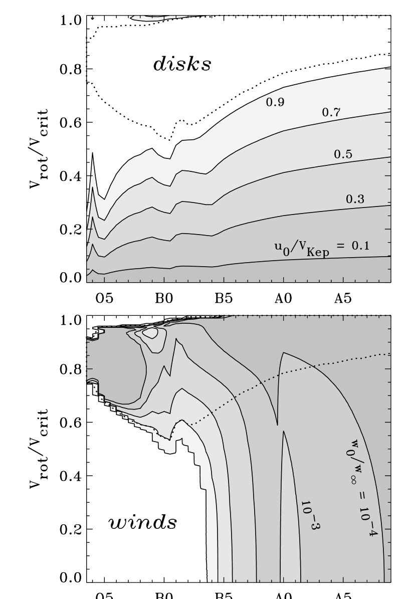
Figure 8.— Contours of $u_{0}/V_{\rm Kep}$ (top) and $w_{0}/w_{\infty}$ (bottom) plotted similarly to Figures 6a–b, but for a grid of main sequence models that vary $V_{\rm rot}$ and the spectral type independently of one another. The disk/wind boundary from Figures 6d and 7 is also shown in each panel (dotted lines).

The position of the dividing line between winds and disks depends (somewhat) on assumptions made about the equatorial mass loss rate and terminal speed. The fitting relations of Vink et al.  (2000) were used to estimate $\dot{M}$ as a function of the stellar parameters. The terminal speed was assumed to scale as $w_{\infty}=1.8V_{\rm esc}$, with the escape speed $V_{\rm esc}$ calculated at the pole (i.e., to estimate the polar wind’s terminal speed). The choice of the numerical constant 1.8 was motivated to reproduce the value of $w_{\infty}=1500$ km s^-1 used in the standard B2 V model discussed above. Although this constant has been seen to be as large as $\sim$3 for earlier O stars (Prinja et al.  1990), the shapes of the contours in Figure 8 were not seen to change when this constant was varied between 1.8 and 3.

Figure 8 pinpoints early B-type stars as those most likely to form Keplerian decretion disks with largest range of possible photospheric rotation rates. The O-type stars have stronger winds that require a more self-consistent (subsonic to supersonic) treatment of the radial momentum equation. Late B-type and all A-type stars appear to require only slightly larger rotation rates than early B stars to produce disks, but one should recall that the NRP amplitude was held fixed at 20 km s^-1 across these spectral types. In fact, most “normal” A stars (along and above the main sequence) are not as pulsationally unstable as the $\beta$ Cep and SPB stars, so their NRP amplitudes are likely to be significantly smaller than assumed here.

6. Discussion

6.1. Time Steady Disk Formation

How believable are the models presented above? This is a nontrivial question to ask when attempting to solve a problem that has plagued a discipline for three quarters of a century. The chain of events described in this paper remains somewhat speculative mainly because of the need to assume a finite reflection time (or reflection height $\Lambda$) that provides a time-steady yield of resonantly excited waves. If the resonant waves are much weaker than those predicted with $\Lambda\lesssim 20H_{0}$ (see Fig. 7), then this pulsational mechanism may not work. Additionally, if the frequency of resonant oscillations varies with height to stay equal to the local acoustic cutoff frequency (rather than remain at the piston’s cutoff frequency), then the waves may not propagate upward. In that case, the phase shift factors $\Phi_{1}$ and $\Phi_{2}$ (eq. [27]) could be much smaller than if the waves were propagating, and the ability to transport angular momentum would be reduced.

It is important to note, though, that there were several places in the above analysis where the wave coupling effects were decidedly underestimated. First, equation (11) neglects all higher-order transient terms (i.e., $t^{-5/2}$, $t^{-7/2}$, and so on) in the series expansion for the resonantly excited wave power. Second, equation (23) uses the local scale height $H(z)$ in the denominator of the wave pressure, rather than the smaller value at the piston that would have been more consistent with the use of a constant frequency $\omega$. Third, the Eulerian mass conservation equation (eq. [28]) was solved for $w_{0}$ instead of the Lagrangian version, resulting in a potentially weaker impact on the angular momentum transport. Fourth, this analysis totally neglected the fact that even purely evanescent waves can propagate energy in the horizontal direction (Walterscheid & Hecht 2003), and thus they may be able to exert a substantial wave pressure force in the azimuthal direction—even if they do not convert any of their energy into the resonant mode.

This paper made the implicit assumption that many early-type Be stars are rotating significantly below the critical limit, as suggested by, e.g., Slettebak (1982), Mennickent et al.  (1994), Porter (1996), and Cranmer (2005). If instead all Be stars are rotating close to critically (i.e., $V_{\rm rot}/V_{\rm crit}\gtrsim 0.95$) as suggested by Maeder & Meynet (2000) and Townsend et al.  (2004), the formation of disks could be accomplished with much more inefficient—and less speculative—physical mechanisms (see also Owocki 2005). In any case, for Be stars undergoing NRP with amplitudes of order the sound speed in their photospheres, many of the processes described in this paper should be occurring nevertheless.

6.2. Long-Term Be/Bn Phase Variability

The most prominent feature of Be stars that has not yet been addressed here is their substantial variability. Most noticeably, Be stars are known to exhibit phase changes between normal B (i.e., “Bn”), standard Be, and Be-shell properties (e.g., Slettebak 1988; Kogure 1990). These changes are typically interpreted as variations in the density and geometry of the circumstellar disk, though long-term changes in the properties of the photosphere have also been inferred (Doazan et al.  1986).

Although it was suggested earlier (§ 1) that a collection of other proposed mechanisms for producing Be-star disks may be responsible for some of the observed variability, it is worthwhile to also examine whether NRP/wave coupling would also contribute. In the models presented in this paper, the support of Be-star disks is provided ultimately by the kinetic and thermal energy in NRP motions. Thus, variations in the overall properties of the disk could be caused by variations of the stellar pulsations on the same kinds of time scales (i.e., long-term changes in the NRP “piston”). In fact, rapid stellar rotation has been shown to be connected with several kinds of pulsational variability and stochasticity:

1. The rotational splitting of NRP modes gives rise to closely separated periods that may be responsible for beating and amplitude modulations on time scales of weeks to months. For example, Rivinius et al.  (1998) found a set of periods for $\mu$ Cen that are separated by fractional frequency differences of order 0.01–0.02, such that the beating maxima and minima can occur with periods up to several years. There is also long-term drift in the precise values of many observed frequencies that could indicate beating or other kinds of multi-mode interactions (e.g., Štefl & Balona 1996; Sareyan et al.  1998). It has also been suggested (Henrichs 1984) that rotational splitting—especially for rapid rotation—may create additional “channels” of energy transfer between NRP and the mean state, and may even allow more pulsational energy to escape from the star.

2. As NRP modes grow to large amplitudes (i.e., $V_{\rm puls}\gtrsim c_{s}$) a host of nonlinear wave-wave interactions become possible that are not present in the linear, small-amplitude limit. There is observational evidence for a given NRP mode to grow slowly in amplitude, seemingly at the expense of another mode (Smith 1986). As a pulsation mode becomes nonlinear, it may even lose sinusoidal coherence by “interfering with itself” as it circumnavigates the star in longitude (e.g., Smith et al.  1987). If this occurs it could lead to shock steepening and dissipation in $\phi$, instead of in $r$ as assumed in § 3.3. The passage of an azimuthally propagating shock past a given point on the star could also act as a nonlinear trigger to restart the wave reflection “clock” for resonant excitation. Osaki (1999) suggested that a combination of these effects—along with feedback from the dense circumstellar envelope—would also lead to the eventual quenching of angular momentum transport, and thus to the dissipation of the disk. Such a repeated relaxation-oscillation cycle could be responsible for the phase variations between no disks (Bn), standard disks (Be), and optically thick disks (Be-shell).

3. The existence of subsurface convection could both impact the long-term growth or decay of pulsation modes and act as a seed for circumstellar variability (e.g., Cox 1980; Balmforth 1992; Gabriel 1998; Cantiello et al.  2009). Traditionally, B-type stars are not believed to have subsurface convection zones. There is some indirect evidence, however, that strong turbulent motions may be present near the surfaces of rapidly rotating early-type stars (Smith 1970; Kodaira 1980; Dolginov & Urpin 1983). Some recent models of oblate rapid rotators do show the emergence of a near-surface convection cell at the equator (Espinosa Lara & Rieutord 2007; Maeder et al.  2008). Even nonrotating hot stars—sufficiently above the main sequence—may exhibit enhanced subsurface convection due to newly discovered opacity peaks (Cantiello et al.  2009).

Although strictly unrelated to the stellar pulsations, another major source of long-term Be-star variability appears to be the naturally slow precession of non-axisymmetric density fluctuations through the dense Keplerian disk (e.g., Papaloizou et al.  1992; Savonije & Heemskerk 1993; Fiřt & Harmanec 2006). Gas parcels rotating under the influence of a non-point-mass gravitational potential undergo elliptical orbits with slow (decade timescale) pattern speeds. The modes that grow the fastest seem to be $m=1$, or “one-armed,” instabilities that appear to match the observed properties of the evolving violet-to-red ($V$/$R$) ratio of double-peaked Balmer emission line profiles. The ability to produce accurate and predictive models of these variations depends on understanding the origin and supply of angular momentum at the inner boundaries of the disks.

Finally, magnetic fields should not be neglected as an additional source of variability. Recent observational studies are beginning to reveal a distinct subclass of magnetic Be stars, which includes $\gamma$ Cas and at least a half-dozen others around spectral types B0e–B1e (Smith et al.  2004; Smith & Balona 2006; Rakowski et al.  2006; Lopes de Oliveira et al.  2007). Magnetic interactions between the star and the disk could be the source of dynamo action; i.e., another potential source of year- to decade-long variations in the circumstellar emission. Note that these processes may be acting whether or not the stellar wind is channeled along magnetic flux tubes to feed gas into the disk (e.g., Cassinelli et al.  2002; Brown et al.  2004, 2008; Ud-Doula et al.  2008).

7. Conclusions and Future Prospects

The primary aim of this paper has been to explore and test a set of physical processes that may be responsible for the production of Keplerian decretion disks around classical Be stars. Although nonradial pulsations correspond to low-frequency evanescent waves in the photospheres of hot stars, they have been suggested to give rise to higher frequency resonant oscillations at the acoustic cutoff frequency. If these resonant modes grow in amplitude with increasing height, begin to propagate upwards, and steepen into shocks, the resulting dissipation would create substantial wave pressure that both increases the atmospheric scale height and transports angular momentum upwards. Using a reasonable assumption for the efficiency of resonant wave generation, this chain of events was found to be able to create the inner boundary conditions required for a dense Keplerian disk, even when the underlying photosphere is rotating as slowly as $\sim$60% of its critical rotation speed.

It is important to note that in the models presented above, the “spinup” of the atmosphere occurs high enough above the photosphere so that standard measurements of the stellar rotation speed (i.e., $v\sin i$ from absorption line widths) would not be sensitive to these motions. The density at which the spinup is complete occurs several orders of magnitude below the photospheric ($\tau\approx 1$) density, and these values are consistent with inner-edge disk densities as measured by infrared excess and linear polarization techniques (see § 5.2). One way of potentially verifying that spinup is occurring in this thin layer would be to improve on measurements of spectral lines that are formed at a range of heights above the photosphere (see, e.g., Chen et al.  1989). In addition, the proposed scenario for resonant wave excitation implies that the dominant frequency of variability should shift from low (evanescent piston) to high (acoustic cutoff) values as the height increases.

In order to further test and verify that NRP-induced wave pressure is responsible for spinning up Be-star disk material, the physics of the resonant excitation process needs to be simulated more accurately. It may be possible to begin with one-dimensional simulations (similar to those of Fleck & Schmitz 1991) to explore both the time-steady yield of energy conversion from evanescent to resonant waves and the gradual increase in scale height due to radial wave pressure. Also, an analytic non-WKB treatment of partial wave reflection may shed light on how much intrinsic “leakage” the evanescent waves may undergo, even in the absence of resonant conversion (see Heinemann & Olbert 1980; Cranmer & van Ballegooijen 2005; Cranmer 2008).

Testing the full set of processes (e.g., resonant excitation, wave pressure, and angular momentum transfer) appears to require at least two-dimensional simulations of the fluid properties in the equatorial plane of a rotating hot star. These may take the form of next-generation extensions of studies by Kroll & Hanuschik (1997) and Owocki & Cranmer (2002), who showed that a large-amplitude NRP-like lower boundary could give rise to intermittent angular momentum transfer. Simulations may also benefit from an improved treatment of viscosity, which would be needed to extend the models upward to larger distances in the disk midplane (see, e.g., Lee et al.  1991; Okazaki 2001). It is likely that once simulations reveal the key physical processes, semi-analytic models like those presented in this paper can be improved to be more robust, predictively accurate, and less dependent on free parameters.

For the stellar models in which a supersonic wind begins to accelerate, a more physically realistic treatment of the radiative acceleration is needed. For example, the artificial imposition of a specific value for $\dot{M}$ should be replaced with a self-consistent calculation of the disk’s mass loss rate, which may be completely uncoupled from that of the polar wind. The proper modeling of B-type stellar outflows may also require an explicit treatment of collisional coupling between the various atomic and ionic species (Babel 1995; Krtička & Kubát 2001; Owocki & Puls 2002; Votruba et al.  2007) and a consistent solution for the internal energy equation, including both shock heating (e.g., Struck et al.  2004) and radiative scattering effects (Gayley & Owocki 1994).

Lastly, it should be emphasized that future work must involve not only increased physical realism for the models, but also quantitative comparisons with observations. It would be beneficial to apply the methodology outlined in this paper to a set of well-observed stars, rather than to the idealized spectral-type sequence illustrated in Figure 8. Measured stellar properties—including the dominant NRP velocity amplitudes—would be used as input constraints for models similar to those described in this paper. These models could then produce specific predictions for whether there should (or should not) be an equatorial disk for each star. Other models of the Be phenomenon, such as those summarized in § 1, will likely result in a different division of predicted disks versus non-disks for the same database of stars. Comparisons of each set of predictions with the observed occurrence of disks would act as a clear test of the viability of the proposed physical processes.

Appendix A Derivation of Second Order Wave Pressure Terms

For simplicity, the equations of hydrodynamic mass and momentum conservation are written below in Cartesian, plane-parallel coordinates. The vertical direction is $z$ and the relevant horizontal direction for oblique wave propagation is $x$. This geometry is applied to the equatorial plane of a rotating system, where $z$ points radially outward and $x$ points in the prograde azimuthal direction (i.e., increasing $x$ means increasing $\phi$ in the direction of rotational motion). We assume symmetry above and below the equatorial plane, so that all variations in colatitude $\theta$ (or Cartesian coordinate $y$) are ignored.

The two nontrivial velocity components are defined as $u=v_{x}$ and $w=v_{z}$. The equations of mass and momentum conservation are written as

$$\frac{\partial\rho}{\partial t}+\frac{\partial}{\partial x}(\rho u)+\frac{\partial}{\partial z}(\rho w)\,=\,0$$ (A1)

$$\frac{\partial}{\partial t}(\rho w)+\frac{\partial}{\partial x}(\rho uw)+\frac{\partial}{\partial z}(\rho w^{2})+\frac{\partial P}{\partial z}-\rho g\,=\,0$$ (A2)

$$\frac{\partial}{\partial t}(\rho u)+\frac{\partial}{\partial x}(\rho u^{2})+\frac{\partial}{\partial z}(\rho uw)+\frac{\partial P}{\partial x}\,=\,0\,\,.$$ (A3)

It is important to write the above equations in their full “conservation form.” Let us assume that all dynamical variables can be split into the sum of zeroth order (time steady) and first order (sinusoidally oscillating) components. Initially, the radial wind velocity $w_{0}(z)$ and the mean rotation velocity $u_{0}(z)$ are assumed to have arbitrary dependences on height. The mean density scale height is defined as $H\equiv-\rho_{0}/(\partial\rho_{0}/\partial z)$. All zeroth order properties are assumed to be constant in both time $t$ and horizontal position $x$.

Retaining only the zeroth order terms yields equations for the mean atmospheric stratification in the absence of wave pressure. Collecting the first order terms yields the dispersion relation as well as relative amplitude relations for linear waves. These are discussed by, e.g., Mihalas & Mihalas (1984) and Wang et al.  (1995), and the first-order expressions themselves are given in equations (7.82)–(7.90) of Cranmer (1996). The remainder of this Appendix deals with the second order terms; i.e., those that involve products of two first order fluid quantities. If the time average of a given second order term (taken over either a single wave period of an integer multiple of periods) does not vanish, then it gives rise to a net contribution to the time-steady conservation equations.

For example, the period-averaged mass flux conservation equation can be written as

$$\frac{\partial}{\partial z}(\rho_{0}w_{0})+\left\langle\frac{\partial}{\partial x}(\rho_{1}u_{1})\right\rangle+\left\langle\frac{\partial}{\partial z}(\rho_{1}w_{1})\right\rangle\,=\,0\,\,.$$ (A4)

The period-averaging is denoted by angle brackets. These terms can be simplified further by exploring some of the mathematical properties of such time averages. Consider a complex first order quantity $f=(f_{r}+if_{i})e^{i(\omega t-k_{x}x)}$, where the real amplitudes $f_{r}$ and $f_{i}$ are assumed to contain an unspecified dependence on $z$. For two such quantities ($f$ and $g$), the Eulerian average of their product over a period $2\pi/\omega$ has the following real part:

$$\langle fg\rangle\,=\,\frac{1}{2}(f_{r}g_{r}+f_{i}g_{i})\,=\,\frac{1}{4}(f^{\ast}g+fg^{\ast})$$ (A5)

where $f^{\ast}$ denotes the complex conjugate of $f$ and this averaged quantity is constant in $t$ and $x$. An additional and useful identity can be derived for these kinds of sinusoidal time variations,

$$\left\langle\frac{\partial}{\partial t}(fg)\right\rangle\,=\,\left\langle f\frac{\partial g}{\partial t}\right\rangle+\left\langle g\frac{\partial f}{\partial t}\right\rangle\,=\,0\,\,,$$ (A6)

and a similar identity can be defined by replacing $t$ with $x$, since the $x$ variations are ideally sinusoidal as well. (This cannot be done for the variations in $z$, however.) Thus, the second term in equation (A4) is zero, and the radial derivative in the third term can be taken outside the angle brackets to obtain

$$\frac{\partial}{\partial z}\left(\rho_{0}w_{0}+\langle\rho_{1}w_{1}\rangle\right)\,=\,0\,\,.$$ (A7)

This is the Lagrangian form of the mass conservation equation, which indicates that longitudinal and compressive waves can be responsible for a nonzero mass flux even in the absence of a mean local (Eulerian) flow velocity $w_{0}$. The ramifications of the $\langle\rho_{1}w_{1}\rangle$ term (also sometimes called the “Stokes drift”) are discussed in § 4.

The sum of the second order terms in the $x$ and $z$ components of the momentum conservation equation form a vector that we define as ${\bf S}=S_{x}\hat{\bf e}_{x}+S_{z}\hat{\bf e}_{z}$. Dimensionally, ${\bf S}$ has the units of a pressure gradient, or force per unit volume, and its components are

$$S_{x}\,=\,\frac{\partial}{\partial t}(\rho_{1}u_{1})+\frac{\partial}{\partial x}(\rho_{0}u_{1}^{2}+2\rho_{1}u_{0}u_{1})+\frac{\partial}{\partial z}(\rho_{0}u_{1}w_{1}+\rho_{1}u_{0}w_{1}+\rho_{1}u_{1}w_{0})$$ (A8)

$$S_{z}\,=\,\frac{\partial}{\partial t}(\rho_{1}w_{1})+\frac{\partial}{\partial x}(\rho_{0}u_{1}w_{1}+\rho_{1}u_{0}w_{1}+\rho_{1}u_{1}w_{0})+\frac{\partial}{\partial z}(\rho_{0}w_{1}^{2}+2\rho_{1}w_{0}w_{1})\,\,.$$ (A9)

These expressions can be simplified by noticing that the derivatives with respect to $t$ and $x$ can be neglected when constructing the period averages of $S_{x}$ and $S_{z}$. Thus, the mean azimuthal wave pressure gradient is given by

$$\langle S_{x}\rangle\,=\,\left\langle\frac{\partial}{\partial z}\left(\rho_{0}u_{1}w_{1}\right)\right\rangle+\left\langle\frac{\partial}{\partial z}\left(u_{0}\rho_{1}w_{1}\right)\right\rangle+\left\langle\frac{\partial}{\partial z}\left(w_{0}\rho_{1}u_{1}\right)\right\rangle\,\,.$$ (A10)

The first and second terms in equation (A10) are referred to by Lee & Saio (1993) and Lee (2007) as occurring on transport time scales $\tau_{1}$ and $\tau_{2}$, respectively. The third term depends on the Eulerian mean velocity $w_{0}$ and is traditionally ignored in stellar interiors models (for which the only mean motions are meridional circulations with speeds many orders of magnitude smaller than the pulsation amplitudes). We also neglect the $w_{0}$ term here (see below), and the remaining terms can be written as

$$\langle S_{x}\rangle\,=\,\frac{\partial}{\partial z}\left(\rho_{0}\langle u_{1}w_{1}\rangle\right)+\frac{\partial}{\partial z}\left(u_{0}\langle\rho_{1}w_{1}\rangle\right)\,\,.$$ (A11)

Because the first term above depends on $u_{1}$, its overall sign thus depends on the sign of $k_{x}$ (see eq. [7]). The second term, though, has the same sign no matter whether the waves are prograde or retrograde. For this term, it is straightforward to see that when $\rho_{1}$ and $w_{1}$ are in phase with one another (e.g., for an upwardly propagating wave) and $u_{0}$ is positive (i.e., for bulk rotation in the $+x$ direction), it behaves similarly to the radial wave pressure. In other words, if the pressure-like quantity being differentiated with respect to $z$ decreases as one goes up in height, it will result in a positive force (i.e., an upward acceleration for $S_{z}$ and an acceleration in the prograde direction for $S_{x}$).

The vertical (radial) wave pressure gradient can be condensed down to only two terms, with

$$\langle S_{z}\rangle\,=\,\left\langle\frac{\partial}{\partial z}\left(\rho_{0}w_{1}^{2}\right)\right\rangle+2\left\langle\frac{\partial}{\partial z}\left(w_{0}\rho_{1}w_{1}\right)\right\rangle\,\,.$$ (A12)

As above, the term depending explicitly on $w_{0}$ will be neglected here. Thus, the single remaining term

$$\langle S_{z}\rangle\,=\,\frac{\partial}{\partial z}\left(\rho_{0}\langle w_{1}^{2}\rangle\right)$$ (A13)

is equivalent to the plane-parallel limit of the wave pressure gradient derived elsewhere (e.g., Jacques 1977; Koninx 1992) in the limit of $\gamma=1$ (isothermal fluctuations). Also, the above expression is equivalent to equation (22) as long as the waves are sinusoidal in shape ($s=2$).

It should be emphasized that the above form of the radial wave pressure (eq. [A13]) is the same as that derived by Jacques (1977) and others, despite the fact that they do not make the assumption that $w_{0}=0$. In fact, they apply equation (A13) directly to the problem of how waves can help accelerate supersonic winds. Thus, it is likely that taking the limit of $w_{0}\rightarrow 0$ in the above equations is equivalent to transforming into the local comoving frame of reference of the fluid. The proper Reynolds stresses in $S_{x}$ and $S_{z}$ are those that add momentum to the fluid in the comoving (Lagrangian) frame.

Figure 6.— Properties at the largest height ($z=80H_{0}$) for a grid of B2 V star models that vary $V_{\rm rot}$ and $V_{\rm puls}$ independently of one another: (a) ratio of rotation speed $u_{0}$ to Keplerian orbital speed $V_{\rm Kep}$, (b) ratio of radial wind speed $w_{0}$ to assumed terminal speed $w_{\infty}$, and (c) mean mass density $\rho_{0}$. Labels for constant contour values are given next to each curve. Panel (d) shows the heuristic dividing line between winds and disks (see text).

References

- (1) Aerts, C., & de Cat, P. 2003, Space Sci. Rev., 105, 453
- (2) Ando, H. 1982, A&A, 108, 7
- (3) Ando, H. 1983, PASJ, 35, 343
- (4) Ando, H. 1986, A&A, 163, 97
- (5) Ando, H. 1988, in IAU Colloq. 108, Lecture Notes in Phys., 305, Atmospheric Diagnostics of Stellar Evolution: Chemical Peculiarity, Mass Loss, and Explosion, ed. K. Nomoto (Berlin: Springer-Verlag), 154
- (6) Baade, D. 1982, A&A, 105, 65
- (7) Baade, D. 1985, A&A, 148, 59
- (8) Baade, D., & Balona, L. A. 1994, in IAU Symp. 162, Pulsation, Rotation, and Mass Loss in Early-Type Stars, ed. L. A. Balona, H. F. Henrichs, & J. M. Le Contel (Dordrecht: Kluwer), 311
- (9) Babel, J. 1995, A&A, 301, 823
- (10) Balmforth, N. J. 1992, MNRAS, 255, 603
- (11) Bjorkman, J. E. 2000, in IAU Colloq. 175, ASP Conf. Ser. 214, The Be Phenomenon in Early-type Stars, ed. M. A. Smith, H. F. Henrichs, & J. Fabregat (San Francisco: ASP), 435
- (12) Bjorkman, J. E., & Cassinelli, J. P. 1993, ApJ, 409, 429
- (13) Bretherton, F. P. 1969, J. Fluid Mech., 36, 785
- (14) Bretherton, F. P., & Garrett, C. J. R. 1968, Proc. Roy. Soc. A, 302, 529
- (15) Brown, J. C., Cassinelli, J. P., & Maheswaran, M. 2008, ApJ, 688, 1320
- (16) Brown, J. C., Telfer, D., Li, Q., Hanuschik, R., Cassinelli, J. P., & Kholtygin, A. 2004, MNRAS, 352, 1061
- (17) Cantiello, M., Langer, N., Brott, I., de Koter, A., Shore, S. N., Vink, J., Voegler, A., Lennon, D. J., & Yoon, S.-C. 2009, A&A, in press, arXiv:0903.2049
- (18) Carciofi, A. C., & Bjorkman, J. E. 2006, ApJ, 639, 1081
- (19) Carlsson, M., & Stein, R. F. 1992, ApJ, 397, L59
- (20) Carlsson, M., & Stein, R. F. 1997, ApJ, 481, 500
- (21) Cassinelli, J. P., Brown, J. C., Maheswaran, M., Miller, N. A., & Telfer, D. C. 2002, ApJ, 578, 951
- (22) Castor, J. I. 1986, PASP, 98, 52
- (23) Castor, J. I., Abbott, D. C., & Klein, R. I. 1975, ApJ, 195, 157 (CAK)
- (24) Chen, H., Ringuelet, A., Sahade, J., & Kondo, Y. 1989, ApJ, 347, 1082
- (25) Claret, A. 2004, A&A, 424, 919
- (26) Collins, G. W., II 1963, ApJ, 138, 1134
- (27) Cox, J. P. 1980, The Theory of Stellar Pulsation (Princeton, NJ: Princeton Univ. Press)
- (28) Cranmer, S. R. 1996, Ph.D. Dissertation, University of Delaware
- (29) Cranmer, S. R. 2004, in SOHO-15: Coronal Heating, ed. R. W. Walsh, J. Ireland, D. Danesy, & B. Fleck (Noordwijk, The Netherlands: ESA), ESA SP-575, 154
- (30) Cranmer, S. R. 2005, ApJ, 634, 585
- (31) Cranmer, S. R. 2008, in IAU Symp. 250, Massive Stars as Cosmic Engines, ed. F. Bresolin, P. Crowther, & J. Puls (Cambridge: Cambridge Univ. Press), 526
- (32) Cranmer, S. R., & van Ballegooijen, A. A. 2005, ApJS, 156, 265
- (33) Cranmer, S. R., van Ballegooijen, A. A., & Edgar, R. J. 2007, ApJS, 171, 520
- (34) Dachs, J. 1987, in IAU Colloq. 92, Physics of Be Stars, ed. A. Slettebak & T. P. Snow (Cambridge: Cambridge Univ. Press), 149
- (35) de Cat, P. 2002, in IAU Colloq. 185, ASP Conf. Ser. 259, Radial and Nonradial Pulsations as Probes of Stellar Physics, ed. C. Aerts, T. Bedding, & J. Christensen-Dalsgaard (San Francisco: ASP), 196
- (36) de Cat, P. 2003, Ap&SS, 284, 37
- (37) de Cat, P. 2007, Commun. Asteroseismology, 150, 167
- (38) de Jager, C., & Nieuwenhuijzen, H. 1987, A&A, 177, 217
- (39) Dewar, R. L. 1970, Phys. Fluids, 13, 2710
- (40) Doazan, V. 1982, in B Stars with and without Emission Lines, NASA SP-456, ed. A. Underhill & V. Doazan, 277
- (41) Doazan, V., Thomas, R. N., & Barylak, M. 1986, A&A, 159, 75
- (42) Dolginov, A. Z., & Urpin, V. A. 1983, Ap&SS, 95, 1
- (43) Drew, J. E. 1989, ApJS, 71, 267
- (44) Dziembowski, W. A., & Pamyatnykh, A. A. 2008, MNRAS, 385, 2061
- (45) Eliassen, A., & Palm, E. 1960, Geofys. Publ., 22, 1
- (46) Erdélyi, R., Malins, C., Tóth, G., & De Pontieu, B. 2007, A&A, 467, 1299
- (47) Espinosa Lara, F., & Rieutord, M. 2007, A&A, 470, 1013
- (48) Fiřt, R., & Harmanec, P. 2006, A&A, 447, 277
- (49) Fleck, B., & Schmitz, F. 1991, A&A, 250, 235
- (50) Fullerton, A. W., Gies, D. R., & Bolton, C. T. 1996, ApJS, 103, 475
- (51) Gabriel, M. 1998, in Structure and Dynamics of the Interior of the Sun and Sun-like Stars, SOHO-6/GONG-98 Workshop, ed. S. Korzennik & A. Wilson (Noordwijk, The Netherlands: ESA), ESA SP-418, 863
- (52) Gautschy, A. 1992, MNRAS, 256, 11P
- (53) Gayley, K. G., Ignace, R., & Owocki, S. P. 2001, ApJ, 558, 802
- (54) Gayley, K. G., & Owocki, S. P. 1994, ApJ, 434, 684
- (55) Gies, D. R., et al. 2007, ApJ, 654, 527
- (56) Goldreich, P., & Nicholson, P. D. 1989, ApJ, 342, 1075
- (57) Grinin, V. P. 1978, Soviet Ast., 14, 301
- (58) Hanuschik, R. W. 1996, A&A, 308, 170
- (59) Heinemann, M., & Olbert, S. 1980, J. Geophys. Res., 85, 1311
- (60) Henrichs, H. F. 1984, in Fourth European IUE Conference, ed. E. Rolfe & B. Battrick (Noordwijk, The Netherlands: ESA), ESA SP-218, 43
- (61) Howarth, I. D., et al. 1993, ApJ, 417, 338
- (62) Howarth, I. D., Townsend, R. H. D., Clayton, M. J., Fullerton, A. W., Gies, D. R., Massa, D., Prinja, R. K., & Reid, A. H. N. 1998, MNRAS, 296, 949
- (63) Hummel, W., & Vrancken, M. 2000, A&A, 359, 1075
- (64) Jacques, S. A. 1977, ApJ, 215, 942
- (65) Jones, C. E., Tycner, C., Sigut, T. A. A., Benson, J. A., & Hutter, D. J. 2008, ApJ, 687, 598
- (66) Kalkofen, W., Rossi, P., Bodo, G., & Massaglia, S. 1994, A&A, 284, 976
- (67) Kambe, E., Ando, H., & Hirata, R. 1993a, A&A, 273, 435
- (68) Kambe, E., Ando, H., Hirata, R., Walker, G. A. H., Kennelly, E. J., & Matthews, J. M. 1993b, PASP, 105, 1222
- (69) Kaper, L., Henrichs, H. F., Nichols, J. S., Snoek, L. C., Volten, H., & Zwarthoed, G. A. A. 1996, A&AS, 116, 257
- (70) Kaufer, A., Stahl, O., & Prinja, R. K. 2007, in ASP Conf. Ser. 361, Active OB Stars: Laboratories for Stellar and Circumstellar Physics, ed. S. Štefl, S. P. Owocki, & A. T. Okazaki (San Francisco: ASP), 179
- (71) Kaufer, A., Stahl, O., Prinja, R. K., & Witherick, D. 2006, A&A, 447, 325
- (72) Kodaira, K. 1980, PASJ, 32, 435
- (73) Kogure, T. 1990, Ap&SS, 163, 7
- (74) Koninx, J. P. M. 1992, Ph.D. Dissertation, Rijksuniversiteit Utrecht
- (75) Kroll, P., & Hanuschik, R. W. 1997, in IAU Colloq. 163, ASP Conf. Ser. 121, Accretion Phenomena and Related Outflows, ed. D. T. Wickramasinghe, G. V. Bicknell, & L. Ferrario, 494
- (76) Krtička, J., & Kubát, J. 2001, A&A, 369, 222
- (77) Kubát, J. 2007, in ASP Conf. Ser. 361, Active OB Stars: Laboratories for Stellar and Circumstellar Physics, ed. S. Štefl, S. P. Owocki, & A. T. Okazaki (San Francisco: ASP), 281
- (78) Kurucz, R. L. 1992, in IAU Symp. 149, The Stellar Populations of Galaxies, ed. B. Barbuy & A. Renzini (Dordrecht: Kluwer), 225
- (79) Lamb, H. 1908, Proc. London Math. Soc., 7, 122
- (80) Lamb, H. 1932, Hydrodynamics (New York: Dover Publications)
- (81) Landau, L. D., & Lifshitz, E. M. 1959, Fluid Mechanics (Reading, Mass.: Addison-Wesley)
- (82) Lanz, T., & Hubeny, I. 2007, ApJS, 169, 83
- (83) Ledoux, P. 1951, ApJ, 114, 373
- (84) Lee, U. 2006, MNRAS, 365, 677
- (85) Lee, U. 2007, in ASP Conf. Ser. 361, Active OB Stars: Laboratories for Stellar and Circumstellar Physics, ed. S. Štefl, S. P. Owocki, & A. T. Okazaki (San Francisco: ASP), 45
- (86) Lee, U., Osaki, Y., & Saio, H. 1991, MNRAS, 250, 432
- (87) Lee, U. & Saio, H. 1993, MNRAS, 261, 415
- (88) Lopes de Oliveira, R., Motch, C., Smith, M. A., Negueruela, I., & Torrejón, J. M. 2007, A&A, 474, 983
- (89) Lou, Y.-Q. 1995, MNRAS, 276, 769
- (90) Maeder, A. 1999, A&A, 347, 185
- (91) Maeder, A., Georgy, C., & Meynet, G. 2008, A&A, 479, L37
- (92) Maeder, A., & Meynet, G. 2000, ARA&A, 38, 143
- (93) Massa, D. 1994, Ap&SS, 221, 113
- (94) Matthaeus, W. H., Zank, G. P., Oughton, S., Mullan, D. J., & Dmitruk, P. 1999, ApJ, 523, L93
- (95) McDavid, D. 2001, ApJ, 553, 1027
- (96) Mennickent, R. E., Vogt, N., Barrera, L. H., Covarrubias, R., & Ramírez, A. 1994, A&AS, 106, 427
- (97) Mihalas, D., & Mihalas, B. W. 1984, Foundations of Radiation Hydrodynamics (Oxford: Oxford U. Press)
- (98) Millar, C. E., & Marlborough, J. M. 1999, ApJ, 526, 400
- (99) Musielak, Z. E., Winget, D. E., & Montgomery, M. H. 2005, ApJ, 630, 506
- (100) Neilson, H. R., & Lester, J. B. 2008, ApJ, 684, 569
- (101) Okazaki, A. T. 2001, PASJ, 53, 119
- (102) Okazaki, A. T. 2007, in ASP Conf. Ser. 361, Active OB Stars: Laboratories for Stellar and Circumstellar Physics, ed. S. Štefl, S. P. Owocki, & A. T. Okazaki (San Francisco: ASP), 230
- (103) Osaki, Y. 1986, PASP, 98, 30
- (104) Osaki, Y. 1999, in IAU Colloq. 169, Variable and Non-Spherical Stellar Winds in Luminous Hot Stars, ed. B. Wolf, O. Stahl, & A. Fullerton (Berlin: Springer), 329
- (105) Owocki, S. P. 2005, in ASP Conf. Ser. 337, The Nature and Evolution of Disks around Hot Stars, ed. R. Ignace & K. G. Gayley (San Francisco: ASP), 101
- (106) Owocki, S. P., & Cranmer, S. R. 2002, in IAU Colloq. 185, ASP Conf. Ser. 259, Radial and Nonradial Pulsations as Probes of Stellar Physics, ed. C. Aerts, T. Bedding, & J. Christensen-Dalsgaard (San Francisco: ASP), 512
- (107) Owocki, S. P., Cranmer, S. R., & Gayley, K. G. 1996, ApJ, 472, L115
- (108) Owocki, S. P., & Puls, J. 2002, ApJ, 568, 965
- (109) Pantillon, F. P., Talon, S., & Charbonnel, C. 2007, A&A, 474, 155
- (110) Papaloizou, J. C., Savonije, G. J., & Henrichs, H. F. 1992, A&A, 265, L45
- (111) Pitteway, M. L. V., & Hines, C. O. 1965, Can. J. Phys., 43, 2222
- (112) Plumb, R. A. 1977, J. Atmos. Sci., 34, 1847
- (113) Poe, C. H., & Friend, D. B. 1986, ApJ, 311, 317
- (114) Porter, J. M. 1996, MNRAS, 280, L31
- (115) Porter, J. M., & Rivinius, T. 2003, PASP, 115, 1153
- (116) Prinja, R. 1989, MNRAS, 241, 721
- (117) Prinja, R., Barlow, M. J., & Howarth, I. D. 1990, ApJ, 361, 607
- (118) Rakowski, C. E., Schulz, N. S., Wolk, S. J., & Testa, P. 2006, ApJ, 649, L111
- (119) Rammacher, W., & Ulmschneider, P. 1992, A&A, 253, 586
- (120) Rivinius, T. 2007, in ASP Conf. Ser. 361, Active OB Stars: Laboratories for Stellar and Circumstellar Physics, ed. S. Štefl, S. P. Owocki, & A. T. Okazaki (San Francisco: ASP), 219
- (121) Rivinius, T., Baade, D., Štefl, S., Stahl, O., Wolf, B., & Kaufer, A. 1998, A&A, 336, 177
- (122) Rivinius, T., Baade, D., & Štefl, S. 2003, A&A, 411, 229
- (123) Rogers, T. M., MacGregor, K. B., & Glatzmaier, G. A. 2008, MNRAS, 387, 616
- (124) Rüdiger, G. 1977, Astron. Nachr., 298, 245
- (125) Saio, H. 1981, ApJ, 244, 299
- (126) Saio, H. 1994, in IAU Symp. 162, Pulsation, Rotation, and Mass Loss in Early-Type Stars, ed. L. A. Balona, H. F. Henrichs, & J. M. Le Contel (Dordrecht: Kluwer), 287
- (127) Sareyan, J. P., et al. 1998, A&A, 332, 155
- (128) Savonije, G. J., & Heemskerk, M. H. M. 1993, A&A, 276, 409
- (129) Schatzman, E. 1993, A&A, 279, 431
- (130) Schmidt, H. U., & Zirker, J. B. 1963, ApJ, 138, 1310
- (131) Schmitz, F., & Fleck, B. 1992, A&A, 260, 447
- (132) Slettebak, A. 1949, ApJ, 110, 498
- (133) Slettebak, A. 1982, ApJS, 50, 55
- (134) Slettebak, A. 1988, PASP, 100, 770
- (135) Smith, M. A. 1986, in Hydrodynamic and Magnetodynamic Problems in the Sun and Stars, ed. Y. Osaki (Tokyo: University of Tokyo), 145
- (136) Smith, M. A. 1988, in Pulsation and Mass Loss in Stars, Astrophys. Space Sci. Library v. 148, ed. R. Stalio & L. Willson (Dordrecht: Kluwer), 251
- (137) Smith, M. A., & Balona, L. 2006, ApJ, 640, 491
- (138) Smith, M. A., Cohen, D. H., Gu, M. F., Robinson, R. D., Evans, N. R., & Schran, P. G. 2004, ApJ, 600, 972
- (139) Smith, M. A., Fullerton, A. W., & Percy, J. R. 1987, ApJ, 320, 768
- (140) Smith, M. A., & Jeffery, C. S. 2003, MNRAS, 341, 1141
- (141) Smith, R. C. 1970, MNRAS, 148, 275
- (142) Štefl, S., Baade, D., Rivinius, T., Stahl, O., Budovičová, A., Kaufer, A., & Maintz, M. 2003, A&A, 411, 167
- (143) Štefl, S., & Balona, L. A. 1996, A&A, 309, 787
- (144) Sterken, C., & Jerzykiewicz, M. 1992, Space Sci. Rev., 62, 95
- (145) Struck, C., Smith, D. C., Willson, L. A., Turner, G., & Bowen, G. H. 2004, MNRAS, 353, 559
- (146) Struve, O. 1931, ApJ, 73, 94
- (147) Sutmann, G., Musielak, Z. E., & Ulmschneider, P. 1998, A&A, 340, 556
- (148) Talon, S. 2008, Mem. Soc. Astron. Italiana, 79, 569
- (149) Taroyan, Y., & Erdélyi, R. 2008, Sol. Phys., 251, 523
- (150) Telting, J. H. 2000, in IAU Colloq. 175, ASP Conf. Ser. 214, The Be Phenomenon in Early-type Stars, ed. M. A. Smith, H. F. Henrichs, & J. Fabregat (San Francisco: ASP), 422
- (151) Townsend, R. H. D. 2000a, in IAU Colloq. 175, ASP Conf. Ser. 214, The Be Phenomenon in Early-type Stars, ed. M. A. Smith, H. F. Henrichs, & J. Fabregat (San Francisco: ASP), 288
- (152) Townsend, R. H. D. 2000b, MNRAS, 318, 1
- (153) Townsend, R. H. D. 2000c, MNRAS, 319, 289
- (154) Townsend, R. H. D. 2005, MNRAS, 364, 573
- (155) Townsend, R. H. D. 2007, in AIP Conf. Proc. 948, Unsolved Problems in Stellar Physics, ed. R. Stancliffe, G. Houdek, R. Martin, & C. Tout (Melville, NY: AIP), 345
- (156) Townsend, R. H. D., & MacDonald, J. 2008, in IAU Symp. 250, Massive Stars as Cosmic Engines, ed. F. Bresolin, P. Crowther, & J. Puls (Cambridge: Cambridge Univ. Press), 161
- (157) Townsend, R. H. D., Owocki, S. P., & Howarth, I. D. 2004, MNRAS, 350, 189
- (158) Tubbesing, S., Rivinius, T., Wolf, B., & Kaufer, A. 2000, in IAU Colloq. 175, ASP Conf. Ser. 214, The Be Phenomenon in Early-type Stars, ed. M. A. Smith, H. F. Henrichs, & J. Fabregat (San Francisco: ASP), 232
- (159) Ud-Doula, A., Owocki, S. P., & Townsend, R. H. D. 2008, MNRAS, 385, 97
- (160) Vink, J. S., de Koter, A., Lamers, H. J. G. L. M. 2000, A&A, 362, 295
- (161) von Zeipel, H. 1924, MNRAS, 84, 665
- (162) Votruba, V., Feldmeier, A., Kubát, J., & Rätzel, D. 2007, A&A, 474, 549
- (163) Walterscheid, R. L., & Hecht, J. H. 2003, J. Geophys. Res., 108 (D11), 4340
- (164) Wang, Z., Ulrich, R. K., & Coroniti, F. V. 1995, ApJ, 444, 879
- (165) Waters, L. B. F. M., Coté, J., & Lamers, H. J. G. L. M. 1987, A&A, 185, 206
- (166) Willson, L. A. 1986, PASP, 98, 37
- (167) Willson, L. A. 2000, ARA&A, 38, 573
- (168) Woitke, P. 2007, in ASP Conf. Ser. 378, Why Galaxies Care About AGB Stars: Their Importance as Actors and Probes, ed. F. Kerschbaum, C. Charbonnel, R. Wing (San Francisco: ASP), 156
- (169) Yudin, R. V. 2001, A&A, 368, 912
- (170) Zahn, J.-P., Talon, S., & Matias, J. 1997, A&A, 322, 320