Shear rate threshold for the boundary slip in dense polymer films
Abstract
The shear rate dependence of the slip length in thin polymer films confined between atomically flat surfaces is investigated by molecular dynamics simulations. The polymer melt is described by the bead-spring model of linear flexible chains. We found that at low shear rates the velocity profiles acquire a pronounced curvature near the wall and the absolute value of the negative slip length is approximately equal to thickness of the viscous interfacial layer. At higher shear rates, the velocity profiles become linear and the slip length increases rapidly as a function of shear rate. The gradual transition from no-slip to steady-state slip flow is associated with faster relaxation of the polymer chains near the wall evaluated from decay of the time autocorrelation function of the first normal mode. We also show that at high melt densities the friction coefficient at the interface between the polymer melt and the solid wall follows power law decay as a function of the slip velocity. At large slip velocities the friction coefficient is determined by the product of the surface induced peak in the structure factor, temperature and the contact density of the first fluid layer near the solid wall.
pacs:
68.08.-p, 83.80.Sg, 83.50.Rp, 47.61.-k, 83.10.RsI Introduction
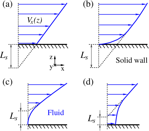
The rheology of complex fluids in thin films is important for theoretical and experimental studies of such common phenomena as friction, lubrication and wear Mate08 . Experimental measurements of the flow profiles and shear stresses on submicron scales might be subject to errors due to the possibility of liquid slip at the solid wall. An accurate prediction of flow, therefore, requires specification of a proper boundary condition. In the Navier model the interfacial shear rate and slip velocity are related via the proportionality coefficient, the so-called slip length. When the adjacent fluid layer slides past a solid wall with a finite velocity, the slip length is computed by linear extrapolation of the velocity profile near the interface to zero velocity [see Fig. 1 (a)]. In the case when there is no relative velocity between fluid and solid at the interface, the formation of a lower viscosity boundary layer might result in the apparent slip length which is defined by the slope of the bulk velocity profile VinogradLang95 [see Fig. 1 (b)]. Experimental studies on pressure-driven flows in microchannels or thin film drainage using either the surface force apparatus (SFA) or atomic force microscope (AFM) have demonstrated that the slip length depends on the nanoscale surface roughness Granick02 ; Archer03 ; Leger06 ; Vinograd06 , surface wettability Churaev84 ; Charlaix01 ; CottinEPJE02 , rate of shear Granick01 ; Granick02 ; CraigPRL01 ; GranLang02 ; Breuer03 ; Ulmanella08 , and fluid structure MackayVino ; SchmatkoPRL05 . Several slip regimes exist due to progressive disentanglement of the anchoring chains in the shear flow of polymer melts deGennes92 ; LegerPRL93 . The difficulty in experimental determination of the velocity profiles and structure of complex fluids near interfaces leaves open important questions regarding the shear rate dependency of the slip length and the existence of a shear rate threshold for the boundary slip.
In the last two decades, the boundary conditions at the interface between monatomic liquids and atomically flat walls were extensively studied by molecular dynamics (MD) simulations Fischer89 ; KB89 ; Thompson90 ; Barrat99 ; Barrat99fd ; Cieplak01 ; Quirke01 ; Attard04 ; Priezjev07 ; PriezjevJCP . The main factors affecting the slip are the energy of wall-fluid interaction and commensurability of the liquid and solid structures at the interface. At high wall-fluid energies, the first layer of fluid monomers becomes epitaxially locked to the solid substrate and the effective no-slip boundary plane is displaced into the fluid region. The absolute value of the negative slip length is approximately equal to the number of stacked monolayers between the effective and real boundary planes Fischer89 ; Thompson90 . At low surface energy, the first layer can slide with a finite velocity relative to the solid substrate under the shear stress from the bulk fluid [this situation is sometimes referred to as a molecular or ‘true’ slip, e.g., see Fig. 1 (a)]. The slip length is inversely proportional to the peak of the in-plane structure factor computed in the first fluid layer at the main reciprocal lattice vector Thompson90 ; Barrat99fd ; Priezjev07 . The exact relation between the slip length and microscopic parameters of the liquid/solid interface, however, has not yet been established.
The variation of the slip length with increasing shear rate in the flow of simple fluids past atomically smooth walls was first reported in the MD study by Thompson and Troian Nature97 . The nonlinear rate dependence of the slip length was well fitted by a power law function for different wall densities and weak wall-fluid interaction energies Nature97 . In a later study Priezjev07 , it was shown that the slip length is a linear function of shear rate at high wall-fluid interaction energies and, when the surface energy is reduced, the rate-dependence of the slip length can be well fitted by the power law function proposed in Ref. Nature97 . It was also found that in a wide range of shear rates and wall-fluid interaction energies, the slip length is a function of a single variable which combines temperature of the first fluid layer, the contact density, and the peak value of the in-plane fluid structure factor evaluated at the main reciprocal lattice vector Priezjev07 . The results of previous MD studies of monatomic fluids lead to a conclusion that the boundary conditions for flows past smooth surfaces are either no-slip and rate-independent Thompson90 or described by the finite positive slip length which increases with shear rate Nature97 ; Priezjev07 ; PriezjevJCP . Except for flows of low density fluids Fang05 , there was no reported observation of a transition from no-slip to steady-state slip flow with increasing shear rate for simple fluids.
The slip length in a flow of a polymer melt past a flat passive (non-adsorbing) surface is a ratio of the fluid viscosity to the friction coefficient which is determined by the interaction between fluid monomers and wall atoms deGennes85 . In a recent MD study of unentangled melts confined between smooth surfaces Priezjev04 , it was found that the friction coefficient at the liquid/solid interface is nearly independent of the chain length beyond ten bead-spring units and, therefore, the molecular weight dependence of the slip length at low shear rates is mostly dominated by the melt viscosity. Depending on the strength of the wall-fluid interaction energy, the slip occurs either at the confining surfaces Manias93 ; Thompson95 ; Manias96 ; dePablo96 ; StevensJCP97 ; Koike98 ; Tanner99 ; Priezjev04 ; Priezjev08 ; Servantie08 ; Pastorino08 ; Niavarani08 or between the adsorbed layer and free polymer chains Manias93 ; Manias96 . A transition from stick to slip flow with increasing shear rate was reported in MD simulations of thin films of hexadecane Tanner99 and oligomers Manias96 confined between strongly adsorbing surfaces. Despite extensive efforts in molecular simulations of thin polymer films, it still remains unclear what system parameters (fluid density, pressure, chain length, surface energy) determine the onset of boundary slip at the interface between an unentangled melt and a flat surface.
In a previous MD study Priezjev08 , the effect of shear rate on slip boundary conditions in thin polymer films confined between atomically smooth surfaces was investigated as a function of melt density. It was found that the slip length, extracted from the linear velocity profiles, passes through a local minimum at low shear rates and then increases rapidly at higher shear rates. This behavior was rationalized in terms of the friction coefficient (defined as a ratio of the shear-thinning viscosity to the slip length), which undergoes a gradual transition from a nearly constant value to the power law decay as a function of the slip velocity. The functional form of the relation between the friction coefficient and the slip velocity in the crossover region can also be considered as a boundary condition for monatomic fluids Priezjev08 ; Nature97 . In addition, it was shown that in a wide range of shear rates and melt densities, the friction coefficient is determined by the product of the value of surface induced peak in the structure factor, temperature and the contact density of the first fluid layer near the solid wall Priezjev08 . Whether these conclusions remain valid at higher melt densities (when a viscous interfacial layer is formed near the confined surfaces) is one of the motivations of the present study.
In this paper, we investigate the rate dependence of the slip length at the interface between an unentangled polymer melt and atomically flat walls using molecular dynamics simulations. We will show that in dense polymer films the velocity profiles are curved at low shear rates [shown schematically in Fig. 1 (c) and Fig. 1 (d)] due to highly viscous interfacial layer and the corresponding slip length is negative. When the viscosity of the interfacial layer is reduced at higher shear rates, the velocity profiles become linear and the slip length increases rapidly as a function of shear rate. The relaxation dynamics of polymer chains near the walls and in the bulk region is studied by analyzing the time autocorrelation function of the first normal mode at equilibrium and in shear flow. We will also show that the friction coefficient follows power law decay as a function of the slip velocity and its universal dependence on microscopic parameters of the liquid/solid interface holds only at large slip velocities.
The rest of this paper is organized as follows. The details of molecular dynamics simulations and the equilibration procedure are described in the next section. The fluid velocity and density profiles, shear rate dependence of the slip length, and the analysis of the fluid structure and relaxation dynamics of polymer chains are presented in Section III. The conclusions are given in the last section.
II Molecular dynamics simulation model
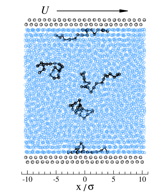
The simulation setup is similar to that described in the previous study Priezjev08 of a polymeric fluid undergoing planar shear flow between two atomically smooth walls. Figure 2 shows a snapshot of an unentangled polymer melt confined between solid walls. The total number of fluid monomers is kept the same as in the previous study () but the simulations are performed at higher fluid densities. The fluid monomers interact via the truncated Lennard-Jones (LJ) potential
| (1) |
where and are the energy and length scales of the fluid phase. The interaction between the wall atoms and fluid monomers is also modeled by the LJ potential with and . The wall atoms are tethered about the sites of an fcc lattice and do not interact with each other.
The coarse-grained bead-spring model was used to represent an unentangled polymer melt with linear chains of monomers. In addition to the LJ potential any two neighboring monomers in the chain interact through the finitely extensible nonlinear elastic (FENE) potential Bird87
| (2) |
with the standard parameters and Kremer90 . A combination of the LJ and FENE potentials between neighboring monomers yields an effective spring potential, which is strong enough to prevent polymer chains from unphysical crossing each other or bond breaking even at the highest shear rates considered in the present study.
The dynamics of fluid molecules and wall atoms was weakly coupled to a heat bath through a Langevin thermostat Grest86 . The thermostat was applied only to the component (perpendicular to the plane of shear) of the equations of motion for fluid monomers to avoid a bias in the shear flow direction Thompson90 . The equations of motion for fluid monomers in the , and directions are given by
| (3) | |||||
| (4) | |||||
| (5) |
where the sum is taken over the neighboring fluid monomers and wall atoms within the cutoff radius , is the friction coefficient, and is a random uncorrelated force with zero mean and variance determined from the fluctuation-dissipation relation. The temperature of the Langevin thermostat is set to , where is the Boltzmann constant. The equations of motion were integrated using the fifth-order gear-predictor algorithm Allen87 with a time step , where is the characteristic time of the LJ potential. The relatively small time step was chosen to resolve accurately the dynamics of fluid molecules and wall atoms at the interface.
The fluid is confined by the flat solid walls in the direction (see Fig. 2). Each wall consists of LJ atoms arranged in two layers of an fcc crystal with (111) plane parallel to the plane. The nearest-neighbor distance between fcc lattice sites in the plane is and the wall density is . The wall atoms were allowed to oscillate about their equilibrium lattice positions under the harmonic potential with the spring stiffness . The mean-square displacement of the wall atoms satisfies the Lindemann criterion for melting, i.e., . In addition, the random force and the damping term were applied to all three components of the wall atom equations of motion, e.g., for the component
| (6) |
where the mass of the wall atoms is , the friction coefficient is and the sum is taken over the fluid monomers within the cutoff distance . Periodic boundary conditions were applied in the and directions parallel to the walls.
The polymer melt was initially equilibrated for about at a constant normal pressure applied on the upper wall while the lower wall was kept at rest. Then, the external pressure was gradually increased to a desired value (reported in Table 1). The distance between the walls was fixed after the system was additionally equilibrated at the constant pressure for about . The MD simulations described below were performed at a constant density ensemble. The fluid density, the corresponding pressure in the absence of shear flow, and the channel height are listed in Table 1.
The shear flow was generated by moving the upper wall with a constant velocity in the direction parallel to the stationary lower wall. Before the production run started, the flow was simulated for about for each value of the upper wall speed. The fluid velocity and density profiles were averaged within bins of thickness for a time period up to at the lowest upper wall speed . The small bin size was chosen to resolve accurately the velocity profiles and fluid structure near the walls. At the highest shear rates examined in this study, the Reynolds number did not exceed the value estimated from the maximum difference of the fluid velocities near the upper and lower walls, the shear viscosity, the fluid density and the channel height (see Table 1).
III Results
III.1 Fluid density and velocity profiles
Molecular simulations of polymer melts confined by flat walls have demonstrated that the fluid structure consists of several discrete layers of monomers, the polymer chains are flattened near the walls, and the chain configurations remain bulklike in a region of several molecular diameters away from the walls Bitsanis90 . Qualitatively, these features can be observed in the snapshot of the polymer film shown in Fig. 2. Note that the first two layers of monomers near the walls are clearly distinguishable, the polymer chains in contact with the wall atoms are compressed towards the interface and their constitutive monomers are located within the discrete layers.
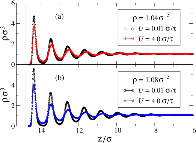
The representative density profiles are shown in Fig. 3 for and and two values of the upper wall speed. The density oscillations extend to a distance of about from the walls and the profiles are uniform in the central bulk region. The magnitude of the first peak near the wall defines a contact density . The amplitude of the density oscillations is reduced with increasing upper wall speed. Notice that at low in the case shown in Fig. 3 (b), the local density minimum between the first and second peaks is almost zero. It implies that the fluid monomers rarely jump between the first two layers, and it is, therefore, expected that the averaged velocity profiles will have relatively poor statistics in that region (see below).
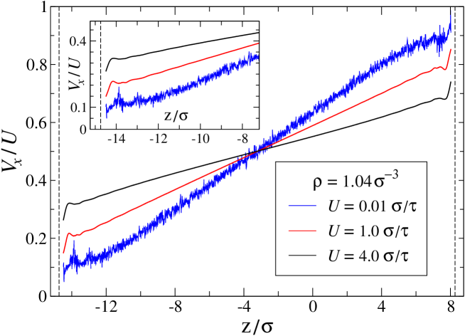
Figure 4 shows the averaged velocity profiles in steady-state flow for the lowest fluid density () considered in this study. The velocity profiles remain linear throughout the channel except for a larger slope inside the first fluid layer. A finite slip velocity is noticeable even at very low upper wall speed . The data are noisy because the averaged velocity component in the direction is much smaller than the thermal fluid velocity . The velocity profile for bends slightly near the walls, which implies that the interfacial viscosity is higher than the fluid bulk viscosity. A small curvature in the bulk region of the velocity profile at might be related to the nonuniform heating up of the fluid at high shear rates Priezjev08 . The normalized slip velocity increases with increasing upper wall speed.
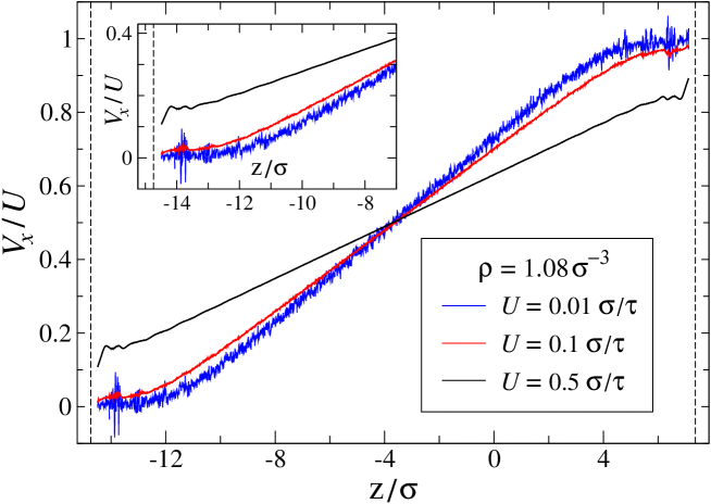
The averaged velocity profiles at the higher melt density () are reported in Fig. 5. At small values of the upper wall speed, the slip velocity of the first fluid layer is barely noticeable and the profiles are highly curved near the walls due to the presence of the viscous interfacial layer with thickness of about . The statistical fluctuations are relatively large near the walls because of the pronounced density layering [e.g., see Fig. 3 (b)]. The effective no-slip boundary plane is located inside the fluid domain at a distance of about from the wall. With increasing upper wall speed, the fluid velocity profiles become linear, the no-slip boundary plane is displaced out of the fluid region, and the slip velocity increases.
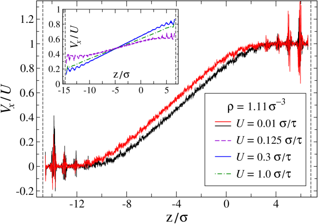
The normalized velocity profiles for the highest fluid density are plotted in Fig. 6. At the lowest upper wall speed , the first four monolayers stick to the walls but the velocity profiles remain linear in the middle of the channel. Due to the low probability of finding chain segments in between the monolayers the statistical uncertainties are much larger near the walls than in the bulk region. We found that the shape of the flow profiles depends on how the system was prepared. In one case, the upper wall speed was increased from zero to following the equilibration procedure described in the previous section. The averaged velocity profile is marked by the lower black curve in Fig. 6. In the other case, the upper wall speed was first increased to , and then, after the equilibration period of about , gradually reduced to . The corresponding velocity profile is shown by the upper red curve in Fig. 6. Note that the width of the flowing regions is nearly the same in both cases but the thickness of the immobile interfacial layers varies from about four to five molecular diameters. We also found that at higher upper wall speeds () the first fluid layer slides with a finite velocity past the substrate and the weak oscillations in the velocity profiles near the walls correlate with the fluid density layering (see inset in Fig. 6). Finally, as shown in the inset of Fig. 6, the velocity profiles become linear throughout the channel at higher upper wall speeds () and the slip velocity increases monotonically with increasing .
The slope of the linear part of the velocity profiles in the bulk region of the channel ( away from the walls) was used to compute the shear rate, shear stress and slip length. We define the slip length as a location of the point where linearly extrapolated velocity profile vanishes. Negative value of the slip length implies that the effective no-slip boundary plane is displaced into the bulk fluid domain. The velocity of the first fluid layer with respect to the lower stationary wall was computed as follows
| (7) |
where the limits of integration ( and ) were determined from the width of the first peak in the density profile. Note that even if the flow profiles are linear throughout the channel, the velocity of the first layer is slightly larger than the slip velocity computed from the Navier relation (by about in units of ). This is because the slip length is defined with respect to the reference plane away from the inner fcc lattice plane and the first fluid layer is located approximately away from the fcc plane (see Fig. 3).
III.2 Shear rate dependence of the melt viscosity and slip length
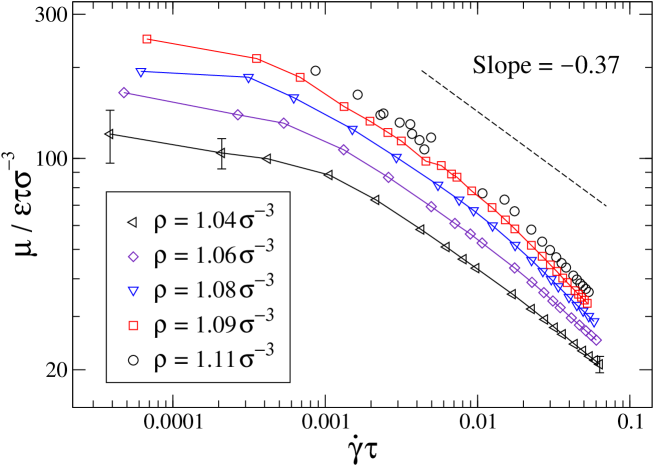
We first estimate the polymer melt viscosity which is defined as a ratio of shear stress to shear rate, i.e., . The shear stress was computed using the Kirkwood relation Kirkwood in the bulk region ( away from the confining walls), where the fluid structure is uniform and the velocity profiles are linear even at low shear rates. The viscosity is plotted in Fig. 7 as a function of shear rate for the indicated values of the polymer density. The Newtonian regime is observed only in a narrow range of shear rates, and it is followed by the crossover to the shear-thinning behavior, which occurs at higher shear rates when the melt density is reduced. The dashed line in Fig. 7 corresponds to the power law decay with the exponent reported for the lower density polymer melts () at high shear rates Priezjev08 . The data presented in Fig. 7 indicate that the melt viscosity in the shear-thinning regime decreases faster at higher fluid densities. The statistical errors due to thermal fluctuations are relatively large at low shear rates.
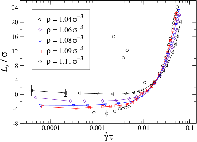
The variation of the slip length as a function of shear rate is presented in Fig. 8 for all melt densities considered. As expected from the shape of the velocity profiles described in the previous section, the slip length at low shear rates is negative (except for ) and its magnitude is approximately equal to the thickness of the viscous interfacial layer. With increasing shear rate, the velocity profiles become linear, implying that the local viscosity of the boundary layer is reduced, and the slip length increases rapidly. At the highest melt density and low shear rates, the thickness of the interfacial layer depends on the equilibration procedure and the slip length cannot be uniquely defined. The uncertainty in the slip length related to the thickness of the immobile interfacial layer and the slope of the velocity profile in the bulk region is about . At higher upper wall speeds () and , the first fluid layer is sliding with a finite velocity and the slip length is relatively large. Multivalued slip lengths were also reported in shear flow of simple fluids past smooth surfaces with high wall-fluid interaction energy Thompson90 . Finally, we comment that the data presented in Fig. 8 cannot be well fitted by the power law function proposed in Ref. Nature97 .
In our simulations, the upper wall speed was varied so that the slip velocity remains less than about the fluid thermal velocity. We performed test runs at higher upper wall speeds () and observed a different regime, where the the slip length becomes a nonmonotonic function of shear rate. It was also recently shown that the slip length at the interface between short chain polymers and smooth thermal walls approaches a constant value at high shear rates LichJFM08 ; LichPRL08 . In the present study, the behavior of the slip length at very large slip velocities and high shear rates was not examined in detail.
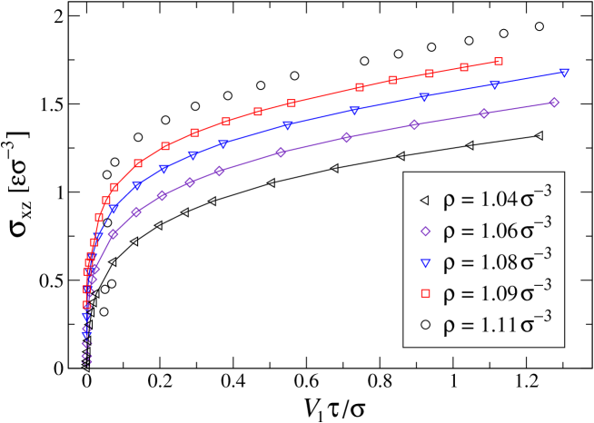
The rate-dependent boundary conditions can be reformulated in terms of the wall shear stress and slip velocity. In the steady-state shear flow, the stress across any plane parallel to the confining walls is the same, and, therefore, the shear stress computed in the bulk region is equal to the wall shear stress. The slip velocity of the first fluid layer was calculated by averaging the velocity profile over the width of the first density peak using Eq. (7). Note that the slip velocity computed from the Navier relation () is smaller than or can be even negative if the velocity profiles are curved near the interface [e.g., see Fig. 1 (c) and Fig. 1 (d)]. The shear stress averaged in the bulk region is plotted in Fig. 9 as a function of the slip velocity of the first fluid layer for the indicated polymer melt densities. The shear stress increases rapidly at small slip velocities and grows steadily at large . At the highest melt density , the time-averaged shear stress is discontinuous at small slip velocities.
The nonlinear relation between the shear stress and slip velocity shown in Fig. 9 can be used to determine the friction coefficient per unit area as a function of . We comment that the ratio of the shear viscosity to the slip length cannot be used to compute the friction coefficient at the liquid/solid interface when the velocity profiles are curved near the surface and the slip length is extracted from the bulk part of the profiles. In the previous study Priezjev08 , the simulations were performed at lower polymer melt densities and the velocity profiles remained linear at all shear rates examined. In the range of densities (), the friction coefficient () as a function of the slip velocity was well described by the following equation
| (8) |
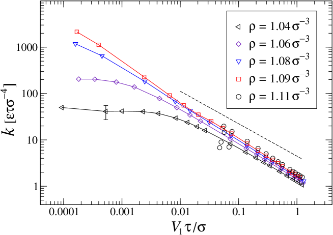
where and are the normalization parameters Priezjev08 . In the present study, the friction coefficient is plotted as a function of the slip velocity in Fig. 10. The data can be well fitted by the empirical formula Eq. (8) at lower melt densities (not shown). At higher melt densities , the plateau regime, where the friction coefficient is independent of the slip velocity, is absent and the slope of the power law decay is slightly smaller than (see the dashed line in Fig. 10).
III.3 Friction coefficient and fluid structure in the first layer
The connection between friction at the liquid/solid interface and fluid structure induced by the periodic surface potential was established for monatomic fluids Thompson90 ; Barrat99fd ; Priezjev05 ; Priezjev06 ; Priezjev07 ; PriezjevJCP , polymer melts Priezjev04 ; Priezjev08 , adsorbed monolayers Smith96 ; Tomassone97 and adsorbed polymer layers Muser06 . The in-plane structure factor in the first fluid layer near the solid substrate is defined as
| (9) |
where is the position vector of the -th monomer and is the number of monomers within the layer Thompson90 . Typically, the structure factor exhibits a circular ridge at the wavevector due to short range ordering of the fluid monomers. In addition, at sufficiently high wall-fluid interaction energy, several sharp peaks appear in the structure factor at the reciprocal lattice vectors of the crystal wall. It is well established that the magnitude of the peak at the first reciprocal lattice vector in the shear flow direction correlates well with the friction coefficient at the interface between a simple LJ liquid and a solid wall composed out of periodically arranged LJ atoms Thompson90 ; Barrat99fd ; Priezjev07 .
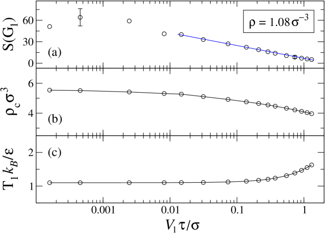
In the present study, the first reciprocal lattice vector in the shear flow direction is slightly displaced from the wavevector . The averaged structure factor is plotted in Fig. 11 (a) as a function of the slip velocity of the first fluid layer for the polymer density . The error bars are relatively large at small slip velocities due to the slow relaxation dynamics of the polymer chains in the interfacial layer (see next section). At higher slip velocities, fluid monomers spend less time in the minima of the periodic surface potential, and, as shown in Fig. 11 (a), the magnitude of the surface-induced peak in the structure factor decreases logarithmically with increasing . Furthermore, as expected from the density profiles shown in Fig. 3 for different upper wall speeds, the contact density is reduced at higher slip velocities [see Fig. 11 (b)]. Similarly to the definition of the slip velocity given by Eq. (7), the temperature of the first fluid layer was computed as follows
| (10) |
where is the local kinetic temperature and the limits of integration ( and ) were determined from the width of the first density peak. The variation of the monolayer temperature as a function of the slip velocity is presented in Fig. 11 (c). At small slip velocities , the temperature is equal to value set by the Langevin thermostat. With increasing upper wall speed, the temperature of the first fluid layer gradually rises up to at the highest slip velocity reported in Fig. 11 (c). At shear rates , the temperature profiles across the channel become nonuniform and the heating up is larger near the interfaces Priezjev08 .
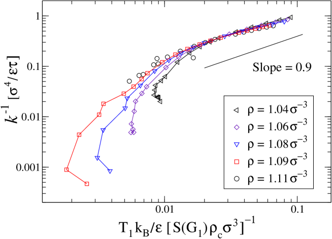
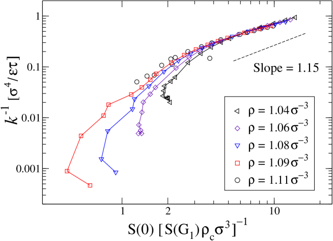
The dependence of the friction coefficient on the structure factor, contact density and temperature of the first fluid layer was studied in the recent paper Priezjev08 at lower polymer melt densities (). Except for the densities and at low shear rates, the data for the friction coefficient () were found to collapse on master curves when plotted as a function of either or . In both cases, the data could be well fitted by a power law function with the exponents and , respectively Priezjev08 . At higher polymer densities () considered in the present study, the inverse friction coefficient is plotted in Figures 12 and 13 as a function of the combined variables and , respectively. The collapse of the data holds at small values of the friction coefficient and the surface-induced peak in the structure factor . Thus, the simulations at higher melt densities provide an upper bound for the friction coefficient (), below which the data are described by a single master curve Priezjev08 . These results support the conclusion from the previous studies that at the interface between an atomically smooth solid wall and a simple Priezjev07 or polymeric Priezjev08 fluid, the friction coefficient is determined by a combination of parameters evaluated in the first fluid layer.
III.4 Relaxation dynamics of polymer chains
Equilibrium molecular dynamics studies of polymer melts confined between attractive walls have shown that the relaxation of polymer chains slows down near the interfaces and becomes bulk-like at distances of about two radiuses of gyration away from the walls Bitsanis93 ; Doi01 . In order to probe the relaxation dynamics of polymer chains in shear flow we evaluated the autocorrelation function of the normal modes in the direction perpendicular to the plane of shear. The component of the normal coordinates for a discrete polymer chain of monomers is given by
| (11) |
where is the component of the position vector of the -th monomer in the chain and is the mode number Binder95 . The longest relaxation time of a polymer chain is associated with the first mode . The normalized time autocorrelation function for the first normal mode is computed as follows
| (12) |
The relaxation dynamics in heterogeneous systems is usually described by the stretched exponential (or Kohlrausch-Williams-Watts) function . The time integral of the stretched exponential defines the characteristic decay time , where is the gamma function and is the stretched exponential coefficient.
The autocorrelation function, Eq. (12), was computed separately in the bulk region ( away from the solid walls) and inside the interfacial layers (within from the walls). During the simulation, the normal coordinate and the position of the center of mass of each polymer chain were calculated every , and the autocorrelation function was updated only if the position of the center of mass was inside either bulk or interfacial regions. The correlation function was averaged for at least at low shear rates to resolve very slow dynamics of the polymer chains near the interfaces.
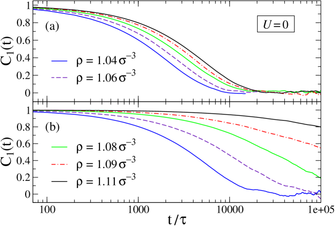
Figure 14 shows the time autocorrelation function computed at equilibrium conditions (i.e., ) for the indicated polymer densities. As expected, the relaxation of the polymer chains in the bulk and near the walls is slower at higher melt densities. The inverse bulk relaxation time, estimated roughly from in Fig. 14 (a), correlates well with the onset of shear thinning of the fluid viscosity reported in Fig. 7. For each density, the decay of the correlation function is slower for the chains in the interfacial layer than in the bulk of the channel. The difference in relaxation times is especially evident at higher melt densities, , where only the early stage of relaxation is reported in Fig. 14 (b). At the lowest polymer density , the decay time of the interfacial chains is about times larger than in the bulk, which agrees with the conclusion drawn from the shape of the velocity profile for in Fig. 4 that the interfacial viscosity is higher than the bulk value.
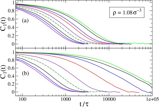
The influence of the shear flow on the time autocorrelation function is demonstrated in Fig. 15 for the polymer density . At low upper wall speeds , the relaxation dynamics near the interface is much slower than in the bulk region, implying the formation of a highly viscous interfacial layer. The spatial variation of the shear viscosity correlates with the nonlinearity in the velocity profiles shown in Fig. 5. When , the decay time of the correlation function is nearly the same across the channel (see the dashed curves in Fig. 15) and the velocity profile is linear (shown for in Fig. 5). At higher upper wall speeds, the polymer chains relax slightly faster near the walls than in the bulk, possibly because of the heating up of the fluid near the walls.
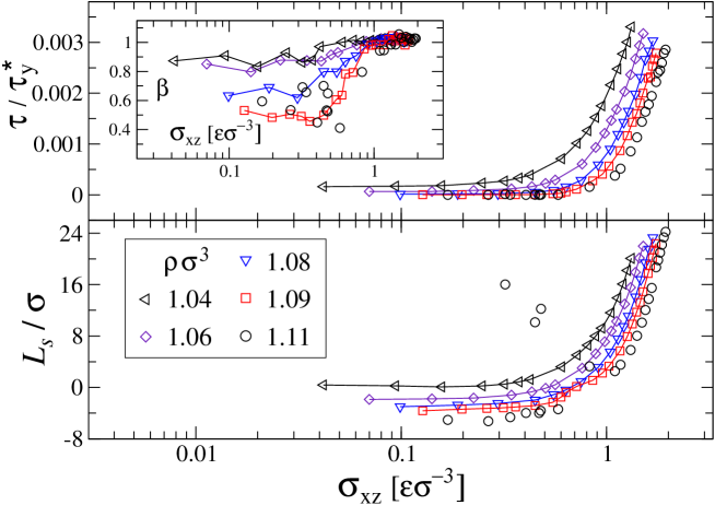
Finally, the relaxation time of the polymer chains near the walls and the slip length are summarized in Fig. 16 as a function of shear stress and polymer density. The leftmost points of the curves shown in Fig. 16 correspond to the upper wall speed . At low shear stress, the relaxation time varies widely from at to at , indicating the presence of a highly viscous boundary layer at higher melt densities. With increasing shear stress, the decay time decreases, and, when , the relaxation of the polymer chains near the walls becomes even slightly faster than in the bulk region (see also Fig. 15). The dependence the inverse relaxation time on the shear stress exhibits qualitatively similar behavior to the slip length, which supports the conclusion (drawn from the shape of the velocity profiles) that the transition to slip flow is associated with shear-melting of the boundary layer. The inset in Fig. 16 shows the variation of the stretched exponential coefficient as a function shear stress. The data are scattered at low shear stress due to the slow relaxation of the polymer chains, and the decay of the autocorrelation function becomes nearly exponential at higher shear stress.
IV Conclusions
In this paper, the rate-dependence of the slip length at the interface between a dense polymer melt and weakly attractive smooth walls was studied using molecular dynamics simulations. The melt was modeled as a collection of linear chain polymers (). It was shown that at low shear rates the velocity profiles are curved near the wall due to the formation of a highly viscous interfacial layer and the effective slip length is negative and almost rate-independent. With increasing upper wall speed, the gradual transition to steady-state slip flow is associated with shear-melting of the interfacial layer. The relaxation dynamics of polymer chains in shear flow was analyzed by evaluating the decay of time autocorrelation function of the first normal mode in the vorticity direction. We found that the rate behavior of the slip length correlates well with the inverse relaxation time of the polymer chains in the interfacial layer.
The rate-dependent slip boundary conditions were also reformulated in terms of the friction coefficient at the polymer/wall interface and slip velocity of the first fluid layer. In agreement with the results of the previous study Priezjev08 , we found that the friction coefficient at lower melt densities undergoes a transition from a constant value to the power law decay as a function of the slip velocity. At higher melt densities the friction coefficient decays as a power law function in a wide range of slip velocities. When the magnitude of the surface induced peak in the fluid structure factor is below a certain value, the friction coefficient is determined by a combination of parameters (structure factor, temperature, and contact density) of the first fluid layer near the solid wall.
Acknowledgments
Financial support from the Petroleum Research Fund of the American Chemical Society is gratefully acknowledged. Computational work in support of this research was performed at Michigan State University’s High Performance Computing Facility.
References
- (1) C. M. Mate, Tribology on the Small Scale: A Bottom Up Approach to Friction, Lubrication, and Wear (Oxford University Press, 2008).
- (2) O. I. Vinogradova, Langmuir 11, 2213 (1995).
- (3) Y. Zhu and S. Granick, Phys. Rev. Lett. 88, 106102 (2002).
- (4) J. Sanchez-Reyes and L. A. Archer, Langmuir 19, 3304 (2003).
- (5) T. Schmatko, H. Hervet, and L. Leger, Langmuir 22, 6843 (2006).
- (6) O. I. Vinogradova and G. E. Yakubov, Phys. Rev. E 73, 045302(R) (2006).
- (7) N. V. Churaev, V. D. Sobolev, and A. N. Somov, J. Colloid Interface Sci. 97, 574 (1984).
- (8) J. Baudry, E. Charlaix, A. Tonck, and D. Mazuyer, Langmuir 17, 5232 (2001).
- (9) C. Cottin-Bizonne, S. Jurine, J. Baudry, J. Crassous, F. Restagno, and E. Charlaix, Eur. Phys. J. E 9, 47 (2002).
- (10) Y. Zhu and S. Granick, Phys. Rev. Lett. 87, 096105 (2001).
- (11) V. S. J. Craig, C. Neto, and D. R. M. Williams, Phys. Rev. Lett. 87, 054504 (2001).
- (12) Y. Zhu and S. Granick, Langmuir 18, 10058 (2002).
- (13) C. H. Choi, K. J. A. Westin, and K. S. Breuer, Phys. Fluids 15, 2897 (2003).
- (14) U. Ulmanella and C.-M. Ho, Phys. Fluids 20, 101512 (2008).
- (15) R. G. Horn, O. I. Vinogradova, M. E. Mackay, and N. Phan-Thien, J. Chem. Phys. 112, 6424 (2000).
- (16) T. Schmatko, H. Hervet, and L. Leger, Phys. Rev. Lett. 94, 244501 (2005).
- (17) F. Brochard and P. G. de Gennes, Langmuir 8, 3033 (1992).
- (18) K. B. Migler, H. Hervet, and L. Leger, Phys. Rev. Lett. 70, 287 (1993).
- (19) U. Heinbuch and J. Fischer, Phys. Rev. A 40, 1144 (1989).
- (20) J. Koplik, J. R. Banavar, and J. F. Willemsen, Phys. Fluids A 1, 781 (1989).
- (21) P. A. Thompson and M. O. Robbins, Phys. Rev. A 41, 6830 (1990).
- (22) J.-L. Barrat and L. Bocquet, Phys. Rev. Lett. 82, 4671 (1999).
- (23) J.-L. Barrat and L. Bocquet, Faraday Discuss. 112, 119 (1999).
- (24) M. Cieplak, J. Koplik, and J. R. Banavar, Phys. Rev. Lett. 86, 803 (2001).
- (25) V. P. Sokhan, D. Nicholson, and N. Quirke, J. Chem. Phys. 115, 3878 (2001).
- (26) T. M. Galea and P. Attard, Langmuir 20, 3477 (2004).
- (27) N. V. Priezjev, Phys. Rev. E 75, 051605 (2007).
- (28) N. V. Priezjev, J. Chem. Phys. 127, 144708 (2007).
- (29) P. A. Thompson and S. M. Troian, Nature (London) 389, 360 (1997).
- (30) S. C. Yang and L. B. Fang, Molecular Simulation 31, 971 (2005).
- (31) P. G. de Gennes, Rev. Mod. Phys. 57, 827 (1985).
- (32) N. V. Priezjev and S. M. Troian, Phys. Rev. Lett. 92, 018302 (2004).
- (33) E. Manias, G. Hadziioannou, I. Bitsanis, and G. ten Brinke, Europhys. Lett. 24, 99 (1993).
- (34) P. A. Thompson, M. O. Robbins, and G. S. Grest, Israel Journal of Chemistry 35, 93 (1995).
- (35) E. Manias, G. Hadziioannou, and G. ten Brinke, Langmuir 12, 4587 (1996).
- (36) R. Khare, J. J. de Pablo, and A. Yethiraj, Macromolecules 29, 7910 (1996).
- (37) M. J. Stevens, M. Mondello, G. S. Grest, S. T. Cui, H. D. Cochran, and P. T. Cummings, J. Chem. Phys. 106, 7303 (1997).
- (38) A. Koike and M. Yoneya, J. Phys. Chem. B 102, 3669 (1998).
- (39) A. Jabbarzadeh, J. D. Atkinson, and R. I. Tanner, J. Chem. Phys. 110, 2612 (1999).
- (40) A. Niavarani and N. V. Priezjev, Phys. Rev. E 77, 041606 (2008).
- (41) J. Servantie and M. Muller, Phys. Rev. Lett. 101, 026101 (2008).
- (42) M. Muller, C. Pastorino, and J. Servantie, J. Phys. Condens. Matter 20, 494225 (2008).
- (43) A. Niavarani and N. V. Priezjev, J. Chem. Phys. 129, 144902 (2008).
- (44) R. B. Bird, C. F. Curtiss, R. C. Armstrong, and O. Hassager, Dynamics of Polymeric Liquids 2nd ed. (Wiley, New York, 1987).
- (45) K. Kremer and G. S. Grest, J. Chem. Phys. 92, 5057 (1990).
- (46) G. S. Grest and K. Kremer, Phys. Rev. A 33, 3628 (1986).
- (47) M. P. Allen and D. J. Tildesley, Computer Simulation of Liquids (Clarendon, Oxford, 1987).
- (48) I. Bitsanis and G. Hadziioannou, J. Chem. Phys. 92, 3827 (1990).
- (49) J. H. Irving and J. G. Kirkwood, J. Chem. Phys. 18, 817 (1950).
- (50) A. Martini, H. Y. Hsu, N. A. Patankar, and S. Lichter, Phys. Rev. Lett. 100, 206001 (2008).
- (51) A. Martini, A. Roxin, R. Q. Snurr, Q. Wang, and S. Lichter, J. Fluid Mech. 600, 257 (2008).
- (52) N. V. Priezjev, A. A. Darhuber, and S. M. Troian, Phys. Rev. E 71, 041608 (2005).
- (53) N. V. Priezjev and S. M. Troian, J. Fluid Mech. 554, 25 (2006).
- (54) E. D. Smith, M. O. Robbins, and M. Cieplak, Phys. Rev. B 54, 8252 (1996).
- (55) M. S. Tomassone, J. B. Sokoloff, A. Widom, J. Krim, Phys. Rev. Lett. 79, 4798 (1997).
- (56) D. Mukherji and M. H. Muser, Phys. Rev. E 74, 010601(R) (2006).
- (57) T. Aoyagi, J. Takimoto, and M. Doi, J. Chem. Phys. 115, 552 (2001).
- (58) I. A. Bitsanis and C. Pan, J. Chem. Phys. 99, 5520 (1993).
- (59) K. Binder, Monte Carlo and Molecular Dynamics Simulations in Polymer Science (Oxford University Press, 1995).