Nonlocal Form of the Rapid Pressure-Strain Correlation in Turbulent Flows

Abstract

A new fundamentally-based formulation of nonlocal effects in the rapid pressure-strain correlation in turbulent flows has been obtained. The resulting explicit form for the rapid pressure-strain correlation accounts for nonlocal effects produced by spatial variations in the mean-flow velocity gradients, and is derived through Taylor expansion of the mean velocity gradients appearing in the exact integral relation for the rapid pressure-strain correlation. The integrals in the resulting series expansion are solved for high- and low-Reynolds number forms of the longitudinal correlation function $f(r)$, and the resulting nonlocal rapid pressure-strain correlation is expressed as an infinite series in terms of Laplacians of the mean strain rate tensor. The new formulation is used to obtain a nonlocal transport equation for the turbulence anisotropy that is expected to provide improved predictions of the anisotropy in strongly inhomogeneous flows.

I Introduction

By far the most practical approaches for simulating turbulent flows are based on the ensemble-averaged Navier-Stokes equations. However, such approaches require a suitably accurate closure model for the Reynolds stress anisotropy tensor $a_{ij}$, defined as

$$a_{ij}\equiv\frac{\overline{u^{\prime}_{i}u^{\prime}_{j}}}{k}-\frac{2}{3}\delta_{ij}\,,$$ (1)

where $\overline{u^{\prime}_{i}u^{\prime}_{j}}$ are the Reynolds stresses and $k\equiv\frac{1}{2}\overline{u^{\prime}_{i}u^{\prime}_{i}}$ is the turbulence kinetic energy. Over the past half century, a wide range of closures for $a_{ij}$ have been proposed. Of these, so-called Reynolds stress transport models that solve the full set of coupled partial differential equations for $a_{ij}$ are currently regarded as having the highest fidelity among practical closures. Such closures start from the exact transport equation for $a_{ij}$, namely

$$\frac{Da_{ij}}{Dt}=-\left[\frac{P}{\epsilon}-1\right]\frac{\epsilon}{k}a_{ij}+\frac{1}{k}\left[P_{ij}-\frac{2}{3}P\delta_{ij}\right]+\frac{1}{k}\Pi_{ij}$$ (2)

$$-\frac{1}{k}\left[\epsilon_{ij}-\frac{2}{3}\epsilon\delta_{ij}\right]+\frac{1}{k}\left[D_{ij}-\left(a_{ij}+\frac{2}{3}\delta_{ij}\right)D\right]\,,$$

where for clarity we are restricting the presentation to incompressible flows. In (2), $D/Dt$ is the mean-flow material derivative, $P_{ij}\equiv-(\overline{u^{\prime}_{i}u^{\prime}_{l}}\ \partial\overline{u}_{j}/\partial x_{l}+\overline{u^{\prime}_{j}u^{\prime}_{l}}\ \partial\overline{u}_{i}/\partial x_{l})$ is the production tensor, $\epsilon_{ij}$ is the dissipation tensor, and all remaining viscous, turbulent, and pressure transport terms are contained in $D_{ij}$, with $P\equiv P_{nn}/2$, $\epsilon\equiv\epsilon_{nn}/2$, and $D\equiv D_{nn}/2$. In such Reynolds stress transport closures, the production tensor needs no modeling since $\overline{u^{\prime}_{i}u^{\prime}_{j}}$ is obtained from $a_{ij}$, and standard models for $\epsilon_{ij}$ and $D_{ij}$ are discussed in Refs. speziale1991 ; speziale1998 . The principal remaining difficulty is in accurately representing $\Pi_{ij}$ in (2), namely the pressure-strain correlation tensor

$$\Pi_{ij}(\textbf{x})\equiv\frac{2}{\rho}\,\overline{p^{\prime}(\textbf{x})S^{\prime}_{ij}(\textbf{x})}\,,$$ (3)

where

$$S^{\prime}_{ij}\equiv\frac{1}{2}\left(\frac{\partial u^{\prime}_{i}}{\partial x_{j}}+\frac{\partial u^{\prime}_{j}}{\partial x_{i}}\right)$$ (4)

are the strain rate fluctuations. The pressure-strain correlation has received considerable attention, however developing a fundamentally-based yet practically implementable form for $\Pi_{ij}$ remains one of the primary challenges in turbulence research.

The difficulty in representing $\Pi_{ij}$ stems in large part from the inherently nonlocal nature of the pressure-strain correlation, since the local pressure $p^{\prime}$ in (3) depends on an integral over the entire spatial domain of the flow. Some progress has been made by splitting $\Pi_{ij}$ into the sum of “slow” and “rapid” parts chou1945 , where the rapid part $\Pi^{(r)}_{ij}$ is so named due to its direct dependence on the mean-flow velocity gradients $\partial\overline{u}_{i}/\partial x_{j}$, variations in which have an immediate effect on $Da_{ij}/Dt$. Typically, the slow part $\Pi^{(s)}_{ij}$ is represented in terms of the local values of $a_{ij}$ and $\epsilon$. For the rapid part, it has been common (e.g., chou1945 ; rotta1951 ; crow1968 ) to take the mean velocity gradients as being sufficiently homogeneous that they can be brought outside the integral. Under certain conditions crow1968 the remaining integral can then be solved for the local part of $\Pi^{(r)}_{ij}$. This is then typically combined with additional ad hoc terms involving $a_{ij}$ to model the rapid part solely in terms of local flow variables. Together with the assumed local representation for the slow part, this yields a purely local formulation for $\Pi_{ij}$ that allows (2) to be solved, but that neglects all nonlocal effects in the evolution of the anisotropy.

Such purely local models for $\Pi_{ij}$ have allowed relatively accurate simulations of homogeneous turbulent flows, where by construction there are no spatial variations in $\partial\overline{u}_{i}/\partial x_{j}$ and thereby all nonlocal effects vanish. However most practical situations involve strongly inhomogeneous flows, where large-scale structure and other manifestations of spatial variations in the mean-flow velocity gradients can produce significant nonlocal effects in the turbulence, the neglect of which in $\Pi_{ij}$ can lead to substantial inaccuracies in the resulting anisotropy. Such nonlocal effects are significant even in free shear flows such as jets, wakes, and mixing layers, and can become especially important in near-wall flows, where flow properties vary rapidly in the wall-normal direction. Improving the fidelity of turbulent flow simulations requires a fundamentally-based formulation for nonlocal effects in $\Pi^{(r)}_{ij}$ to account for spatial variations of velocity gradients in the ensemble-averaged flow.

Various methods for addressing such spatial variations have been proposed, however nearly all suffer from a lack of systematic physical and mathematical justification. For near-wall flows, by far the most common yet also least satisfying approach is the use of empirical “wall damping functions” (e.g., speziale1998 ). Although such functions are relatively straightforward to implement, they are also distinctly ad hoc and as a consequence do not perform well across a wide range of flows. Moreover, wall functions typically conflate the treatment of a number of near-wall effects that in fact originate from distinctly different physical mechanisms, including low Reynolds number effects, large strain effects, and wall-induced kinematic effects, and are not formulated to specifically account for nonlocality due to spatial variations in the mean flow gradients.

In the following we depart from these prior approaches by systematically deriving a new nonlocal formulation for the rapid pressure-strain correlation from the exact integral relation for the rapid part of $\Pi_{ij}$. Specifically, nonlocal effects due to mean-flow velocity gradients are accounted for through Taylor expansion of $\partial\overline{u}_{k}/\partial x_{l}$ in the rapid pressure-strain integral. The resulting nonlocal form of the rapid pressure-strain correlation $\Pi^{(r)}_{ij}$ appears as a series of Laplacians of the mean strain rate tensor. The only approximation involved – beyond the central hypothesis on which the present formulation is based – is an explicit form for the longitudinal correlation function $f(r)$, though the effect of this is only to determine specific values of the coefficients in an otherwise fundamental result for the nonlocal effects in $\Pi^{(r)}_{ij}$. The coefficients are obtained here for the exponential form of $f(r)$ appropriate for high Reynolds numbers, and for the exact Gaussian $f(r)$ that applies at low Reynolds numbers. The resulting formulation for the rapid part of $\Pi_{ij}$ then provides a new nonlocal anisotropy transport equation that can be used with any number of closure approaches for representing $a_{ij}$, including Reynolds stress transport models as well as explicit stress models suitable for two-equation closures.

II Nonlocal Formulation for the Pressure-Strain Correlation

The starting point for developing a fundamentally-based representation for $\Pi_{ij}$ is the exact Poisson equation for the pressure fluctuations $p^{\prime}$ appearing in (3), namely

$$\frac{1}{\rho}\nabla^{2}p^{\prime}=-2\frac{\partial\overline{u}_{k}}{\partial x_{l}}\frac{\partial u^{\prime}_{l}}{\partial x_{k}}-\frac{\partial^{2}}{\partial x_{k}\partial x_{l}}\left(u^{\prime}_{k}u^{\prime}_{l}-\overline{u^{\prime}_{k}u^{\prime}_{l}}\right)\,$$ (5)

(e.g., pope2000 ). Beginning with Chou chou1945 , it has been common to write $p^{\prime}$ in terms of rapid, slow, and wall parts as

$$p^{\prime}\equiv p^{\prime(r)}+p^{\prime(s)}+p^{\prime(w)}\,,$$ (6)

defined by their respective Poisson equations from (5) as

$$\frac{1}{\rho}\nabla^{2}p^{\prime(r)}=-2\frac{\partial\overline{u}_{k}}{\partial x_{l}}\frac{\partial u^{\prime}_{l}}{\partial x_{k}}\,,$$ (7)

$$\frac{1}{\rho}\nabla^{2}p^{\prime(s)}=-\frac{\partial^{2}}{\partial x_{k}\partial x_{l}}\left(u^{\prime}_{k}u^{\prime}_{l}-\overline{u^{\prime}_{k}u^{\prime}_{l}}\right)\,,$$ (8)

$$\frac{1}{\rho}\nabla^{2}p^{\prime(w)}=0\,.$$ (9)

The effect of $p^{\prime(w)}$ is significant in (2) only in the extreme near-wall region of wall-bounded flows pope2000 ; mansour1988 . The remaining rapid and slow parts produce corresponding rapid and slow contributions to the pressure-strain correlation $\Pi_{ij}$ in (3), with Green’s function solutions of (7) and (8) giving these as

$$\Pi^{(r)}_{ij}(\textbf{x})=\frac{1}{\pi}\int_{\bf R}\frac{\partial\overline{u}_{k}(\hat{\textbf{x}})}{\partial\hat{x}_{l}}\overline{\frac{\partial u^{\prime}_{l}(\hat{\textbf{x}})}{\partial\hat{x}_{k}}S^{\prime}_{ij}(\textbf{x})}\frac{d^{3}\hat{\textbf{x}}}{|\textbf{x}-\hat{\textbf{x}}|}\,$$ (10)

$$\Pi^{(s)}_{ij}(\textbf{x})=\frac{1}{2\pi}\int_{\bf R}\overline{\frac{\partial^{2}\left(u^{\prime}_{k}u^{\prime}_{l}\right)_{\hat{\textbf{x}}}}{\partial\hat{x}_{k}\partial\hat{x}_{l}}S^{\prime}_{ij}(\textbf{x})}\frac{d^{3}\hat{\textbf{x}}}{|\textbf{x}-\hat{\textbf{x}}|}\,,$$ (11)

where the integration spans the entire flow domain R.

The slow part $\Pi^{(s)}_{ij}$ is typically not treated in a systematic fashion via integration of (11). Instead, nearly all existing representations for $\Pi_{ij}^{(s)}$ are based on insights obtained from the return to isotropy of various forms of initially-strained grid turbulence. The most common representation for $\Pi_{ij}^{(s)}$ is Rotta’s rotta1951 linear “return-to-isotropy” form

$$\Pi_{ij}^{(s)}=-C_{1}\epsilon a_{ij}\,,$$ (12)

where all variables are local and $C_{1}$ is typically in the range $1.5-1.8$ (e.g., speziale1998 ; pope2000 ). Sarkar and Speziale sarkar1990 ; speziale1991a have argued that additional quadratic terms should be included in (12), but it has been noted speziale1998 that these are typically small. As a result, representations for $\Pi_{ij}^{(s)}$ remain relatively simple, and the form in (12) continues to be widely used.

By contrast, $\Pi_{ij}^{(r)}$ has received substantially greater attention. The direct effect of the mean velocity gradients $\partial\overline{u}_{k}/\partial x_{l}$ on this rapid part of the pressure-strain correlation is apparent in (10). In the following sections, we use the integral in (10) to develop a fundamentally-based representation for $\Pi_{ij}^{(r)}$ that accounts for nonlocal effects resulting from spatial nonuniformities in the mean velocity gradients.

II.1 Prior Local Formulation for $\Pi_{ij}^{(r)}(\textbf{x})$

Chou chou1945 first suggested the notion of using the integral form in (10) to obtain a representation for the rapid pressure-strain correlation. Subsequently, Rotta rotta1951 and then Crow crow1968 used that approach to rigorously derive the purely local part of $\Pi_{ij}^{(r)}$, by assuming the mean velocity gradients in (10) to vary sufficiently slowly that they could be taken as constant over the length scale on which the two-point correlation $\overline{\left[\partial u^{\prime}_{k}(\hat{\textbf{x}})/\partial\hat{x}_{l}\right]S^{\prime}_{ij}(\textbf{x})}$ in (10) is nonzero. Under such conditions, the mean velocity gradient in (10) can be taken outside the integral, and $\Pi_{ij}^{(r)}$ then becomes

$$\Pi^{(r)}_{ij}(\textbf{x})\approx\frac{\partial\overline{u}_{k}(\textbf{x})}{\partial{x}_{l}}\cdot\frac{1}{\pi}\int_{\bf R}\overline{\frac{\partial u^{\prime}_{l}(\hat{\textbf{x}})}{\partial\hat{x}_{k}}S^{\prime}_{ij}(\textbf{x})}\frac{d^{3}\hat{\textbf{x}}}{|\textbf{x}-\hat{\textbf{x}}|}\,.$$ (13)

With $S^{\prime}_{ij}(\bf{x})$ in (3), the integrand in (13) involves two-point correlations among velocity gradients of the form

$$\overline{\frac{\partial u^{\prime}_{i}(\textbf{x})}{\partial x_{j}}\frac{\partial u^{\prime}_{l}(\hat{\textbf{x}})}{\partial\hat{x}_{k}}}=-\frac{\partial^{2}R_{il}(\textbf{r})}{\partial r_{j}\partial r_{k}}\,,$$ (14)

where $R_{il}(\textbf{r})$ denotes the velocity fluctuation correlation

$$R_{il}(\textbf{r})\equiv\overline{u^{\prime}_{i}(\textbf{x})u^{\prime}_{l}(\textbf{r}+\textbf{x})}$$ (15)

with $\textbf{r}\equiv\hat{\textbf{x}}-\textbf{x}$. Defining chou1945 ; rotta1951 ; crow1968

$$M_{iljk}\equiv-\frac{1}{2\pi}\int_{\bf R}\frac{\partial^{2}R_{il}(\textbf{r})}{\partial r_{j}\partial r_{k}}\frac{d^{3}\textbf{r}}{r}\,,$$ (16)

the rapid pressure-strain correlation in (13) can then be expressed as

$$\Pi_{ij}^{(r)}(\textbf{x})\approx\frac{\partial\overline{u}_{k}(\textbf{x})}{\partial x_{l}}\left[M_{iljk}+M_{jlik}\right]\,.$$ (17)

Using the homogeneous isotropic form of $R_{il}(\textbf{r})$, namely

$$R_{il}(r)=\frac{2}{3}k\left[f(r)\delta_{il}+\frac{r}{2}\frac{df}{dr}\left(\delta_{il}-\frac{r_{i}r_{l}}{r^{2}}\right)\right]\,$$ (18)

with

$$f(r)\equiv\frac{3}{2}\frac{\overline{u^{\prime}(\textbf{x}+\textbf{r})u^{\prime}(\textbf{x})}}{k}\,,$$ (19)

where $k$ is the turbulence kinetic energy, it can be shown crow1968 that $M_{iljk}$ in (16) becomes

$$M_{iljk}=\frac{2}{15}k\left(4\delta_{jk}\delta_{il}-\delta_{ij}\delta_{kl}-\delta_{jl}\delta_{ki}\right)\,,$$ (20)

where the leading $k$ again denotes the turbulence kinetic energy. Using (20) in (17) then gives the rapid pressure-strain correlation as

$$\frac{1}{k}\Pi_{ij}^{(r)}\approx\frac{4}{5}\overline{S}_{ij}\,,$$ (21)

where $\overline{S}_{ij}$ is the local mean-flow strain rate tensor

$$\overline{S}_{ij}\equiv\frac{1}{2}\left(\frac{\partial\overline{u}_{i}}{\partial x_{j}}+\frac{\partial\overline{u}_{j}}{\partial x_{i}}\right)\,.$$ (22)

Typically, (21) is used as the leading-order isotropic term in tensorial expansions for the rapid pressure-strain correlation $\Pi_{ij}^{(r)}(\textbf{x})$, where the remaining terms are expressed in terms of the local anisotropy $a_{ij}$ and the local mean velocity gradient tensor. Note however that such representations are still purely local, since in going from (10) to (13) all spatial variations in the mean velocity gradients $\partial\overline{u}_{k}/\partial x_{l}$ over the length scale on which the two-point correlations $\overline{\left[\partial u^{\prime}_{k}(\hat{\textbf{x}})/\partial\hat{x}_{l}\right]S^{\prime}_{ij}(\textbf{x})}$ are nonzero were ignored. The resulting neglect of nonlocal contributions to $\Pi^{(r)}_{ij}$ from that approximation can lead to substantial inaccuracies in many turbulent flows, including free shear flows and wall-bounded flows. For example, Bradshaw et al. bradshaw1987 showed using DNS of fully-developed turbulent channel flow kim1987 that the homogeneity approximation used to obtain (17) is invalid for $y^{+}\leq 30$. It can be further shown (e.g., kim1987 ; iwamoto2002 ) that the dominant component $\overline{S}_{12}$ of the mean strain begins to vary dramatically at locations as far from the wall as $y^{+}\approx 60$. Comparable variations in mean velocity gradients are also found in turbulent jets, wakes, and mixing layers, where there are substantial spatial variations in $\overline{S}_{12}$ across the flow. Indeed in most turbulent flows of practical interest, there are significant variations in the mean flow velocity gradients that will produce nonlocal contributions to the rapid pressure-strain correlation via (10). In such situations, it may be essential to account for these nonlocal effects in $\Pi_{ij}^{(r)}$ to obtain accurate results from any closures based on (2).

II.2 Present Nonlocal Formulation for $\Pi_{ij}^{(r)}(\textbf{x})$

In the following, nonlocal effects due to spatial variations in the mean flow are accounted for in $\Pi_{ij}^{(r)}$ through Taylor expansion of the mean velocity gradients appearing in (10). The central hypothesis in the approach developed here is that the nonlocality in $\Pi^{(r)}_{ij}$ is substantially due to spatial variations in $\partial\overline{u}_{k}/\partial x_{l}$ in (10), and that in order to address this effect all other factors in (10) can be adequately represented by their homogeneous isotropic forms. This allows a formulation of the rapid pressure-strain correlation analogous to that in (21), but goes beyond a purely local formulation to take into account the effects of spatial variations in the mean flow gradients.

We begin by defining the ensemble-averaged velocity gradients

$$A_{kl}\equiv\partial\overline{u}_{k}/\partial x_{l}\,,$$ (23)

and account for spatial variations in $A_{kl}(\hat{\textbf{x}})$ in (10) via its local Taylor expansion about the point x as

$$A_{kl}(\hat{\textbf{x}})=A_{kl}(\textbf{x})+r_{m}\frac{\partial A_{kl}}{\partial x_{m}}+\frac{r_{m}r_{p}}{2}\frac{\partial^{2}A_{kl}}{\partial x_{m}\partial x_{p}}$$ (24)

$$+\cdots+\frac{1}{n!}\left(r_{m}r_{p}\ldots\right)\frac{\partial^{n}A_{kl}}{\partial x_{m}\partial x_{p}\ldots}\,,$$

where $\textbf{r}\equiv\hat{\textbf{x}}-\textbf{x}$ and all derivatives of $A_{kl}$ are evaluated at x, and where $n$ is the order of the expansion. As $n\rightarrow\infty$, the expansion provides an exact representation of all spatial variations in $A_{kl}(\textbf{r}+\textbf{x})$ from purely local information at x. Substituting (24) into (10) then gives

$$\Pi_{ij}^{(r)}(\textbf{x})=\sum_{n=0}^{\infty}\frac{\partial^{n}A_{kl}(\textbf{x})}{\partial x_{m}\partial x_{p}\ldots}\left[{}_{(mp\ldots)}M^{(n)}_{iljk}+_{(mp\ldots)}M^{(n)}_{jlik}\right]\,,$$ (25)

where

$$_{(mp\ldots)}M^{(n)}_{iljk}\equiv-\frac{1}{2\pi n!}\int_{\bf R}\left[\frac{r_{m}r_{p}\ldots}{r^{n}}\right]r^{n-1}\frac{\partial^{2}R_{il}(\textbf{r})}{\partial r_{j}r_{k}}d^{3}\textbf{r}\,.$$ (26)

The $n$th-order term in (25) involves $n$ derivatives of $A_{kl}$ as well as $n$ total indices $(mp\ldots)$ in ${}_{(mp\ldots)}M^{(n)}_{iljk}$.

From the central hypothesis on which the present treatment of nonlocal effects in $\Pi^{(r)}_{ij}$ is based, we represent $R_{il}(\textbf{r})$ in (26) by the form in (18). With the relations

$$\frac{\partial r}{\partial r_{j}}=\frac{r_{j}}{r},\quad\frac{\partial r_{i}}{\partial r_{j}}=\delta_{ij}\,,$$ (27)

the double derivative of $R_{il}(\textbf{r})$ in (26) is then given by

$$\frac{\partial^{2}R_{il}(\textbf{r})}{\partial r_{j}\partial r_{k}}=\frac{k}{3}\left[a_{ijkl}\frac{1}{r}\frac{df}{dr}+b_{ijkl}\frac{d^{2}f}{dr^{2}}+c_{ijkl}r\frac{d^{3}f}{dr^{3}}\right]\,,$$ (28)

where we have introduced the compact notation

$$a_{ijkl}\equiv 3\delta_{jk}\delta_{il}-\delta_{ij}\delta_{kl}-\delta_{jl}\delta_{ki}-3\alpha_{jk}\delta_{il}+\delta_{ij}\alpha_{lk}$$ (29a)

$$+\delta_{jl}\alpha_{ik}+\delta_{ik}\alpha_{lj}+\delta_{kl}\alpha_{ij}+\delta_{kj}\alpha_{il}-3\beta_{iljk}\,,$$

$$b_{ijkl}\equiv\delta_{il}\delta_{jk}+3\alpha_{jk}\delta_{il}-\delta_{ij}\alpha_{lk}-\delta_{lj}\alpha_{ik}-\delta_{ik}\alpha_{lj}$$ (29b)

$$-\delta_{kl}\alpha_{ij}-\delta_{kj}\alpha_{il}+3\beta_{iljk}\,,$$

$$c_{ijkl}\equiv\delta_{il}\alpha_{jk}-\beta_{iljk}\,,$$ (29c)

with

$$\alpha_{ij}\equiv\frac{r_{i}r_{j}}{r^{2}}\,,\quad\beta_{ijkl}\equiv\frac{r_{i}r_{j}r_{k}r_{l}}{r^{4}}\,.$$ (30)

Writing the differential in (26) in spherical coordinates as $d^{3}\textbf{r}=r^{2}dr\ d\Omega$, where $d\Omega=\sin\theta\ d\theta\ d\phi$ and $r=[0,\infty)$, $\theta=[0,\pi]$, and $\phi=[0,2\pi)$, since $f(r)$ has no dependence on $\theta$ or $\phi$ and since $a_{ijkl}$, $b_{ijkl}$, and $c_{ijkl}$ in (29) have no dependence on $r$, the integrals over these terms in (26) can be considered separately. Using (28), the integral in (26) can then be written as

$${}_{(mp\ldots)}M^{(n)}_{iljk}=-\frac{k}{6\pi n!}\left[\int_{0}^{\infty}r^{n}\frac{df}{dr}dr\int_{\Omega}a_{ijkl}\frac{r_{m}r_{p}\ldots}{r^{n}}\ d\Omega\right.$$ (31)

$$+\int_{0}^{\infty}r^{n+1}\frac{d^{2}f}{dr^{2}}dr\int_{\Omega}b_{ijkl}\frac{r_{m}r_{p}\ldots}{r^{n}}\ d\Omega$$

$$\left.+\int_{0}^{\infty}r^{n+2}\frac{d^{3}f}{dr^{3}}dr\int_{\Omega}c_{ijkl}\frac{r_{m}r_{p}\ldots}{r^{n}}\ d\Omega\right]\,,$$

where $k$ in the leading factor is the turbulence kinetic energy. With the corresponding expression for ${}_{(mp\ldots)}M^{(n)}_{jlik}$, (25) and (31) provide a nonlocal form for the rapid pressure-strain rate correlation $\Pi^{(r)}_{ij}$ in terms of the longitudinal correlation $f(r)$.

II.3 Representing the Longitudinal Correlation $f(r)$

As will be seen later, in (31) the integrals over $d\Omega$ can be readily evaluated. Moreover, for $n=0$ the integrals over $dr$ are independent of $f(r)$, and thus $M^{(0)}_{iljk}$ can be obtained from the general properties

$$\Lambda=\int_{0}^{\infty}f(r)dr\,,\quad f(0)=1\,,\quad f(\infty)=0\,.$$ (32)

However for $n>0$, evaluating the integrals over $dr$ to obtain ${}_{(mp\ldots)}M^{(n)}_{jlik}$ requires an explicit form for the longitudinal correlation function $f(r)$. We can anticipate, however, that the precise form may not be of central importance to our eventual result for $\Pi^{(r)}_{ij}$, since the only role of $f(r)$ is to weight the contributions from velocity gradients $A_{kl}(\textbf{x}+\textbf{r})$ around the local point x. It is thus likely that the integral scale $\Lambda$ in (32) plays the most essential role, since it determines the size of the region around x from which nonlocal contributions to the integral for $\Pi^{(r)}_{ij}$ will be significant. When $r$ is scaled by $\Lambda$, the precise form of $f(r/\Lambda)$ is likely to be far less important for most reasonable forms that satisfy the constraints in (32).

Despite its fundamental significance in turbulence theory, the form of $f(r)$ for any $r$ and all Reynolds numbers $Re_{\Lambda}$ has yet to be determined even for homogeneous isotropic turbulence. Perhaps the most widely-accepted representation for $f(r)$ comes from Kolmogorov’s 1941 universal equilibrium hypotheses. For large values of $Re_{\Lambda}\equiv k^{1/2}\Lambda/\nu$ and inertial range separations $\lambda_{\nu}\ll r\ll\Lambda$, where $\lambda_{\nu}\sim(\nu^{3}/\epsilon)^{1/4}$ is the viscous diffusion scale and $\Lambda$ is the integral length scale in (32), the mean-square velocity difference is taken to depend solely on $r$ and the turbulent dissipation rate $\epsilon$, and thus on dimensional grounds must scale as

$$\overline{\left[u^{\prime}(\textbf{x}+\textbf{r})-u^{\prime}(\textbf{x})\right]^{2}}\sim\epsilon^{2/3}r^{2/3}\,.$$ (33)

Expanding the left-hand side of (33) and using (19) gives

$$\frac{4}{3}k\left[1-f(r)\right]\sim\epsilon^{2/3}r^{2/3}\,.$$ (34)

Defining the proportionality constant in (34) as $C_{f}$ and rearranging gives the inertial range form of $f(r)$ as

$$f(r)=1-\frac{3}{4}C_{f}\left[\frac{r}{k^{3/2}/\epsilon}\right]^{2/3}\,.$$ (35)

From Hinze hinze1975 , a value for $C_{f}$ can be obtained in terms of the Kolmogorov constant $K\equiv(8/9\alpha)^{2/3}\approx 1.7$, where $\alpha\approx 0.405$, as

$$C_{f}=\frac{81}{55}\,\,\Gamma(4/3)K\approx 2.24\,,$$ (36)

where we have used $\Gamma(4/3)\approx 0.893$. Expressing $\Lambda$ in terms of $k$ and $\epsilon$ on dimensional grounds as

$$\Lambda=C_{\lambda}\frac{k^{3/2}}{\epsilon}\,,$$ (37)

where $C_{\lambda}$ is a presumably universal constant, then allows the inertial-range form of $f(r)$ in (35) to be given as

$$f(r/\Lambda)=1-\frac{3}{4}C_{f}C_{\lambda}^{2/3}\left(\frac{r}{\Lambda}\right)^{2/3}\,.$$ (38)

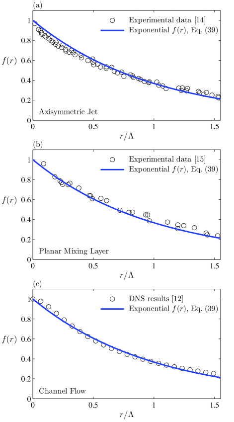
Figure 1: Comparison of exponential $f(r)$ in (39) with experimental data from axisymmetric turbulent jet wygnanski1969 (a) and planar turbulent mixing layer wygnanski1970 (b), and with DNS data from turbulent channel flow at $Re_{\tau}=650$ iwamoto2002 (c).

However the form for $f(r)$ in (38) is valid only for inertial-range $r$ values, namely $\lambda_{\nu}\ll r\ll\Lambda$ and thus for $Re_{\Lambda}^{-3/4}\ll(r/\Lambda)\ll 1$. As a consequence, this form cannot be used directly to evaluate the $r$-integrals in (31). However, experimental data from a wide range of turbulent free shear flows (e.g., wygnanski1969 ; wygnanski1970 ) and direct numerical simulation results for wall-bounded turbulent flows (e.g., kim1987 ; iwamoto2002 ) show that $f(r)$ can be reasonably represented by the exponential form

$$f(r/\Lambda)=e^{-r/\Lambda}\,,$$ (39)

as can be seen in Figures 1(a)-(c). Moreover, $C_{\lambda}$ in (37) can be chosen to closely match $f(r)$ in (39) with the fundamentally-rooted inertial-range form in (38). Indeed, Figure 2 shows that with

$$C_{\lambda}\approx 0.23$$ (40)

the exponential form in (39) gives reasonable agreement with the inertial-range form in (38) up to $r/\Lambda\approx 1$. This exponential form is thus here taken to represent $f(r)$ in high-$Re_{\Lambda}$ turbulent flows, and will be used in (31) to obtain an explicit form for the nonlocal rapid pressure-strain correlation. Since (25) with (31) is a rigorous formulation for $\Pi^{(r)}_{ij}$ within the central hypothesis on which the present approach is based, the exponential representation for $f(r)$ is the principal additional approximation that will be used below in deriving the present result for the rapid pressure-strain correlation.

While the exponential $f(r)$ appears appropriate for high $Re_{\Lambda}$, in the $Re_{\Lambda}\rightarrow 0$ limit the Kármán-Haworth equation karman1938 allows a solution for $f(r)$. Batchelor and Townsend batchelor1948 showed that when inertial effects can be neglected, this equation can be solved exactly, giving a Gaussian form for $f(r)$ as

$$f(r/\Lambda)=\exp\left[-\frac{4}{\pi}\left(\frac{r}{\Lambda}\right)^{2}\right]\,.$$ (41)

Ristorcelli ristorcelli1998 has proposed a blended form for $f(r)$ that satisfies various conditions placed on $f(r)$, including those in (32), while recovering the Gaussian $f(r)$ in (41) as $Re_{\Lambda}\rightarrow 0$ and the exponential $f(r)$ in (39) as $Re_{\Lambda}\rightarrow\infty$. It should be possible to use such blended forms for $f(r)$ to obtain a nonlocal pressure-strain correlation valid for all Reynolds numbers, following the procedure developed herein. In the following we obtain the nonlocal pressure-strain correlation using the high-Reynolds number exponential form in (39), which should be accurate for the vast majority of turbulent flow problems, and then show how this result can be extended to the low-Reynolds number limit using (41).

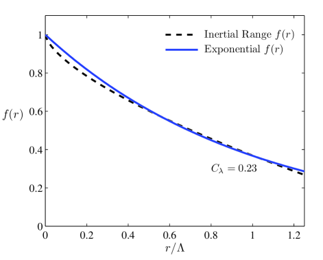
Figure 2: Comparison of inertial-range and exponential forms for $f(r/\Lambda)$ in (38) and (39), respectively. Note that $C_{\lambda}=0.23$ in (40) gives reasonable agreement between the two forms in the inertial range $Re_{\Lambda}^{-3/4}\ll(r/\Lambda)\ll 1$

II.4 Resulting Nonlocal Pressure-Strain Correlation

Using (39), it can be shown that the integrals over $dr$ in (31) give

$$\int_{0}^{\infty}r^{n}\frac{df}{dr}dr=-n!\Lambda^{n}\,,$$ (42a)

$$\int_{0}^{\infty}r^{n+1}\frac{d^{2}f}{dr^{2}}dr=(n+1)!\Lambda^{n}\,,$$ (42b)

$$\int_{0}^{\infty}r^{n+2}\frac{d^{3}f}{dr^{3}}dr=-(n+2)!\Lambda^{n}\,.$$ (42c)

With these results, (31) is then written as

$${}_{(mp\ldots)}M^{(n)}_{iljk}=k\frac{\Lambda^{n}}{6\pi}\int_{\Omega}\left[\frac{r_{m}r_{p}\ldots}{r^{n}}\right]\hskip 65.04256pt$$ (43)

$$\cdot\left[a_{ijkl}-(n+1)b_{ijkl}+(n+2)(n+1)c_{ijkl}\right]d\Omega\,.$$

The remaining integrals over $d\Omega$ are all of the form $(r_{m}r_{p}\ldots)/r^{n}$ and can be solved using the general integral relations

$$\int_{\Omega}\frac{r_{m}r_{p}r_{q}r_{s}\ldots}{r^{n}}d\Omega=0\,,\quad n=\textrm{odd}$$ (44a)

$$\int_{\Omega}\frac{r_{m}r_{p}r_{q}r_{s}\ldots}{r^{n}}d\Omega=\frac{4\pi}{(n+1)!!}\hskip 97.56493pt$$ (44b)

$$\cdot[\delta_{mp}\delta_{qs}\ldots+\delta_{mq}\delta_{rs}\ldots+\cdots]\,,\quad n=\textrm{even}$$

where the double factorial is defined as

$$n!!\equiv n(n-2)(n-4)\cdots\,,$$ (45)

with $0!!\equiv 1$ and $(-1)!!\equiv 1$, and the terms in brackets on the right-hand side of (44b) represent all possible combinations of delta functions for the indices $(m,p,q,s,\ldots)$. For any $n$, there are $(n-1)!!$ such delta function terms, and each term consists of $(n/2)$ delta functions.

In (43), for $n=0$ it can be shown using (44b) that $M^{(0)}_{iljk}$ is given by

$$M^{(0)}_{iljk}=k\frac{2}{15}\left(4\delta_{il}\delta_{jk}-\delta_{ij}\delta_{kl}-\delta_{jl}\delta_{ki}\right)\,.$$ (46)

For $n=1$, from (44a) ${}_{m}M^{(1)}_{iljk}=0$, as applies to all odd-$n$ cases. For $n=2$, from (44b) ${}_{mp}M^{(2)}_{iljk}$ is given by

$${}_{mp}M^{(2)}_{iljk}=\hskip 173.44756pt$$ (47)

$$k\frac{2\Lambda^{2}}{315}[4\delta_{jk}\delta_{il}\delta_{mp}-3\left(\delta_{ij}\delta_{kl}\delta_{mp}+\delta_{jl}\delta_{ik}\delta_{mp}\right)$$

$$-24\left(\delta_{il}\delta_{jm}\delta_{kp}+\delta_{il}\delta_{km}\delta_{jp}\right)+4(\delta_{ij}\delta_{lm}\delta_{kp}+\delta_{ij}\delta_{km}\delta_{lp}$$

$$+\delta_{jl}\delta_{im}\delta_{kp}+\delta_{jl}\delta_{km}\delta_{ip}+\delta_{ik}\delta_{lm}\delta_{jp}+\delta_{ik}\delta_{jm}\delta_{lp}$$

$$+\delta_{kl}\delta_{im}\delta_{jp}+\delta_{kl}\delta_{jm}\delta_{ip}+\delta_{jk}\delta_{im}\delta_{pl}+\delta_{jk}\delta_{lm}\delta_{ip})]\,.$$

Contracting (46) and (47) with $A_{kl}$ and its derivatives as in (25) then gives

$$A_{kl}\left[M^{(0)}_{iljk}+M^{(0)}_{jlik}\right]=\frac{4}{5}k\overline{S}_{ij}\,,$$ (48)

and

$$\frac{\partial^{2}A_{kl}}{\partial x_{m}\partial x_{p}}\left[{}_{mp}M^{(2)}_{iljk}+_{mp}M^{(2)}_{jlik}\right]=\frac{68}{315}k\Lambda^{2}\nabla^{2}\overline{S}_{ij}\,,$$ (49)

where we have used $A_{kk}\equiv 0$. From (48) and (49), the first two terms in the present formulation for the pressure-strain correlation in (25) are thus given by

$$\frac{1}{k}\Pi_{ij}^{(r)}(\textbf{x})=\frac{4}{5}\overline{S}_{ij}+\frac{68}{315}\Lambda^{2}\nabla^{2}\overline{S}_{ij}+\cdots\,.$$ (50)

The first term on the right in (50) is the same as that in (21) obtained by Crow crow1968 assuming spatially uniform mean velocity gradients. Thus the second term in (50) is the first-order nonlocal correction accounting for spatial variations in the mean velocity gradient field.

To obtain the remaining higher-order nonlocal corrections in (50), it is helpful to contract (43) with the derivatives of $A_{kl}$ and again use $A_{kk}\equiv 0$. It is then readily shown that all terms involving $\delta_{kl}$, $\delta_{km}$, $\delta_{kp}$, $\ldots$ from the integral over $d\Omega$ are zero when contracted with the derivatives of $A_{kl}$, and as a result the coefficients in (29) can be simplified as

$$a_{ijkl}=4\delta_{jk}\delta_{il}-\delta_{jl}\delta_{ki}-b_{ijkl}\,,$$ (51a)

$$b_{ijkl}=\delta_{il}\delta_{jk}+b^{*}_{ijkl}\,,$$ (51b)

$$b^{*}_{ijkl}=3\alpha_{jk}\delta_{il}-\delta_{lj}\alpha_{ik}-\delta_{ik}\alpha_{lj}-\delta_{kj}\alpha_{il}+3\beta_{iljk}\,,$$ (51c)

$$c_{ijkl}=\delta_{il}\alpha_{jk}-\beta_{iljk}\,,$$ (51d)

where $b^{*}_{ijkl}$ has been introduced to simplify the notation. Using (51) and contracting (43) with the derivatives of $A_{kl}$ we thus obtain

$$\frac{\partial^{n}A_{kl}}{\partial x_{m}\partial x_{p}\ldots}\left[{{}_{(mp\ldots)}}M^{(n)}_{iljk}\right]=\hskip 108.405pt$$ (52)

$$k\Lambda^{n}\frac{1}{6\pi}\left[\frac{\partial^{n}A_{kl}}{\partial x_{m}\partial x_{p}\ldots}\right]\int_{\Omega}\left[\frac{r_{m}r_{p}r_{q}\ldots}{r^{n}}\right]$$

$$\cdot[\left(2-n\right)\delta_{il}\delta_{jk}-\delta_{ik}\delta_{jl}-\left(n+2\right)b^{*}_{ijkl}$$

$$+(n+2)(n+1)c_{ijkl}]d\Omega\,.$$

From (44a) all odd-$n$ terms in (52) are zero. For even-$n$, the integrals over $d\Omega$ are readily evaluated using (44b), and it can then be shown that (52) becomes

$$\frac{\partial^{n}A_{kl}}{\partial x_{m}\partial x_{p}\ldots}\left[{{}_{(mp\ldots)}}M^{(n)}_{iljk}\right]=\hskip 108.405pt$$ (53)

$$k\Lambda^{n}\frac{2}{3}\left\{\frac{(n-1)!!}{(n+1)!!}\left(\nabla^{2}\right)^{n/2}\left[\left(2-n\right)A_{ji}-A_{ij}\right]\right.$$

$$-\frac{(n+2)(n-1)!!}{(n+3)!!}\left(\nabla^{2}\right)^{n/2}\left[(2-n)A_{ji}-A_{ij}\right]$$

$$+\frac{(n+2)(n+1)!!}{(n+3)!!}\left(\nabla^{2}\right)^{n/2}\left[A_{ji}+A_{ij}\right]$$

$$\left.-\frac{(n+2)(n+4)(n+1)!!}{(n+5)!!}\left(\nabla^{2}\right)^{n/2}\left[A_{ji}+A_{ij}\right]\right\}\,.$$

Adding the corresponding result for $M_{jlik}^{(n)}$ to (53) then gives $\Pi^{(r)}_{ij}$ from (25) as

$$\frac{1}{k}\Pi_{ij}^{(r)}=\sum_{n=0,even}^{\infty}\left[C_{2}^{(n)}\Lambda^{n}\left(\nabla^{2}\right)^{n/2}\overline{S}_{ij}\right]\,,$$ (54)

where the coefficients are

$$C_{2}^{(n)}\equiv\frac{4(n^{2}+2n+9)}{3(n+5)(n+3)(n+1)}\,.$$ (55)

Since the indices in (55) and (54) are required to be even, we can change the index $n$ to $(2n-2)$, where then $n=1,2,3,\ldots$. This gives the final result for the nonlocal rapid pressure-strain correlation from the present approach as

$$\frac{1}{k}\Pi_{ij}^{(r)}=C^{(1)}_{2}\overline{S}_{ij}+\sum_{n=2}^{\infty}\left[C_{2}^{(n)}\Lambda^{2n-2}\left(\nabla^{2}\right)^{n-1}\overline{S}_{ij}\right]\,$$ (56)

with

$$C_{2}^{(n)}\equiv\frac{16n^{2}-16n+36}{3(2n+3)(4n^{2}-1)}\,,$$ (57)

where $\Lambda$ in (56) is from (37) and (40). In (57) it may be readily verified that $C^{(1)}_{2}=4/5$ and $C^{(2)}_{2}=68/315$, consistent with (50) and (21). The first term on the right in (57) accounts for purely local effects on $\Pi^{(r)}_{ij}$, while the series term accounts for nonlocal effects.

The result in (56) and (57) is the first rigorous formulation for the rapid pressure-strain correlation $\Pi_{ij}^{(r)}$ that accounts for nonlocal effects due to spatial variations in the mean velocity gradients. Within the central hypothesis on which the present approach is based, the principal approximation used in deriving (56) and (57) is the exponential form of $f(r)$ in (39) for high-$Re_{\Lambda}$ turbulent flows. However, the only effect of this choice of $f(r)$ is in the resulting coefficients $C_{2}^{(n)}$ in (57). All other aspects of (56) are unaffected by the particular form of $f(r)$, and instead result directly from the fundamental approach taken here in solving (10) via Taylor expansion of the mean velocity gradients $\partial\overline{u}_{k}/\partial x_{l}$ to account for nonlocal effects in $\Pi_{ij}^{(r)}$.

The coefficients $C_{2}^{(n)}$ in (57) from the exponential representation of $f(r)$ are shown in Figure 3. It is apparent that the $n=1$ term in (56), which accounts for the purely local contribution to $\Pi_{ij}^{(r)}$ as verified in (50), is by far the dominant coefficient. The remaining coefficients for $n=2,3,4,\ldots$ correspond to the nonlocal contributions to $\Pi_{ij}^{(r)}$, and can be seen in Fig. 3 to decrease only slowly with increasing order $n$. However, while $C_{2}^{(1)}$ is clearly the dominant coefficient, in (56) the remaining coefficients are multiplied by successively higher-order Laplacians of the mean strain rate field, and thus may produce net contributions to $\Pi_{ij}^{(r)}$ that are comparable to, or possibly even larger than, the local term due to $n=1$.

II.5 Corresponding Coefficients for $Re_{\Lambda}\rightarrow 0$

While the coefficients in (57) are appropriate for $Re_{\Lambda}\gg 1$, in this Section we use the exact Gaussian form for $f(r)$ in (41) that applies in the $Re_{\Lambda}\rightarrow 0$ limit to obtain the result for $\Pi_{ij}^{(r)}$ applicable to low-$Re_{\Lambda}$ flows, as may occur in the near-wall region of wall-bounded turbulent flows. Using this form for $f(r)$, it can be shown that for even-$n$, which are the only nonzero terms from (43) due to (44a), the $r$-integrals in (31) are modified only by multiplying the previous results in (42) by the factor $\left[\left(2/\sqrt{\pi}\right)^{n}(n/2)!/n!\right]$. The result for $M^{(0)}_{iljk}$ in (46) is independent of the form of $f(r)$ and thus is unchanged in this limit, but now ${}_{mp}M^{(2)}_{iljk}$ in (47) is reduced by the factor $2/\pi$. With the remaining higher-order terms ${}_{(mp\ldots)}M^{(n)}_{iljk}$, it may be readily verified that the result for $\Pi_{ij}^{(r)}$ in (56) is unchanged in this low-$Re_{\Lambda}$ limit, but the coefficients $C_{2}^{(n)}$ are now given by

$$C_{2}^{(n)}=\frac{16n^{2}-16n+36}{3(2n+3)(4n^{2}-1)}\left[\frac{(n-1)!}{(2n-2)!}\left(\frac{4}{\pi}\right)^{n-1}\right]\,,$$ (58)

where again $n=1,2,3,\ldots$. The effect of the additional factor in (58) relative to (57) is to damp the higher-order terms in the $Re_{\Lambda}\gg 1$ coefficients, as shown in Fig. 3. It is apparent that in this $Re_{\Lambda}\rightarrow 0$ limit, only the first nonlocal term ($n=2$) in (56) is significant, with all higher-order coefficients being negligible. This may introduce significant simplifications in near-wall modeling, where this limit applies as $y^{+}\rightarrow 0$.

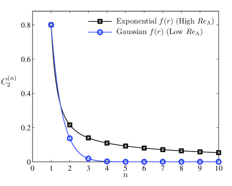
Figure 3: Comparison of rapid pressure-strain coefficients $C_{2}^{(n)}$ from (57) for the $Re_{\Lambda}\gg 1$ exponential $f(r)$ in (39), and from (58) for the $Re_{\Lambda}\rightarrow 0$ Gaussian $f(r)$ in (41).

II.6 Relation to Rotta rotta1951

The present result in (56) with (57) for $Re_{\Lambda}\gg 1$ or (58) for $Re_{\Lambda}\rightarrow 0$ is the first nonlocal pressure-strain correlation that rigorously accounts for the effect of spatial variations in the mean velocity gradients on the turbulence anisotropy. Previously, Rotta rotta1951 derived some of the components of $M^{(0)}_{iljk}$ and ${}_{mp}M^{(2)}_{iljk}$, though not enough to construct even the leading nonlocal term in (50). In particular, Rotta used an inertial-range form for $f(r)$ similar to (35) and the Gaussian form in (41) to obtain certain components of ${}_{mp}M^{(2)}_{iljk}$ in the high- and low-Reynolds number limits, respectively. Note that Rotta expressed his results rotta1951 in terms of the transverse integral scale $L$ rather than the longitudinal integral scale $\Lambda$. The two length scales are related by $L=0.5\Lambda$ for incompressible flows, and this relation can be used directly in the $Re_{\Lambda}\rightarrow 0$ limit to compare the present result for ${}_{mp}M^{(2)}_{iljk}$ with the components obtained by Rotta. For $Re_{\Lambda}\gg 1$, the differences between the inertial-range form of $f(r)$ used by Rotta and the exponential form in (39) used herein give his $L$ as $L=0.43\Lambda$. Using these relations it may be verified that the limited components of ${}_{mp}M^{(2)}_{iljk}$ given by Rotta are in agreement with the complete result in (47) for $Re_{\Lambda}\gg 1$, and with the result for $Re_{\Lambda}\rightarrow 0$ when the factor of $2/\pi$ is accounted for as noted in Section II.5.

The agreement with those components of ${}_{mp}M^{(2)}_{iljk}$ reported by Rotta rotta1951 provides partial validation of the present results. However, the present results go much further by addressing the complete components of ${}_{(mp\ldots)}M^{(n)}_{iljk}$ for all $n$, thereby allowing the first complete formulation of nonlocal effects in the rapid pressure-strain correlation $\Pi^{(r)}_{ij}$ due to spatial variations in the mean-flow gradients $\partial\overline{u}_{i}/\partial x_{j}$.

III Nonlocal Anisotropy Transport Equation

The present result for nonlocal effects in the rapid part $\Pi^{(r)}_{ij}$ of the pressure-strain correlation, given by (56) with the coefficients $C_{2}^{(n)}$ in (57) or (58) and with $\Lambda$ in (37) and (40), can be combined with (12) for the slow part $\Pi^{(s)}_{ij}$ to give $\Pi_{ij}$ in (2) as

$$\frac{1}{k}\Pi_{ij}=-C_{1}\frac{\epsilon}{k}a_{ij}+C^{(1)}_{2}\overline{S}_{ij}\hskip 108.405pt$$ (59)

$$+\sum_{n=2}^{\infty}\left[C^{(n)}_{2}\left(C_{\lambda}\frac{k^{3/2}}{\epsilon}\right)^{2n-2}\left(\nabla^{2}\right)^{n-1}\overline{S}_{ij}\right]\,.$$

In homogeneous flows, for which prior purely local models for $\Pi_{ij}$ have been relatively successful, the Laplacians of $\overline{S}_{ij}$ in (59) vanish, and thus the present nonlocal pressure-strain formulation recovers the local form in (21), since $C^{(1)}_{2}=4/5$ in both (57) and (58). For inhomogeneous flows, when (59) is introduced in (2) it gives a new anisotropy transport equation that accounts for both local and nonlocal effects via the present fundamental treatment of spatial variations in the mean velocity gradients in (10). Note in (2) that the definition of $P_{ij}$ with $P\equiv P_{nn}/2\equiv\overline{u^{\prime}_{i}u^{\prime}_{j}}\,\overline{S}_{ij}$ gives

$$\frac{1}{k}\left[P_{ij}-\frac{2}{3}P\delta_{ij}\right]\equiv-\frac{4}{3}\overline{S_{ij}}+\left(a_{il}\overline{W}_{lj}-\overline{W}_{il}a_{lj}\right)$$ (60)

$$-\left(a_{il}\overline{S}_{lj}+\overline{S}_{il}a_{lj}-\frac{2}{3}a_{nl}\overline{S}_{nl}\delta_{ij}\right)\,,$$

where the mean-flow rotation rate tensor $\overline{W}_{ij}$ is given by

$$\overline{W}_{ij}\equiv\frac{1}{2}\left(\frac{\partial\overline{u}_{i}}{\partial x_{j}}-\frac{\partial\overline{u}_{j}}{\partial x_{i}}\right)\,.$$ (61)

From (60), the production terms in (2) thus require no additional closure modeling, while current standard models summarized in Refs. speziale1991 ; speziale1998 may be used for the remaining $\epsilon_{ij}$ and $D_{ij}$ terms.

However, (59) does not account for possible additional anisotropic effects in $\Pi_{ij}^{(r)}$, since the present nonlocal pressure-strain result in (56) is based on the central hypothesis that $R_{il}(\textbf{r})$ in (26) can be represented by its isotropic form in (18). Fundamentally-based approaches for any such remaining anisotropic effects in (59) have yet to be rigorously formulated, however it has been heuristically argued ($e.g.$, launder1975 ; speziale1991a ) that such additional anisotropy effects may be represented by higher-order tensorial combinations of $a_{ij}$, $\overline{S}_{ij}$, and $\overline{W}_{ij}$. The most general of such combinations that remains linear in $a_{ij}$ is

$$\frac{1}{k}\Pi_{ij}^{(aniso)}=C_{3}\left(a_{il}\overline{S}_{lj}+\overline{S}_{il}a_{lj}-\frac{2}{3}a_{nl}\overline{S}_{nl}\delta_{ij}\right)$$ (62)

$$+C_{4}\left(a_{il}\overline{W}_{lj}-\overline{W}_{il}a_{lj}\right)\,,$$

where the constants $C_{3}$ and $C_{4}$ can be chosen to presumably account for such additional anisotropy effects. In general, choices for these coefficients vary widely from one model to another; a summary of various such models is given in Ref. speziale1998 .

When (59) is combined with (62), it provides an anisotropy transport equation that accounts for both local and nonlocal effects, as well as possible additional anisotropy effects, in the pressure-strain correlation as

$$\frac{Da_{ij}}{Dt}=-\alpha_{1}\frac{\epsilon}{k}a_{ij}+\alpha_{2}\overline{S}_{ij}\hskip 122.85876pt$$ (63)

$$+\sum_{n=2}^{\infty}\left[C^{(n)}_{2}\left(C_{\lambda}\frac{k^{3/2}}{\epsilon}\right)^{2n-2}\left(\nabla^{2}\right)^{n-1}\overline{S}_{ij}\right]$$

$$-\frac{1}{k}\left[\epsilon_{ij}-\frac{2}{3}\epsilon\delta_{ij}\right]+\alpha_{3}\left(a_{il}\overline{S}_{lj}+\overline{S}_{il}a_{lj}-\frac{2}{3}a_{nl}\overline{S}_{nl}\delta_{ij}\right)$$

$$-\alpha_{4}\left(a_{il}\overline{W}_{lj}-\overline{W}_{il}a_{lj}\right)+\frac{1}{k}\left[D_{ij}-\left(a_{ij}+\frac{2}{3}\delta_{ij}\right)D\right]\,,$$

where the $C_{2}^{(n)}$ coefficients are given in (57) or (58), and the $\alpha_{i}$ are defined as

$$\alpha_{1}=\frac{P}{\epsilon}-1+C_{1}\,,\quad\alpha_{2}=C_{2}^{(1)}-\frac{4}{3}\,,$$ (64)

$$\alpha_{3}=C_{3}-1\,,\quad\alpha_{4}=C_{4}-1\,.$$

Values for the constants $C_{1}$, $C_{3}$ and $C_{4}$ in (64) may be inferred from prior purely local models, such as the Launder, Reece and Rodi (LRR) launder1975 or Speziale, Sarkar and Gatski (SSG) speziale1991a models, which are all based on forms of (63) without the nonlocal effects given by the series term. However, optimal values for these constants may change in the presence of the nonlocal pressure-strain term in (64).

With respect to the remaining terms in (63), for high Reynolds numbers the dissipation tensor $\epsilon_{ij}$ is concentrated at the smallest scales of the flow, which are assumed to be isotropic. Thus, consistent with the central hypothesis on which the present result for the pressure-strain tensor is derived, the dissipation is commonly represented by its isotropic form $\epsilon_{ij}=\frac{2}{3}\epsilon\delta_{ij}$ (e.g., speziale1998 ; pope2000 ), with the result that the dissipation term in (63) vanishes entirely. The only remaining unclosed terms when (63) is used with the ensemble-averaged Navier-Stokes equations are the transport terms $D_{ij}$ and $D$, and these are typically represented using gradient-transport hypotheses, with several possible such formulations summarized in Ref. speziale1998 .

A number of different approaches can be taken for solving (63). First, this may be solved as a set of six coupled partial differential equations, together with the ensemble-averaged Navier-Stokes equations, to obtain a new nonlocal Reynolds stress transport closure that improves on existing approaches such as the LRR and SSG models in strongly inhomogeneous flows. Alternatively, equilibrium approximations may be used to neglect the $Da_{ij}/Dt$ and $D_{ij}$ terms in (63) to obtain a new explicit nonlocal equilibrium stress model for $a_{ij}$, analogous to the existing local models developed, for example, by Gatski and Speziale gatski1993 , Girimaji girimaji1996 , and Wallin and Johannson wallin2000 . Perhaps preferably, a new explicit nonlocal nonequilibrium stress model for $a_{ij}$ can be obtained from (63) following the approach in Ref. hamlington2008a , by explicitly solving the quasi-linear form of (63), namely

$$\frac{Da_{ij}}{Dt}=-\alpha_{1}\frac{\epsilon}{k}a_{ij}+\alpha_{2}\overline{S}_{ij}\hskip 122.85876pt$$ (65)

$$+\sum_{n=2}^{\infty}\left[C^{(n)}_{2}\left(C_{\lambda}\frac{k^{3/2}}{\epsilon}\right)^{2n-2}\left(\nabla^{2}\right)^{n-1}\overline{S}_{ij}\right]\,.$$

In so doing it is possible to obtain a new explicit form for the anisotropy $a_{ij}$ that accounts for both nonlocal and nonequilibrium effects in turbulent flows.

IV Conclusions

A new rigorous and complete formulation for the rapid pressure-strain correlation, including both local and nonlocal effects, has been obtained in (56) with (57) for $Re_{\Lambda}\gg 1$ or (58) for $Re_{\Lambda}\rightarrow 0$, and with $\Lambda$ in (37) and (40). Nonlocal effects are rigorously accounted for through Taylor expansion of the mean velocity gradients appearing in the exact integral relation for $\Pi_{ij}^{(r)}$ in (10). The derivation is based on the central hypothesis that the nonlocality in $\Pi^{(r)}_{ij}$ is substantially due to spatial variations in $\partial\overline{u}_{k}/\partial x_{l}$ in (10), and that in order to address this effect all other factors in (10) can be adequately represented by their homogeneous isotropic forms. The resulting rapid pressure-strain correlation in (56) takes the form of an infinite series of increasing-order Laplacians of the mean strain rate field $\overline{S}_{ij}(\bf{x})$, with the $n=1$ term recovering the classical purely-local form in (21), and with the remaining $n\geq 2$ terms accounting for all nonlocal effects due to spatial variations in the mean-flow velocity gradients $\partial\overline{u}_{k}/\partial x_{l}$.

Aside from the central hypothesis on which the present approach is based, the sole approximation lies in the need to specify a form for the longitudinal correlation function $f(r)$. The particular specification does not affect the fundamental result in (56), and serves only to determine the pressure-strain coefficients $C^{(n)}_{2}$. For the classical exponential form in (39) appropriate for $Re_{\Lambda}\gg 1$, the corresponding coefficients are given in (57), while for the exact Gaussian form in (41) appropriate for $Re_{\Lambda}\rightarrow 0$ the coefficients are given in (58). The integral scale $\Lambda$ in (56) determines the size of the region around any point over which nonlocal effects are significant in $\Pi^{(r)}_{ij}$. In general, $\Lambda$ can be obtained via (37), with $C_{\lambda}$ in (40) giving good agreement with the inertial-range form of $f(r)$ in (35) and (36) for $Re_{\Lambda}\gg 1$.

The agreement of the present $n=1$ term with the purely local form in (21) obtained by Crow crow1968 , and with the limited components obtained by Rotta rotta1951 for the leading $(n=2)$ nonlocal term, support the validity of the present derivation. The present results, however, go much further by accounting for all components ${}_{(mp\ldots)}M^{(n)}_{iljk}$ for all $n$, which together have allowed the complete form of both the local and nonlocal parts of the rapid pressure-strain correlation $\Pi^{(r)}_{ij}$ to be obtained, within the central hypothesis on which the present approach is based. The present result thus gives the first rigorous nonlocal form of the rapid pressure-strain correlation $\Pi^{(r)}_{ij}$ for spatially varying mean velocity gradients in turbulent flows.

Using the present result for $\Pi_{ij}^{(r)}$ in (56) with (37) and (40) and with (57) or (58), a nonlocal transport equation for the turbulence anisotropy has been obtained in (63) and (64). The resulting nonlocal anisotropy equation can be solved by any number of standard methods, including full Reynolds stress transport closure approaches, algebraic stress approaches, or the nonequilibrium anisotropy approach outlined in Ref. hamlington2008a based on (65). This nonlocal anisotropy equation should give significantly greater accuracy in simulations of inhomogeneous turbulent flows, including free shear and wall-bounded flows, where strongly nonuniform mean flow properties and significant large scale structures will introduce substantial nonlocal effects in the turbulence anisotropy.

- [1] C. G. Speziale. Analytical methods for the development of Reynolds-stress closures in turbulence. Annu. Rev. Fluid Mech., 23:107–157, 1991.
- [2] C. G. Speziale and R. M. C. So. The Handbook of Fluid Dynamics, Chapter 14, Turbulence Modeling and Simulation, pages 14.1–14.111. Springer, 1998.
- [3] P. Y. Chou. On velocity correlations and the solutions of the equations of turbulent fluctuation. Qrtly. of Appl. Math., 3:38–54, 1945.
- [4] J. Rotta. Statistische theorie nichthomogener turbulenz. Z. fur Phys., 129:547–572, 1951.
- [5] S. C. Crow. Viscoelastic properties of fine-grained incompressible turbulence. J. Fluid Mech., 33:1–20, 1968.
- [6] S. B. Pope. Turbulent Flows. Cambridge University Press., 2000.
- [7] N. Mansour, J. Kim, and P. Moin. Reynolds-stress and dissipation rate budgets in a turbulent channel flow. J. Fluid Mech., 194:15–44, 1988.
- [8] S. Sarkar and C. G. Speziale. A simple nonlinear model for the return to isotropy in turbulence. Phys. Fluids A, 2 (1):84–93, 1990.
- [9] C. G. Speziale, S. Sarkar, and T. B. Gatski. Modeling the pressure strain correlation of turbulence: an invariant dynamical systems approach. J. Fluid Mech., 227:245–272, 1991.
- [10] P. Bradshaw, N. N. Mansour, and U. Piomelli. On local approximations of the pressure-strain term in turbulence models. Proc. Summer Program, Center for Turbulence Research, Stanford University / NASA Ames Research Center, pages 159–164, 1987.
- [11] J. Kim, P. Moin, and R. Moser. Turbulence statistics in fully developed channel flow at low Reynolds number. J. Fluid Mech., 177:133–166, 1987.
- [12] K. Iwamoto, Y. Suzuki, and N. Kasagi. Reynolds number effect on wall turbulence: Toward effective feedback control. Int. J. Heat and Fluid Flow, 23:678–689, 2002.
- [13] J. O. Hinze. Turbulence (2nd ed.). McGraw-Hill, 1975.
- [14] I. Wygnanski and H. Fiedler. Some measurements in the self-preserving jet. J. Fluid Mech., 38:577–612, 1969.
- [15] I. Wygnanski and H. E. Fiedler. The two-dimensional mixing region. J. Fluid Mech., 41:327–361, 1970.
- [16] T. von Kármán and L. Haworth. On the statistical theory of isotropic turbulence. Proc. R. Soc. London Ser. A, 164:192–215, 1938.
- [17] G. K. Batchelor and A. A. Townsend. Decay of turbulence in the final period. Proc. R. Soc. London Ser. A, 199:238–255, 1948.
- [18] J. R. Ristorcelli. A kinematically consistent two-point correlation function. ICASE Report No. 98-5, NASA/CR-1998-206909, 1998.
- [19] B. E. Launder, G. Reece, and W. Rodi. Progress in the development of a Reynolds stress turbulence closure. J. Fluid Mech., 68:537–566, 1975.
- [20] T. B. Gatski and C. G. Speziale. On explicit algebraic stress models for complex turbulent flows. J. Fluid Mech., 254:59–78, 1993.
- [21] S. S. Girimaji. Fully explicit and self-consistent algebraic Reynolds stress model. Theoret. Comput. Fluid Dyn., 8:387–402, 1996.
- [22] S. Wallin and A. V. Johansson. An explicit algebraic Reynolds stress model for incompressible and compressible turbulent flows. J. Fluid Mech., 403:89–132, 2000.
- [23] P. E. Hamlington and W. J. A. Dahm. Reynolds stress closure for nonequilibrium effects in turbulent flows. Phys. Fluids, 20:115101, 2008.