The Dirac equation in $D$-dimensional spherically symmetric spacetimes

Abstract

We expound in detail a method frequently used to reduce the Dirac equation in $D$-dimensional ($D\geq 4$) spherically symmetric spacetimes to a pair of coupled partial differential equations in two variables. As a simple application of these results we exactly calculate the quasinormal frequencies of the uncharged Dirac field propagating in the $D$-dimensional Nariai spacetime.

1 Introduction

Recently in many research lines of theoretical physics the models in which the spacetime has more dimensions than the four dimensions observable in our daily experience have been studied extensively. The most analyzed models are those related to string theory [1]. Also the scrutiny of the properties and solutions of higher dimensional general relativity has attracted a lot of attention (see Ref. [2] and references therein). In several of these research lines we need to know the classical properties of the higher dimensional spacetimes to examine different phenomena. Therefore the investigation of these classical properties is an active research field.

To analyze the classical properties of a given spacetime a common method is to use a field as probe [3], [4]. Thus in the past several scattering phenomena of classical fields were studied, in order to know how to calculate the physical parameters of the spacetime from the measured values of the physical quantities corresponding to the classical field.

The quasinormal modes (QNMs) are solutions to the equations of motion for a classical field that satisfy the radiation boundary conditions that are natural in the spacetime in which the field is propagating [3], [4]. For example, in asymptotically flat black holes the boundary conditions of the QNMs are that the field is purely ingoing near the event horizon and purely outgoing near infinity [3]. For asymptotically anti-de Sitter black holes we impose the boundary condition that the field vanishes at infinity and is ingoing near the event horizon.

It has been shown that the QNMs are a useful tool to calculate the physical parameters of a spacetime [3], [4]. Hence if we know the quasinormal frequencies (QNF) of a classical field we can infer the values of several physical quantities of the spacetime such as its mass, charge, and angular momentum [3]. Furthermore it has been proposed that the QNMs encode some information about the quantum properties of the black holes [5].

To compute the QNF of a classical field in a given spacetime the usual procedure is to reduce the equations of motion for the field to a radial ordinary differential equation (assuming a given dependence on the angular variables and a harmonic time dependence) and impose to the radial function the boundary conditions of the QNMs.

Also notice that the reduced form of the equations of motion is useful (and sometimes necessary) to study many other classical or semiclassical phenomena. Thus we believe that at present time the understanding of the separability properties of the equations of motion for classical fields in higher dimensional curved spacetimes must be a relevant part in the education of a physicist.

Motivated by these theories that assume a number of spacetime dimensions greater than four, the separability properties of the equations of motion for several classical fields were studied in higher dimensional backgrounds. It was found that many of the well known results that are true for four-dimensional spherically symmetric spacetimes extend to $D$-dimensional ($D\geq 4$) spherically symmetric spacetimes.

For example, the reduction of the equations of motion for Klein-Gordon, electromagnetic, and gravitational perturbations to ordinary differential equations which is true in four-dimensional uncharged spherically symmetric spacetimes [4], also is valid in $D$-dimensional uncharged spherically symmetric spacetimes, as showed in Refs. [6], [7]. Moreover for the coupled gravitational and electromagnetic perturbations the reduction of the equations of motion to Schrödinger type equations which is true in four-dimensional charged spherically symmetric backgrounds also is valid for $D$-dimensional charged spherically symmetric backgrounds [8].

Although the study of the classical dynamics of fields in curved spacetimes (in four and $D$ dimensions) is focused on boson fields [3], [4], [6], [7], [8] mainly on gravitational perturbations, we believe that the understanding of the classical dynamics of the fermion field in $D$-dimensional spacetimes is of great value, because the Dirac field sometimes behaves in a different way that the boson fields. For example, it is a well known fact that in the four-dimensional Kerr black hole the fermion field does not show superradiant scattering [9], [10], unlike to boson fields [4].

For the Dirac equation, its separability properties in $D$-dimensional spherically symmetric spacetimes were previously studied in Refs. [11], [12]. In these papers is shown that the Dirac equation reduces to a pair of coupled partial differential equations in two variables.

Owing to the past and future applications of the reduced system of partial differential equations for the Dirac equation in $D$-dimensional spherically symmetric spacetimes, we believe that the method used in Refs. [11] to reduce the Dirac equation to a pair of coupled partial differential equations deserves a detailed exposition, because this account may be practical and useful. Here we present the method in more detail than in the original references, that is, in the present work we explicitly write some mathematical steps omitted in Refs. [11], [12] (see also [15], [16], [17]).

Notice that Section 2 is not an exhaustive review of the previous work on the dynamics of fermion fields in spherically symmetric spacetimes. Also observe that in this paper we do not consider in detail the mathematical properties of $D$-dimensional spinors, these can be studied in many books and papers (see for example Refs. [18], [19], [20]). We only write the essential properties of the spinors necessary to make the reduction of the Dirac equation to two coupled partial differential equations that we shall expound in Section 2.

Recently the exact computation of the QNF for several higher and lower dimensional spacetimes has attracted a lot of attention, see [21]-[39] for some references in which an exact calculation of the QNF was carried out. As many exactly solvable models in theoretical physics, we believe that these examples are useful models and it is possible that they play a relevant role in future research.

The Nariai spacetime is a vacuum solution to the Einstein equations with positive cosmological constant [40]. This spacetime is a simple solution to the field equations of general relativity. Owing to this simplicity of the Nariai solution, it is possible to calculate the values of several physical quantities in exact form. For example, for this spacetime in Refs. [39] were computed exactly the values of the QNF for Klein-Gordon fields and tensor type gravitational perturbations.

Furthermore in the $D$-dimensional charged Nariai spacetime [8], [40], the QNF for coupled gravitational and electromagnetic perturbations were calculated exactly in Ref. [38]. To our knowledge the result of the previous reference in the charged Nariai spacetime is the only exact calculation of QNF for coupled electromagnetic and gravitational perturbations in higher dimensions.

As an application for the reduced system of differential equations obtained in Section 2 for Dirac field moving in $D$-dimensional spherically symmetric spacetimes, we exactly calculate the QNF of this field in $D$-dimensional Nariai spacetime [40]. These values of the QNF for Dirac field extend those already published in Refs.  [38], [39].

In this paper we assume that the reader has a working knowledge of general relativity and differential geometry. Furthermore, in the following sections we use Einstein’s sum convention and understand sum on repeated indices (Latin and Greek indices), unless we explicitly state that in a given formula we do not understand sum on repeated indices.

The paper is organized as follows. In Section 2 we present in detail the method of Refs. [11] (see also [15], [16], [17]) that reduces the Dirac equation in $D$-dimensional spherically symmetric spacetimes to a pair of coupled partial differential equations in two variables. Using these results in Section 3 we exactly calculate the QNF of the Dirac field propagating in the $D$-dimensional Nariai spacetime. Finally in Section 4 we discuss some related facts.

2 Dirac’s equation in $D$-dimensional spherically symmetric spacetimes

As is well known in $D$-dimensional spherically symmetric backgrounds the Dirac equation

$$i{/\negthinspace\negthinspace\negthinspace\nabla}\psi=m\psi,$$ (1)

reduces to a pair of coupled partial differential equations in two variables [11], [12], [15], [16], [17]. In this section we describe in detail the method of Refs. [11] frequently used to get this result. For a different method see Refs. [12].

Here we shall consider two $D$-dimensional spacetimes $M$ and $\tilde{M}$ whose metrics $g_{\mu\nu}$ and $\tilde{g}_{\mu\nu}$ are conformal, that is

$$\tilde{g}_{\mu\nu}=\Omega^{2}g_{\mu\nu},$$ (2)

where $\Omega$ is a function of the coordinates. We point out that if the symbols ${/\negthinspace\negthinspace\negthinspace\nabla}$, $\psi$, $m$, and $\tilde{{/\negthinspace\negthinspace\negthinspace\nabla}}$, $\tilde{\psi}$, $\tilde{m}$ denote the Dirac operator, the Dirac spinor, and the mass of the Dirac field corresponding to the spacetimes $M$ and $\tilde{M}$, respectively, then the following relations are satisfied [11], [15], [16], [17]

$$\psi =\Omega^{(D-1)/2}\tilde{\psi},$$

$${/\negthinspace\negthinspace\negthinspace\nabla}\psi =\Omega^{(D+1)/2}\tilde{{/\negthinspace\negthinspace\negthinspace\nabla}}\tilde{\psi},$$ (3)

$$m =\Omega\tilde{m}.$$

It is well known that the previous results can be generalized when there are gauge fields [11], but in this paper we do not analyze this extension. As in formulae (2), in the rest of the present section a tilde stands for quantities corresponding to the spacetime with metric $\tilde{g}_{\mu\nu}$.

One way to obtain the results of formulae (2) is the following. When the metrics $g_{\mu\nu}$ and $\tilde{g}_{\mu\nu}$ are conformally related as in formula (2) and we define the basis of one-forms $e^{a}$ such that $g_{\mu\nu}=e_{\mu}^{a}e_{\nu}^{b}\eta_{ab}$ and the basis $\tilde{e}^{a}$ such that $\tilde{g}_{\mu\nu}=\tilde{e}_{\mu}^{a}\tilde{e}_{\nu}^{b}\eta_{ab}$, where $\eta_{ab}=\eta^{ab}=\textrm{diag}(1,-1,\dots,-1)$ is the Minkowski metric [41], [42], we find that the one-forms $e^{a}$ and $\tilde{e}^{a}$ satisfy

$$\tilde{e}^{a}=\Omega\,e^{a}.$$ (4)

To get the relation between the connection one-forms $\omega^{a}_{\,\,\,b}$ and $\tilde{\omega}^{a}_{\,\,\,b}$ corresponding to the basis of one-forms $e^{a}$ and $\tilde{e}^{a}$, respectively, we recall that the connection one-forms $\omega^{a}_{\,\,\,b}$ are determined by the first Cartan structure equation

$$\textrm{d}e^{a}=-\omega^{a}_{\,\,\,b}\wedge e^{b},$$ (5)

where the symbol $\wedge$ stands for the wedge product [41], [42].

Using Statement 6.1.6.1 of Ref. [41], we see that the one-forms $\tilde{\omega}^{a}_{\,\,\,b}$ and $\omega^{a}_{\,\,\,b}$ are related by

$$\tilde{\omega}_{ab}=\omega_{ab}+\frac{1}{\Omega}(e_{b}(\Omega)e_{a}-e_{a}(\Omega)e_{b}),$$ (6)

where $e_{a}(\Omega)$ denotes the action of the vector $e_{a}=\eta_{ab}e^{b}$ on the scalar function $\Omega$. From expression (6) we get

$$\tilde{\omega}_{abc}=\frac{\omega_{abc}}{\Omega}+\frac{1}{\Omega^{2}}(e_{b}(\Omega)\eta_{ac}-e_{a}(\Omega)\eta_{bc}),$$ (7)

where $\omega_{abc}=\omega_{ab}(e_{c})$ and similarly for $\tilde{\omega}_{abc}$.

Thus if the symbol $\nabla_{c}$ stands for covariant derivative of a spinor, that is, [18], [42]

$$\nabla_{c}=e_{c}+\frac{1}{4}\omega_{abc}\gamma^{a}\gamma^{b}$$ (8)

where $\gamma^{c}$ stands for $D$-dimensional gamma matrices that satisfy [18], [19], [20]

$$\gamma^{a}\gamma^{b}+\gamma^{b}\gamma^{a}=2\eta^{ab},$$ (9)

and we also observe that $\tilde{\gamma^{a}}=\gamma^{a}$. Taking into account the previous results and if we take $\psi=\Omega^{s}\tilde{\psi}$ then it is possible to show that the $D$-dimensional Dirac operator

$${/\negthinspace\negthinspace\negthinspace\nabla}\psi=\gamma^{c}\nabla_{c}\psi,$$ (10)

transforms into [11], [15], [16], [17]

$${/\negthinspace\negthinspace\negthinspace\nabla}\psi =\tilde{\gamma}^{c}\left[\Omega\tilde{e}_{c}+\frac{1}{4}\left(\tilde{\omega}_{abc}\Omega+\tilde{e}_{a}(\Omega)\eta_{bc}\right.\right.$$

$$\hskip 71.13188pt\left.\left.-\tilde{e}_{b}(\Omega)\eta_{ac}\right)\tilde{\gamma}^{a}\tilde{\gamma}^{b}\right]\Omega^{s}\tilde{\psi}$$ (11)

$$=\left[\tilde{\gamma}^{c}\Omega\tilde{e}_{c}+\frac{\Omega}{4}\tilde{\omega}_{abc}\tilde{\gamma}^{c}\tilde{\gamma}^{a}\tilde{\gamma}^{b}-\frac{D-1}{2}\tilde{\gamma}^{c}\tilde{e}_{c}(\Omega)\right]\Omega^{s}\tilde{\psi}$$

$$=\Omega^{s+1}\tilde{\gamma}^{c}\tilde{e}_{c}\tilde{\psi}+\frac{\Omega^{s+1}}{4}\tilde{\omega}_{abc}\tilde{\gamma}^{c}\tilde{\gamma}^{a}\tilde{\gamma}^{b}\tilde{\psi}$$

$$\hskip 56.9055pt+\Omega^{s}\tilde{\gamma}^{c}\tilde{e}_{c}(\Omega)\left(s-\frac{D-1}{2}\right)\tilde{\psi}.$$

Taking $s=(D-1)/2$ in the previous formula we finally get the result

$${/\negthinspace\negthinspace\negthinspace\nabla}\psi=\Omega^{(D+1)/2}\tilde{{/\negthinspace\negthinspace\negthinspace\nabla}}\tilde{\psi}.$$ (12)

This expression and $\psi=\Omega^{(D-1)/2}\tilde{\psi}$ are the first two results of formulae (2). The result given in expressions (2) for mass $m$ immediately follows from the previous formulae for ${/\negthinspace\negthinspace\negthinspace\nabla}\psi$ and $\psi$.

In the following paragraphs we study the Dirac equation in the $D$-dimensional spherically symmetric spacetimes with coordinates $(t,r,\phi_{i})$, where $i=1,2,\dots,(D-2)$, and whose line elements we write in the form

$$\textrm{d}s^{2}=F(r)^{2}\textrm{d}t^{2}-G(r)^{2}\textrm{d}r^{2}-H(r)^{2}\textrm{d}\Sigma^{2}_{D-2},$$ (13)

where $F(r)$, $G(r)$, and $H(r)$ are functions only of the coordinate $r$, the symbol $\textrm{d}\Sigma^{2}_{D-2}$ stands for line element of a $(D-2)$-dimensional invariant base space which depends only on the coordinates $\phi_{i}$.

To simplify the Dirac equation in a spacetime whose metric takes the form (13), we factor out the function $H(r)^{2}$ in the line element (13) and define

$$\textrm{d}\tilde{s}^{2}=\frac{\textrm{d}s^{2}}{H(r)^{2}},$$ (14)

where

$$\textrm{d}\tilde{s}^{2}=\tilde{g}_{\mu\nu}\textrm{d}x^{\mu}\textrm{d}x^{\nu}=\frac{F^{2}}{H^{2}}\textrm{d}t^{2}-\frac{G^{2}}{H^{2}}\textrm{d}r^{2}-\textrm{d}\Sigma^{2}_{D-2}.$$ (15)

Next we use the results (2) to find the relation among the quantities $\psi$, ${/\negthinspace\negthinspace\negthinspace\nabla}\psi$, $m$, and $\tilde{\psi}$, $\tilde{{/\negthinspace\negthinspace\negthinspace\nabla}}\tilde{\psi}$, $\tilde{m}$, corresponding to the spacetimes with line elements $\textrm{d}s^{2}$ of formula (13) and $\textrm{d}\tilde{s}^{2}$ of expression (15). We point out that in the line element (15) the first two terms depend only on the two coordinates $t$, $r$, and the term $\textrm{d}\Sigma^{2}_{D-2}$ depends only on the $(D-2)$ coordinates $\phi_{i}$.

As a basis of one-forms for the spacetime with metric (15) we choose [11], [15], [16], [17]

$$\tilde{e}^{t} =\tilde{e}^{t}(r,t)=f_{(t)}(r,t)\textrm{d}t+f_{(r)}(r,t)\textrm{d}r,$$

$$\tilde{e}^{r} =\tilde{e}^{r}(r,t)=g_{(t)}(r,t)\textrm{d}t+g_{(r)}(r,t)\textrm{d}r,$$ (16)

$$\tilde{e}^{i} =\tilde{e}^{i}(\phi_{k})=h^{i}_{j}(\phi_{k})\textrm{d}\phi^{j},$$

where $i,j,k=1,2,\dots,D-2$. We prefer this basis because many of the connection one-forms are equal to zero, for example, the connection one-forms $\tilde{\omega}_{tj}$ and $\tilde{\omega}_{rj}$.

It is convenient to observe that in $D$ even dimensions the gamma matrices are square matrices of dimension $2^{D/2}\times 2^{D/2}$ whereas in $D$ odd dimensions these are of dimension $2^{(D-1)/2}\times 2^{(D-1)/2}$ [18], [19], [20]. Thus if in the $D$-dimensional spacetime with metric (15) we use the representation of the gamma matrices [11], [15], [16], [17], [19],

$$\tilde{\gamma}_{t} =\sigma_{1}\otimes\sigma_{0}\otimes\sigma_{0}\otimes\sigma_{0}\dots=\sigma_{1}\otimes\mathbb{I}_{2^{(D-2)/2}},$$

$$\tilde{\gamma}_{r} =i\sigma_{2}\otimes\sigma_{0}\otimes\sigma_{0}\otimes\sigma_{0}\dots=i\sigma_{2}\otimes\mathbb{I}_{2^{(D-2)/2}},$$

$$\tilde{\gamma}_{1} =i\sigma_{3}\otimes\sigma_{1}\otimes\sigma_{0}\otimes\sigma_{0}\dots=\sigma_{3}\otimes\hat{\gamma}_{1},$$ (17)

$$\tilde{\gamma}_{2} =i\sigma_{3}\otimes\sigma_{2}\otimes\sigma_{0}\otimes\sigma_{0}\dots=\sigma_{3}\otimes\hat{\gamma}_{2},$$

$$\tilde{\gamma}_{3} =i\sigma_{3}\otimes\sigma_{3}\otimes\sigma_{1}\otimes\sigma_{0}\dots=\sigma_{3}\otimes\hat{\gamma}_{3},$$

$$\vdots$$

$$\tilde{\gamma}_{D-2} =\dots=\sigma_{3}\otimes\hat{\gamma}_{D-2},$$

where $\mathbb{I}_{2^{(D-2)/2}}$ is the identity matrix of dimension $2^{(D-2)/2}\times 2^{(D-2)/2}$, the symbol $\otimes$ stands for direct product [18], [19], $\hat{\gamma}_{1}$, $\hat{\gamma}_{2}$, …, $\hat{\gamma}_{D-2}$ are a representation of the gamma matrices for a $(D-2)$-dimensional space with signature $(-,\dots,-)$ and

$$\sigma_{0} =\left(\begin{array}[]{cc}1&\,\,0\\ 0&\,\,1\end{array}\right),\qquad\sigma_{1}=\left(\begin{array}[]{cc}0&\,\,1\\ 1&\,\,0\end{array}\right),$$ (22)

$$\sigma_{2} =\left(\begin{array}[]{cc}0&\,\,-i\\ i&\,\,0\end{array}\right),\quad\sigma_{3}=\left(\begin{array}[]{cc}1&\,\,0\\ 0&\,\,-1\end{array}\right),$$ (27)

that is, $\sigma_{1}$, $\sigma_{2}$, and $\sigma_{3}$ are the Pauli matrices.

Using the basis of one-forms (2) and the representation for gamma matrices given in formulae (2), in the spacetime with line element $\textrm{d}\tilde{s}^{2}$ of formula (15) we find that the $D$-dimensional Dirac operator $\tilde{{/\negthinspace\negthinspace\negthinspace\nabla}}$ becomes [11], [15], [16], [17]

$$\tilde{{/\negthinspace\negthinspace\negthinspace\nabla}} =\tilde{\gamma}^{t}\tilde{\nabla}_{t}+\tilde{\gamma}^{r}\tilde{\nabla}_{r}+\tilde{\gamma}^{1}\tilde{\nabla}_{1}+\dots+\tilde{\gamma}^{D-2}\tilde{\nabla}_{D-2}$$

$$=(\hat{\gamma}^{t}\nabla_{t}^{(2D)}+\hat{\gamma}^{r}\nabla_{r}^{(2D)})\otimes\mathbb{I}_{2^{(D-2)/2}}$$ (28)

$$+\sigma_{3}\otimes(\hat{\gamma}^{1}\nabla_{1}^{(D-2)}+\dots+\hat{\gamma}^{D-2}\nabla_{D-2}^{(D-2)})$$

$$=[{/\negthinspace\negthinspace\negthinspace\nabla}_{2D}\otimes\mathbb{I}_{2^{(D-2)/2}}-i\sigma_{3}\otimes{/\negthinspace\negthinspace\negthinspace\nabla}_{\textrm{d}\Sigma}],$$

where $\nabla^{(2D)}_{t,r}$ and $\nabla^{(D-2)}_{i}$ stand for covariant derivatives of a spinor in two and $(D-2)$ dimensions respectively, $\hat{\gamma}^{t}$ and $\hat{\gamma}^{r}$ are a representation of the gamma matrices in two dimensions, ${/\negthinspace\negthinspace\negthinspace\nabla}_{2D}$ is the Dirac operator on the two-dimensional spacetime whose line element is

$$\textrm{d}s_{2D}^{2}=\frac{F^{2}}{H^{2}}\,\textrm{d}t^{2}-\frac{G^{2}}{H^{2}}\,\textrm{d}r^{2},$$ (29)

and ${/\negthinspace\negthinspace\negthinspace\nabla}_{\textrm{d}\Sigma}$ is the Dirac operator on the $(D-2)$-dimensional submanifold with line element $\textrm{d}\Sigma^{2}_{D-2}$ and with signature $(+,\dots,+)$.

For many relevant spacetimes $\textrm{d}\Sigma^{2}_{D-2}$ is the line element of a $(D-2)$-dimensional sphere, but this is not the only option, also the quotients of hyperbolic spaces are possible [36], [37], [43].

Taking the spinor $\tilde{\psi}$ of the spacetime with line element (15) in the form

$$\tilde{\psi}(r,t,\phi_{i})=\psi_{2D}(r,t)\otimes\chi(\phi_{i}),$$ (30)

where $\psi_{2D}(r,t)$ is a two-spinor on the spacetime with line element $\textrm{d}s_{2D}^{2}$ of formula (29) and the functions $\chi(\phi_{i})$ satisfy

$${/\negthinspace\negthinspace\negthinspace\nabla}_{\textrm{d}\Sigma}\chi=\kappa\chi,$$ (31)

that is, $\chi$ and $\kappa$ denote the eigenfunctions and eigenvalues of the Dirac operator on the manifold with line element $\textrm{d}\Sigma^{2}_{D-2}$ [44]. From formula (2) we obtain that the spinor $\tilde{\psi}$ of expression (30) satisfies

$$\tilde{{/\negthinspace\negthinspace\negthinspace\nabla}}\tilde{\psi}=[{/\negthinspace\negthinspace\negthinspace\nabla}_{2D}-i\sigma_{3}\kappa]\psi_{2D}\otimes\chi.$$ (32)

Thus in the $D$-dimensional spherically symmetric spacetime with line element (13) the Dirac equation (1) reduces to

$${/\negthinspace\negthinspace\negthinspace\nabla}_{2D}\psi_{2D}=(\kappa i\sigma_{3}-imH\mathbb{I}_{2})\psi_{2D}.$$ (33)

Next, from the two-dimensional line element $\textrm{d}s^{2}_{2D}$ of Eq. (29) we define the line element $\textrm{d}\tilde{s}^{2}_{2D}$ by

$$\textrm{d}s^{2}_{2D}=\left(\frac{F}{H}\right)^{2}\left(\textrm{d}t^{2}-\frac{G^{2}}{F^{2}}\textrm{d}r^{2}\right)=\left(\frac{F}{H}\right)^{2}\textrm{d}\tilde{s}^{2}_{2D},$$ (34)

and using the results (2) we obtain that the two-spinor $\tilde{\psi}_{2D}$ of the spacetime with line element $\textrm{d}\tilde{s}^{2}_{2D}$ satisfies the equation

$$\tilde{{/\negthinspace\negthinspace\negthinspace\nabla}}_{2D}\tilde{\psi}_{2D}=\frac{F}{H}(i\kappa\sigma_{3}-imH\mathbb{I}_{2})\tilde{\psi}_{2D},$$ (35)

where $\tilde{{/\negthinspace\negthinspace\negthinspace\nabla}}_{2D}$ stands for Dirac operator on the two-dimensional spacetime with line element $\textrm{d}\tilde{s}^{2}_{2D}$ defined in formula (34).

Taking the variable $y$ as

$$\frac{\textrm{d}y}{\textrm{d}r}=\frac{G}{F},$$ (36)

we find that Eq. (35) becomes

$$(\gamma^{t}\partial_{t}+\gamma^{y}\partial_{y})\tilde{\psi}_{2D}=\frac{F}{H}(i\kappa\sigma_{3}-imH\mathbb{I}_{2})\tilde{\psi}_{2D},$$ (37)

where $\gamma^{t}$ and $\gamma^{y}$ are a representation of the gamma matrices in two spacetime dimensions.

Here for two-dimensional gamma matrices $\gamma^{t}$ and $\gamma^{y}$ we use the representation [11], [15], [16], [17]

$$\gamma^{t}=\left(\begin{array}[]{cc}0&\,\,1\\ 1&\,\,0\end{array}\right),\qquad\qquad\gamma^{y}=\left(\begin{array}[]{cc}0&\,\,-1\\ 1&\,\,0\end{array}\right),$$ (38)

to find that in the $D$-dimensional spherically symmetric spacetime with line element (13) the Dirac equation (1) reduces to

$$\partial_{t}\psi_{2}-\frac{F}{G}\partial_{r}\psi_{2} =\left(i\kappa\frac{F}{H}-i\mu F\right)\psi_{1},$$ (39)

$$\partial_{t}\psi_{1}+\frac{F}{G}\partial_{r}\psi_{1} =-\left(i\kappa\frac{F}{H}+i\mu F\right)\psi_{2},$$

where the functions $\psi_{1}$ and $\psi_{2}$ are the components of the two-spinor $\tilde{\psi}_{2D}$, that is

$$\tilde{\psi}_{2D}=\left(\begin{array}[]{c}\psi_{1}\\ \psi_{2}\end{array}\right).$$ (40)

Thus we get that in the $D$-dimensional spherically symmetric spacetime with line element (13) the Dirac equation (1) reduces to the pair of coupled partial differential equations in the variables $t$ and $r$ given in Eq. (39). This system of two coupled partial differential equations in two variables is the main result that we state in this section and it was previously obtained in Refs.  [11], [12].

It is convenient to notice that in $D$-dimensional de Sitter spacetime, whose line element in static coordinates takes the form (13), when we write Eqs. (39) for this spacetime we obtain Eqs. (11) of Ref. [33] that we previously get by using the results of Refs. [12] to reduce the Dirac equation.

Although we study spherically symmetric backgrounds in $D\geq 4$ dimensions, we think that the results obtained in this section also are valid in three-dimensional spacetimes whose metric can take the form (13). We cannot compare in straightforward way the reduced system of partial differential equations presented in this section with that of Ref. [45] because in the previous reference a different basis of one-forms was chosen.

3 Quasinormal modes of the Dirac field in the $D$-dimensional Nariai spacetime

As we previously mentioned, the QNF are complex quantities that depend on the physical parameters of a spacetime. Thus if we know the QNF we can infer the values of several physically relevant quantities of the spacetime. For many relevant backgrounds, for example, Schwarzschild and Kerr black holes, it is not possible to calculate the values of their QNF in exact form, we must use approximate or numerical methods [3].

Nevertheless, at present time we know many higher and lower dimensional spacetimes whose QNF were computed exactly in Refs. [21]-[39]. The systems that allow exact computations of some physical parameters have the advantage that we can analyze in more detail their properties and verify in a simple setting some predictions of the physical theories. Hence we believe that these examples deserve a detailed study. Doubtless these models will be useful in future research.

As an elementary application of the coupled system of partial differential equations (39) for Dirac field propagating in the $D$-dimensional spherically symmetric spacetimes that we present in the previous section, here we exactly compute the QNF for this field in the $D$-dimensional Nariai spacetime which is a simple vacuum solution of the Einstein equations with positive cosmological constant.

The line element of the $D$-dimensional Nariai background is [40]

$${\rm d}s^{2}=(1-\sigma r^{2})\,{\rm d}t^{2}-\frac{{\rm d}r^{2}}{(1-\sigma r^{2})}-a^{2}\,{\rm d}\Sigma_{D-2}^{2},$$ (41)

where

$$\sigma=(D-1)\Lambda,$$ (42)

$\textrm{d}\Sigma_{D-2}^{2}$ is the line element of a $(D-2)$-dimensional unit sphere, the constant $a^{2}$ is equal to

$$a^{2}=\frac{(D-3)}{(D-1)\Lambda},$$ (43)

and the constant $\Lambda$ is related to the cosmological constant. If $\sigma>0$ then the metric (41) has two cosmological horizons at [40]

$$r=\pm\frac{1}{\sqrt{\sigma}}.$$ (44)

In the following we assume that the radial coordinate $r\in(-1/\sqrt{\sigma},+1/\sqrt{\sigma})$.

We note that the $D$-dimensional Nariai spacetime (41) has the following features [40]: (a) it has a geometry $S_{2}\times\mathbb{S}^{D-2}$, where $S_{2}$ stands for two-dimensional de Sitter spacetime and $\mathbb{S}^{D-2}$ denotes the $(D-2)$-dimensional sphere, (b) it is spherically symmetric, homogeneous, and locally static, (c) it is geodesically complete. Owing to the $D$-dimensional Nariai spacetime (41) is spherically symmetric, its metric can be written in the form (13) with the functions $F$, $G$, and $H$ equal to

$$F=\frac{1}{G}=(1-\sigma r^{2})^{1/2},\qquad H=a.$$ (45)

We define the QNMs of the Nariai spacetime as the modes that are purely outgoing near both horizons [38], [39]. We also notice that the results of this section are an extension of those already published in the previous two references for coupled gravitational and electromagnetic perturbations, Klein-Gordon fields and tensor type gravitational perturbations.

To compute the QNF of the uncharged Dirac field that is propagating in the $D$-dimensional Nariai spacetime (41), we first write in this spacetime the reduced system of partial differential equations (39) for Dirac equation in $D$-dimensional spherically symmetric spacetimes. We get the following system of partial differential equations

$$\partial_{t}\psi_{2}-(1-\sigma r^{2})\partial_{r}\psi_{2} =(1-\sigma r^{2})^{1/2}\left(\frac{i\kappa}{a}-im\right)\psi_{1},$$ (46)

$$\partial_{t}\psi_{1}+(1-\sigma r^{2})\partial_{r}\psi_{1} =-(1-\sigma r^{2})^{1/2}\left(\frac{i\kappa}{a}+im\right)\psi_{2},$$

where $\kappa$ are the eigenvalues of the Dirac operator on the $D$-dimensional sphere, that is, $\kappa=\pm i(l+(D-2)/2)$ and $l=0,1,2,\dots$, [44].

If we take the components $\psi_{1}$ and $\psi_{2}$ of the two spinor $\tilde{\psi}_{2D}$ of formula (40) as

$$\psi_{1}=R_{1}(r)\,\textrm{e}^{-i\omega t},$$

$$\psi_{2}=R_{2}(r)\,\textrm{e}^{-i\omega t},$$ (47)

then Eqs. (46) transforms into the coupled system of ordinary differential equations

$$(1-\sigma r^{2})\frac{\textrm{d}R_{2}}{\textrm{d}r}+i\omega R_{2}$$

$$=(1-\sigma r^{2})^{1/2}\left(\frac{iK}{a}+im\right)R_{1},$$

$$(1-\sigma r^{2})\frac{\textrm{d}R_{1}}{\textrm{d}r}-i\omega R_{1}$$ (48)

$$=(1-\sigma r^{2})^{1/2}\left(\frac{iK}{a}-im\right)R_{2},$$

where we define the quantity $K=-\kappa$. Moreover, defining the following quantities $z=\sqrt{\sigma}r$, $\hat{\omega}=\omega/\sqrt{\sigma}$, $\hat{m}=m/\sqrt{\sigma}$, and $\lambda=iK/a\sqrt{\sigma}$, we find that Eqs. (3) become

$$(1-z^{2})\frac{\textrm{d}R_{2}}{\textrm{d}z}+i\hat{\omega}R_{2}=(1-z^{2})^{1/2}(\lambda+i\hat{m})R_{1},$$

$$(1-z^{2})\frac{\textrm{d}R_{1}}{\textrm{d}z}-i\hat{\omega}R_{1}=(1-z^{2})^{1/2}(\lambda-i\hat{m})R_{2}.$$ (49)

Also notice that $z\in(-1,1)$.

Next, we define (as in Chandrasekhar book’s [4])

$$\theta=\arctan\left(\frac{\hat{m}}{\lambda}\right),$$ (50)

that is

$$\lambda =\sqrt{\lambda^{2}+\hat{m}^{2}}\cos(\theta),$$

$$\hat{m} =\sqrt{\lambda^{2}+\hat{m}^{2}}\sin(\theta),$$ (51)

and taking

$$R_{1} =\textrm{e}^{-i\theta/2}\tilde{R}_{1},$$

$$R_{2} =\textrm{e}^{i\theta/2}\tilde{R}_{2},$$ (52)

we see that Eqs. (3) reduce to

$$(1-z^{2})\frac{\textrm{d}\tilde{R}_{2}}{\textrm{d}z}+i\hat{\omega}\tilde{R}_{2}=(1-z^{2})^{1/2}\alpha_{N}\tilde{R}_{1},$$

$$(1-z^{2})\frac{\textrm{d}\tilde{R}_{1}}{\textrm{d}z}-i\hat{\omega}\tilde{R}_{1}=(1-z^{2})^{1/2}\alpha_{N}\tilde{R}_{2},$$ (53)

where $\alpha_{N}=\sqrt{\lambda^{2}+\hat{m}^{2}}$.

From the previous equations we get that the decoupled ordinary differential equations for the functions $\tilde{R}_{1}$ and $\tilde{R}_{2}$ are equal to

$$\frac{\textrm{d}^{2}\tilde{R}_{1}}{\textrm{d}z^{2}}-\frac{z}{1-z^{2}}\frac{\textrm{d}\tilde{R}_{1}}{\textrm{d}z}+\frac{(\hat{\omega}^{2}-i\hat{\omega}z)\tilde{R}_{1}}{(1-z^{2})^{2}}-\frac{\alpha_{N}^{2}\tilde{R}_{1}}{1-z^{2}}=0,$$

$$\frac{\textrm{d}^{2}\tilde{R}_{2}}{\textrm{d}z^{2}}-\frac{z}{1-z^{2}}\frac{\textrm{d}\tilde{R}_{2}}{\textrm{d}z}+\frac{(\hat{\omega}^{2}+i\hat{\omega}z)\tilde{R}_{2}}{(1-z^{2})^{2}}-\frac{\alpha_{N}^{2}\tilde{R}_{2}}{1-z^{2}}=0.$$ (54)

To solve Eqs. (3) we make the change of variable

$$y=\frac{1}{2}(z+1),$$ (55)

with $y\in(0,1)$ and the ansatz

$$\tilde{R}_{1}=(1-y)^{B_{1}}y^{C_{1}}S_{1}(y),$$

$$\tilde{R}_{2}=(1-y)^{B_{2}}y^{C_{2}}S_{2}(y),$$ (56)

where

$$B_{1}= \left\{\begin{array}[]{l}\frac{i\hat{\omega}}{2}+\frac{1}{2}\\ \\ -\frac{i\hat{\omega}}{2}\end{array}\right.,$$ (60)

$$C_{1}= \left\{\begin{array}[]{l}-\frac{i\hat{\omega}}{2}+\frac{1}{2}\\ \\ \frac{i\hat{\omega}}{2}\end{array}\right.,$$ (64)

$$B_{2}= \left\{\begin{array}[]{l}\frac{i\hat{\omega}}{2}\\ \\ -\frac{i\hat{\omega}}{2}+\frac{1}{2}\end{array}\right.,$$ (68)

$$C_{2}= \left\{\begin{array}[]{l}-\frac{i\hat{\omega}}{2}\\ \\ \frac{i\hat{\omega}}{2}+\frac{1}{2}\end{array}\right.,$$ (72)

to find that the functions $S_{1}(y)$ and $S_{2}(y)$ must be solutions of the hypergeometric differential equation [46]

$$y(1-y)\frac{\textrm{d}^{2}f}{\textrm{d}y^{2}}+(c-(a+b+1)y)\frac{\textrm{d}f}{{\rm d}y}-abf=0,$$ (73)

with parameters (the lower indices $1$ or $2$ determine if the parameter correspond to the function $S_{1}(y)$ or to the function $S_{2}(y)$)

$$a_{1} =B_{1}+C_{1}+i\alpha_{N},$$

$$b_{1} =B_{1}+C_{1}-i\alpha_{N},$$

$$c_{1} =2C_{1}+\tfrac{1}{2},$$ (74)

$$a_{2} =B_{2}+C_{2}+i\alpha_{N},$$

$$b_{2} =B_{2}+C_{2}-i\alpha_{N},$$

$$c_{2} =2C_{2}+\tfrac{1}{2}.$$

In the following we study the function $R_{1}$ (we obtain similar results for the function $R_{2}$). Also we take the quantities $B_{1}$ and $C_{1}$ as $B_{1}=-i\hat{\omega}/2$ and $C_{1}=i\hat{\omega}/2$. From the previous results we see that if the parameter $c_{1}$ is not an integer, then we write the function $R_{1}$ as [46]

$$R_{1}=\textrm{e}^{-i\theta/2}(1-y)^{-i\hat{\omega}/2}\left[\mathbb{D}_{1}\,y^{i\hat{\omega}/2}{}_{2}F_{1}(a_{1},b_{1};c_{1};y)\right.$$ (75)

$$\left.+\mathbb{E}_{1}\,y^{1/2-i\hat{\omega}/2}{}_{2}F_{1}(a_{1}-c_{1}+1,b_{1}-c_{1}+1;2-c_{1};y)\right],$$

where $\mathbb{D}_{1}$ and $\mathbb{E}_{1}$ are constants.

At this point we note that the tortoise coordinate for the $D$-dimensional Nariai spacetime is equal to [38], [39], [40]

$$x=\int\frac{\textrm{d}r}{1-\sigma r^{2}}=\frac{1}{\sqrt{\sigma}}\textrm{arctanh}(z),$$ (76)

where $x\in(-\infty,+\infty)$ and from expression (55) we get

as $$x\to-\infty, y\approx\, \textrm{e}^{2\sqrt{\sigma}x},\qquad\,\,\,\textrm{and}$$

as $$x\to+\infty, 1-y\approx\, \textrm{e}^{-2\sqrt{\sigma}x}.$$ (77)

Thus near the horizon at $r=-1/\sqrt{\sigma}$ (that is as $x\to-\infty$) the function $R_{1}$ (75) behaves as

$$R_{1}\approx\mathbb{D}_{1}\textrm{e}^{i\omega x}+\mathbb{E}_{1}\textrm{e}^{-i\omega x}\textrm{e}^{\sqrt{\sigma}x}.$$ (78)

In the $D$-dimensional Nariai spacetime to satisfy the QNMs boundary condition near $r=-1/\sqrt{\sigma}$, that is, the function $R_{1}$ behaves as $\exp{(-i\omega x)}$ if the tortoise coordinate goes to minus infinity $x\to-\infty$, we take $\mathbb{D}_{1}=0$ in formula (78) and therefore the function $R_{1}$ becomes

$$R_{1} =\mathbb{E}_{1}\textrm{e}^{-i\theta/2}(1-y)^{-i\hat{\omega}/2}y^{1/2-i\hat{\omega}/2}$$

$$\times{}_{2}F_{1}(a_{1}-c_{1}+1,b_{1}-c_{1}+1;2-c_{1};y)$$ (79)

$$=\mathbb{E}_{1}\textrm{e}^{-i\theta/2}(1-y)^{-i\hat{\omega}/2}y^{1/2-i\hat{\omega}/2}\,{}_{2}F_{1}(\alpha_{1},\beta_{1};\gamma_{1};y).$$

We recall that if the quantity $\gamma-\alpha-\beta$ is not an integer then the hypergeometric function ${}_{2}F_{1}(\alpha,\beta;\gamma;u)$ satisfies [46]

$${}_{2}F_{1}(\alpha,\beta;\gamma; u)=\frac{\Gamma(\gamma)\Gamma(\gamma-\alpha-\beta)}{\Gamma(\gamma-\alpha)\Gamma(\gamma-\beta)}$$

$$\times{}_{2}F_{1}(\alpha,\beta;\alpha+\beta+1-\gamma;1-u)$$ (80)

$$+\frac{\Gamma(\gamma)\Gamma(\alpha+\beta-\gamma)}{\Gamma(\alpha)\Gamma(\beta)}(1-u)^{\gamma-\alpha-\beta}$$

$$\times{}_{2}F_{1}(\gamma-\alpha,\gamma-\beta;\gamma+1-\alpha-\beta;1-u).$$

Thus if the quantity $\gamma_{1}-\alpha_{1}-\beta_{1}$ is not an integer, then using formula (3) we write the radial function (3) as

$$R_{1} =\mathbb{E}_{1}\textrm{e}^{-i\theta/2}y^{1/2-i\hat{\omega}/2}\left[\frac{\Gamma(\gamma_{1})\Gamma(\gamma_{1}-\alpha_{1}-\beta_{1})}{\Gamma(\gamma_{1}-\alpha_{1})\Gamma(\gamma_{1}-\beta_{1})}\right.$$

$$\times(1-y)^{-i\hat{\omega}/2}{}_{2}F_{1}(\alpha_{1},\beta_{1};\alpha_{1}+\beta_{1}+1-\gamma_{1};1-y)$$

$$+\frac{\Gamma(\gamma_{1})\Gamma(\alpha_{1}+\beta_{1}-\gamma_{1})}{\Gamma(\alpha_{1})\Gamma(\beta_{1})}(1-y)^{1/2+i\hat{\omega}/2}$$ (81)

$$\left.\times{}_{2}F_{1}(\gamma_{1}-\alpha_{1},\gamma_{1}-\beta_{1};\gamma_{1}+1-\alpha_{1}-\beta_{1};1-y)\right].$$

Therefore as $x\to+\infty$, taking into account expressions (3), we see that the function $R_{1}$ is approximately equal to

$$R_{1} \approx\frac{\Gamma(\gamma_{1})\Gamma(\gamma_{1}-\alpha_{1}-\beta_{1})}{\Gamma(\gamma_{1}-\alpha_{1})\Gamma(\gamma_{1}-\beta_{1})}\textrm{e}^{i\omega x}$$

$$+\frac{\Gamma(\gamma_{1})\Gamma(\alpha_{1}+\beta_{1}-\gamma_{1})}{\Gamma(\alpha_{1})\Gamma(\beta_{1})}\textrm{e}^{-i\omega x}\textrm{e}^{-\sqrt{\sigma}x}.$$ (82)

The boundary condition for QNMs of the $D$-dimensional Nariai spacetime imposes that the function $R_{1}$ behaves in the form $\exp{(i\omega x)}$ as $x\to+\infty$. Thus to satisfy the boundary condition of the QNMs for Nariai spacetime near the horizon at $r=+1/\sqrt{\sigma}$ we must cancel the second term in formula (3). One way is to exploit the zeros of the terms $1/\Gamma(x)$ which are located at $x=-n$, $n=0,1,2,\dots$. Hence to satisfy the boundary condition near the horizon at $r=+1/\sqrt{\sigma}$ we must impose the condition

$$\alpha_{1}=-n,\qquad\textrm{or}\qquad\beta_{1}=-n,$$ (83)

which imply that the QNF of the Dirac field in $D$-dimensional Nariai spacetime are determined by the expression

$$\hat{\omega} =\pm\alpha_{N}-i\left(n+\frac{1}{2}\right).$$ (84)

A similar computation for radial function $R_{2}$ also yields the QNF of formula (84).

Taking into account that

$$\alpha_{N}=\sqrt{\lambda^{2}+\hat{m}^{2}}=\sqrt{\hat{m}^{2}+\frac{(2l+D-2)^{2}}{4a^{2}\sigma}},$$ (85)

we find that in the $D$-dimensional Nariai spacetime (41) the QNF of the Dirac field are equal to

$$\omega=\pm\sqrt{\sigma}\sqrt{\hat{m}^{2}+\frac{(2l+D-2)^{2}}{4a^{2}\sigma}}-i\sqrt{\sigma}\left(n+\frac{1}{2}\right).$$ (86)

In our notation the previously calculated QNF for Klein-Gordon field and tensor type gravitational perturbation are written as [39]

$$\omega_{KG}=\pm\frac{\left(l(l+D-3)-\tfrac{D-3}{4}\right)^{1/2}}{a}-i\sqrt{\sigma}\left(n+\frac{1}{2}\right).$$ (87)

We point out that for $l=0$ the QNF (87) of the Klein-Gordon field and tensor type gravitational perturbation are purely imaginary. This fact was not noted in Ref. [39].

When in the $D$-dimensional charged Nariai spacetime studied in Ref. [38] we take the electric charge of the spacetime equal to zero, for electromagnetic and gravitational perturbations of vector type we get their QNF are equal to

$$\omega_{V}^{+} =\pm\frac{\left(l(l+D-3)+\tfrac{3D-13}{4}\right)^{1/2}}{a}-i\sqrt{\sigma}\left(n+\frac{1}{2}\right),$$

$$\omega_{V}^{-} =\pm\frac{\left(l(l+D-3)-\tfrac{5D-11}{4}\right)^{1/2}}{a}-i\sqrt{\sigma}\left(n+\frac{1}{2}\right),$$ (88)

whereas for electromagnetic and gravitational perturbations of scalar type their QNF are

$$\omega_{S}^{+} =\pm\frac{\left(l(l+D-3)-\tfrac{D-3}{4}\right)^{1/2}}{a}-i\sqrt{\sigma}\left(n+\frac{1}{2}\right),$$

$$\omega_{S}^{-} =\pm\frac{(l(l+D-3)-\tfrac{9(D-3)}{4})^{1/2}}{a}-i\sqrt{\sigma}\left(n+\frac{1}{2}\right).$$ (89)

Notice that in Refs. [38], [39], to calculate the QNF (87), (3), and (3) of the $D$-dimensional Nariai spacetime the result for QNF of Pöschl-Teller potential was used. The QNF of this potential were previously computed in the paper by Ferrari and Mashhoon [47].

It is convenient to observe that for identical values of $D$, $n$, and $\Lambda$ the imaginary part of the QNF (86) for Dirac field is identical to the imaginary part of the QNF for gravitational and electromagnetic perturbations of vector type and scalar type (formulae (3) and (3)), and for Klein-Gordon fields and tensor type gravitational perturbations (formula (87)) already computed in Refs. [38], [39]. Thus the decay time $\tau=1/{\mathbb{I}}{\mathrm{m}}(\omega)$ is the same for fermion and boson fields studied here and in Refs. [38], [39]. Also we point out that for QNMs of these fields the decay time does not depend on the angular momentum number $l$.

For Dirac field the real part of the QNF (86) show some differences with respect to real part of QNF for Klein-Gordon, electromagnetic, and gravitational perturbations (87), (3), and (3). We think that the source of these differences is that in the present section we study the Dirac field, whereas in Refs. [38], [39] the fields studied are massless boson fields.

From formula (86), we obtain that for massless Dirac field (Weyl field) its QNF are equal to

$$\omega=\frac{2l+D-2}{2a}-i\sqrt{\sigma}\left(n+\frac{1}{2}\right).$$ (90)

Even in this case the real part of the QNF (90) shows a different dependence on the angular momentum number that the real part of the QNF for Klein-Gordon, electromagnetic, and gravitational perturbations. The imaginary part is equal to that of the Dirac field. Thus for Dirac field in the $D$-dimensional Nariai spacetime the decay times of its QNMs do not depend on the mass.

Taking into account the results for QNF (86), (87), (3), (3), and (90) of the $D$-dimensional Nariai spacetime, we note that their real and imaginary parts show an explicit dependence on the dimension $D$ of the spacetime (the imaginary part through the parameter $\sigma$ of formula (42)). For all the fields whose QNF have been calculated and for a given mode number $n$ we infer that the decay time decreases as the dimension of the spacetime $D$ increases. The dependence of the oscillation frequency on the spacetime dimension $D$ is more complicated, it first decreases and then increases as $D$ increases. Moreover for $l\geq 3$ and for the same values of $D$, $l$, and $n$ the oscillation frequencies of the massless Dirac field (90) are greater than the oscillation frequencies for Klein-Gordon, electromagnetic, and gravitational perturbations of formulae (87), (3), and (3).

As the harmonic time dependence is of the form $\exp(-i\omega t)$ (see formulae (3)), in order to have stable QNMs we need that ${\mathbb{I}}{\mathrm{m}}(\omega)<0$. We notice that for QNF of formula (86) ${\mathbb{I}}{\mathrm{m}}(\omega)<0$, thus the QNMs of the Dirac field decay in time. Also for Klein-Gordon, electromagnetic, and gravitational perturbations a similar result is true (see formulae (87), (3), and (3)). Therefore we assert that the $D$-dimensional Nariai spacetime is perturbatively stable under the propagation of these classical fields.

To finish this section, we note that in Refs. [38], [39] is shown that the radial differential equations for Klein-Gordon fields, tensor type gravitational perturbations, and coupled electromagnetic and gravitational perturbations reduce to Schrödinger type equations with a Pöschl-Teller potential of the form

$$V(x)=\frac{U}{\cosh^{2}(\sqrt{\sigma}x)},$$ (91)

where the value of the constant $U$ depends on the perturbation type (see Refs. [38], [39]).

Following the procedure of Chapter 10 in Ref. [4] we transform Eqs. (3) into a pair of Schrödinger type equations with potentials equal to

$$V_{\pm}(x) =\frac{\left(\frac{(2l+D-2)^{2}}{4a^{2}\sigma}+\hat{m}^{2}\right)\sigma}{\cosh^{2}(\sqrt{\sigma}x)}$$ (92)

$$\pm\frac{\left(\frac{(2l+D-2)^{2}}{4a^{2}\sigma}+\hat{m}^{2}\right)^{1/2}\sigma\sinh(\sqrt{\sigma}x)}{\cosh^{2}(\sqrt{\sigma}x)}.$$

We observe that these potentials are of Morse type (see Table I of Ref. [48]).

For plots of the potentials (91) and (92) see Figures 1 and 2. We note that for identical values of $D$, $\Lambda$, and $l$ the shape of the potentials (91) and (92) is similar, only observe that the height of Pöschl-Teller potential is smaller than the height of Morse potentials. Notice that in Figure 1 is plotted the Pöschl-Teller potential corresponding to the QNF $\omega_{V}^{+}$, but for Pöschl-Teller potentials (91) corresponding to the QNF $\omega_{V}^{-}$, $\omega_{S}^{+}$, $\omega_{S}^{-}$, and $\omega_{KG}$ also is true that for identical values of $D$, $\Lambda$, and $l$ their height is smaller than the height of Morse potential (92).

Figure 1: Plot of Pöschl-Teller potential $V$ of Eq. (91) corresponding to $\omega_{V}^{+}$, where we take $D=5$, $\Lambda=1$, and $l=3$.

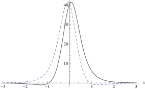
Figure 2: Plot of Morse potentials $V_{+}$ (solid line) and $V_{-}$ (dashed line) of Eq. (92), where we take $\hat{m}=0$, $D=5$, $\Lambda=1$, and $l=3$.

4 Concluding remarks

The $D$-dimensional Nariai spacetime studied in Section 3 is uncharged. Notice that there is a charged generalization of the $D$-dimensional Nariai spacetime, only we need to replace the quantity $\sigma$ of formula (42) by [8], [40]

$$\sigma_{Q}=(D-1)\Lambda-\frac{(D-3)^{2}Q^{2}}{a^{2(D-2)}},$$ (93)

and the parameter $a$ of expression (43) is replaced in the charged case by $a_{Q}$ which is a solution to the equation

$$\frac{(D-3)}{a_{Q}^{2}}=(D-1)\Lambda+\frac{(D-3)Q^{2}}{a_{Q}^{2(D-2)}},$$ (94)

where $Q$ is related to the electric charge of the spacetime.

Supported in our mathematical analysis of the problem for the uncharged Nariai spacetime, we assert that in the charged $D$-dimensional Nariai spacetime the QNF of the uncharged Dirac field are determined by formulae (86), only we must replace in these formulae the values of the quantities $\sigma$ and $a$ by $\sigma_{Q}$ and $a_{Q}$, respectively.

For identical values of the parameters $D$, $\Lambda$, and $n$, Morse potentials (92) and Pöschl-Teller potentials (91) have QNF with identical imaginary parts, that is with identical decay times, even when for identical values of $D$, $\Lambda$, and $l$ the height of Pöschl-Teller potential is smaller than the height of Morse potentials (see Figures 1 and 2). We believe that to find the source of this coincidence is an interesting question.

Also, in Ref. [49] was shown that for sufficiently late times the radial functions of Pöschl-Teller potential (91) form a complete basis. Owing to similarity of the plots for both potentials (see again Figures 1 and 2), to study if a similar result is valid for Morse potential (92) deserves a detailed investigation.

As we previously comment a similar reduction to that of Section 2 works for charged Dirac fields propagating in the $D$-dimensional charged spherically symmetric spacetimes [11]. We believe that a good exercise is to calculate the QNF of the charged Dirac field propagating in the $D$-dimensional charged Nariai spacetime to extend the results of Refs. [38], [39] and the previous section.

As we observe in Introduction section, the results on the separability of the Dirac equation in the four-dimensional Kerr black hole generalize to some $D$-dimensional rotating black holes [9], [13]. We believe that the extension of the results obtained in these references to the metrics of Plebanski-Demianski-Klemm type [50] deserve a detailed analysis. Furthermore the study of the separability properties of the equations of motion for gravitational and electromagnetic perturbations in the $D$-dimensional Myers-Perry metrics of Ref. [51] is a relevant problem.

5 Acknowledgements

I thank Dr. C. E. Mora Ley, Dr. R. García Salcedo, Dr. O. Pedraza Ortega and A. Tellez Felipe for their interest in this paper. This work was supported by CONACYT México, SNI México, EDI-IPN, COFAA-IPN, and Research Project SIP-20090952.

References

- [1] J. Polchinski, String Theory, Cambridge University Press, Cambridge, United Kingdom, (1998).
- [2] R. Emparan and H. S. Reall, Living Rev. Rel. 11, 6 (2008) [arXiv:0801.3471 [hep-th]].
- [3] K. D. Kokkotas and B. G. Schmidt, Living Rev. Rel. 2, 2 (1999) [arXiv:gr-qc/9909058]; E. Berti, V. Cardoso and A. O. Starinets, arXiv:0905.2975 [gr-qc]; H. P. Nollert, Class. Quantum Grav. 16, R159 (1999).
- [4] S. Chandrasekhar, The Mathematical Theory of Black Holes, Oxford University Press, Oxford (1983).
- [5] S. Hod, Phys. Rev. Lett. 81 (1998) 4293 [arXiv:gr-qc/9812002]; O. Dreyer, Phys. Rev. Lett. 90 (2003) 081301 [arXiv:gr-qc/0211076].
- [6] H. Kodama and A. Ishibashi, Prog. Theor. Phys. 110 (2003) 701 [arXiv:hep-th/0305147].
- [7] A. Ishibashi and R. M. Wald, Class. Quant. Grav. 20 (2003) 3815 [arXiv:gr-qc/0305012].
- [8] H. Kodama and A. Ishibashi, Prog. Theor. Phys. 111 (2004) 29 [arXiv:hep-th/0308128].
- [9] W. G. Unruh, Phys. Rev. D 10, 3194 (1974); W. G. Unruh, Phys. Rev. Lett. 31, 1265 (1973).
- [10] M. Martellini and A. Treves, Phys. Rev. D 15, 3060 (1977); B. R. Iyer and A. Kumar, Phys. Rev. D 18, 4799 (1978).
- [11] G. W. Gibbons and A. R. Steif, Phys. Lett. B 314, 13 (1993) [arXiv:gr-qc/9305018]; S. R. Das, G. W. Gibbons and S. D. Mathur, Phys. Rev. Lett. 78, 417 (1997) [arXiv:hep-th/9609052].
- [12] I. I. Cotaescu, Mod. Phys. Lett. A 13, 2991 (1998) [arXiv:gr-qc/9808030]; I. I. Cotăescu, Int. J. Mod. Phys. A 19, 2217 (2004) [arXiv:gr-qc/0306127].
- [13] S. Chandrasekhar, Proc. Roy. Soc. Lond. A 349, 571 (1976); D. N. Page, Phys. Rev. D 14, 1509 (1976); C. H. Lee, Phys. Lett. B 68, 152 (1977); T. Oota and Y. Yasui, Phys. Lett. B 659, 688 (2008) [arXiv:0711.0078 [hep-th]]; S. Q. Wu, Phys. Rev. D 78, 064052 (2008) [arXiv:0807.2114 [hep-th]]; S. Q. Wu, Class. Quant. Grav. 26, 055001 (2009) [arXiv:0808.3435 [hep-th]].
- [14] D. Kubiznak, arXiv:0809.2452 [gr-qc].
- [15] G. W. Gibbons, M. Rogatko and A. Szyplowska, Phys. Rev. D 77, 064024 (2008) [arXiv:0802.3259 [hep-th]]; G. W. Gibbons and M. Rogatko, Phys. Rev. D 77, 044034 (2008) [arXiv:0801.3130 [hep-th]].
- [16] H. T. Cho, A. S. Cornell, J. Doukas and W. Naylor, Phys. Rev. D 75, 104005 (2007) [arXiv:hep-th/0701193].
- [17] H. T. Cho, A. S. Cornell, J. Doukas and W. Naylor, Phys. Rev. D 77, 041502 (2008) [arXiv:0710.5267 [hep-th]].
- [18] D. J. Hurley and M. A. Vandick, Geometry, Spinors and Applications, Springer Praxis Publishing, Chichester (2000).
- [19] A. Van Proeyen, arXiv:hep-th/9910030.
- [20] P. C. West, arXiv:hep-th/9811101.
- [21] V. Cardoso and J. P. S. Lemos, Phys. Rev. D 63 (2001) 124015 [arXiv:gr-qc/0101052].
- [22] D. Birmingham, I. Sachs and S. N. Solodukhin, Phys. Rev. Lett. 88 (2002) 151301 [arXiv:hep-th/0112055].
- [23] J. Crisostomo, S. Lepe and J. Saavedra, Class. Quant. Grav. 21 (2004) 2801 [arXiv:hep-th/0402048].
- [24] S. Fernando, Gen. Rel. Grav. 36 (2004) 71 [arXiv:hep-th/0306214].
- [25] S. Fernando, Phys. Rev. D 77 (2008) 124005 [arXiv:0802.3321 [hep-th]].
- [26] S. Fernando, arXiv:0903.0088 [hep-th].
- [27] A. López-Ortega, Gen. Rel. Grav. 37 (2005) 167.
- [28] R. Becar, S. Lepe and J. Saavedra, Phys. Rev. D 75 (2007) 084021 [arXiv:gr-qc/0701099].
- [29] A. Lopez-Ortega, arXiv:0905.0073 [gr-qc].
- [30] A. López-Ortega, Gen. Rel. Grav. 38 (2006) 743 [arXiv:gr-qc/0605022].
- [31] D. P. Du, B. Wang and R. K. Su, Phys. Rev. D 70 (2004) 064024 [arXiv:hep-th/0404047].
- [32] A. López-Ortega, Gen. Rel. Grav. 38 (2006) 1565 [arXiv:gr-qc/0605027].
- [33] A. López-Ortega, Gen. Rel. Grav. 39, 1011 (2007) [arXiv:0704.2468 [gr-qc]].
- [34] J. Natario and R. Schiappa, Adv. Theor. Math. Phys. 8 (2004) 1001 [arXiv:hep-th/0411267].
- [35] L. h. Liu and B. Wang, Phys. Rev. D 78, 064001 (2008) [arXiv:0803.0455 [hep-th]].
- [36] R. Aros, C. Martinez, R. Troncoso and J. Zanelli, Phys. Rev. D 67 (2003) 044014 [arXiv:hep-th/0211024].
- [37] D. Birmingham and S. Mokhtari, Phys. Rev. D 74 (2006) 084026 [arXiv:hep-th/0609028].
- [38] A. Lopez-Ortega, Gen. Rel. Grav. 40, 1379 (2008) [arXiv:0706.2933 [gr-qc]].
- [39] L. Vanzo and S. Zerbini, Phys. Rev. D 70, 044030 (2004) [arXiv:hep-th/0402103].
- [40] H. Nariai, Sci. Rep. Tohoku Univ., First Ser. 34, 160 (1950). Reproduced in H. Nariai, Gen. Rel. Grav. 31, 951 (1999); H. Nariai, Sci. Rep. Tohoku Univ., First Ser. 35, 46 (1951). Reproduced in H. Nariai, Gen. Rel. Grav. 31, 963 (1999).
- [41] S. Winitzki, Advanced General Relativity. Lecture notes, version 1.1, dated September 28, 2007. Avaible in http://homepages.physik.uni-muenchen.de/Winitzki/ (consulted at February 28, 2009).
- [42] M. Nakahara, Geometry, Topology and Physics, Institute of Physics Publishing, Bristol (1992); T. Frankel, The Geometry of Physics. An Introduction, Cambridge University Press, Cambridge (1997).
- [43] L. Vanzo, Phys. Rev. D 56, 6475 (1997) [arXiv:gr-qc/9705004]; D. Birmingham, Class. Quant. Grav. 16, 1197 (1999) [arXiv:hep-th/9808032]; J. P. S. Lemos, Phys. Lett. B 353, 46 (1995) [arXiv:gr-qc/9404041].
- [44] R. Camporesi and A. Higuchi, J. Geom. Phys. 20, 1 (1996) [arXiv:gr-qc/9505009].
- [45] A. Lopez-Ortega, Gen. Rel. Grav. 36, 1299 (2004).
- [46] M. Abramowitz and I. A. Stegun, Handbook of Mathematical Functions, Graphs, and Mathematical Table, Dover Publications, New York (1965); Z. X. Wang and D. R. Guo, Special Functions, World Scientific Publishing, Singapore (1989).
- [47] V. Ferrari and B. Mashhoon, Phys. Rev. Lett. 52, 1361, (1984).
- [48] R. Dutt, A. Khare and U. P. Sukhatme, Am. J. Phys. 56, 163, (1988)
- [49] H. R. Beyer, Commun. Math. Phys. 204, 397 (1999) [arXiv:gr-qc/9803034].
- [50] D. Klemm, JHEP 9811, 019 (1998) [arXiv:hep-th/9811126]; A. Lopez-Ortega, Gen. Rel. Grav. 35, 1785 (2003); Z. W. Chong, G. W. Gibbons, H. Lu and C. N. Pope, Phys. Lett. B 609, 124 (2005) [arXiv:hep-th/0405061].
- [51] R. C. Myers and M. J. Perry, Annals Phys. 172, 304 (1986).