Regge poles of the Schwarzschild black hole: a WKB approach

Abstract

We provide simple and accurate analytical expressions for the Regge poles of the Schwarzschild black hole. This is achieved by using third-order WKB approximations to solve the radial wave equations for spins 0, 1, and 2. These results permit us to obtain analytically the dispersion relation and the damping of the “surface waves” lying close to the photon sphere of the Schwarzschild black hole and which generate the weakly damped quasinormal modes of its spectrum. Our results could be helpful in order to simplify considerably the description of wave scattering from the Schwarzschild black hole as well as the analysis of the gravitational radiation created in many black hole processes. Furthermore, the existence of nonlinear dispersion relations for the photons propagating close to the photon sphere could have also important consequences in the context of gravitational lensing.

I Introduction

Since the sixties, mainly under the impetus of Nussenzveig in electromagnetism and Regge in quantum physics, asymptotic/semiclassical techniques which use analytic continuation of partial-wave representations have been developed to understand scattering theory and the associated resonance phenomenons. Together these techniques form the complex angular momentum (CAM) method. The CAM method originates from the pioneering work of Watson Watson (1918) dealing with the propagation and diffraction of radio waves around the earth (see also the modification proposed by Sommerfeld Sommerfeld (1949) of the Watson approach). Today, the CAM method has been successfully introduced in various domains of physics. For reviews of the CAM method we refer to the monographs of Newton Newton (1982), Nussenzveig Nussenzveig (1992), Grandy W. T. Grandy (2000), Collins Collins (1977) and Gribov Gribov (2003) as well as to references therein for various applications in quantum mechanics, nuclear physics, particle and high-energy physics, electromagnetism, optics, and seismology.

The CAM method is based on the dual structure of the $S$-matrix associated with a given scattering problem. Indeed, the $S$-matrix is a function of both the frequency $\omega$ and the angular momentum index $\ell$. It can be analytically extended into the complex $\omega$ plane as well as into the complex $\ell$ plane (CAM plane). Its poles lying in the fourth quadrant of the complex $\omega$ plane are the complex frequencies of the resonant modes. In other words, the behavior of the $S$-matrix in the complex $\omega$ plane permits us to investigate resonance phenomenons. The structure of the $S$-matrix in the complex $\ell$ plane allows us – by using integration contour deformations, Cauchy’s Theorem, and asymptotic analysis – to provide a semiclassical description of scattering in terms of geometric and diffractive rays. In that context, the poles of the $S$-matrix lying in the first quadrant of the CAM plane (the so-called Regge poles) are associated with diffraction. Of course, when a connection between these two faces of the $S$-matrix can be established, resonance aspects of scattering are then semiclassically interpreted.

More precisely, for spherically symmetric scattering problems, the connection between the resonant approach of scattering and its Regge pole interpretation is a consequence of the following considerations:

i) For a given value $\ell\in{\bf N}$ of the angular momentum index, the resonances, i.e., the complex poles of the matrix element $S_{\ell}(\omega)$, are of the form $\omega_{\ell n}=\omega^{(o)}_{\ell n}-i\Gamma_{\ell n}/2$, where $n\in{\bf N}$ and, in the immediate neighborhood of $\omega_{\ell p}$, $S_{\ell}(\omega)$ has the Breit-Wigner form, i.e.,

$$S_{\ell}(\omega)\propto\frac{\Gamma_{\ell n}/2}{\omega-\omega^{(o)}_{\ell n}+i\Gamma_{\ell n}/2}.$$ (1)

ii) For a given value $\omega>0$ of the frequency, the Regge poles, i.e., the complex poles of the matrix element $S_{\lambda-1/2}(\omega)$, can be expressed as function of the form $\lambda_{n}(\omega)$. The curves traced out in the CAM plane by the Regge poles as a function of the frequency $\omega$ are the so-called Regge trajectories. They permit us to interpret Regge poles in terms of diffractive rays or “surface waves”: $\mathrm{Re}\,\lambda_{n}(\omega)$ provides the dispersion relation for the $n$th “surface wave”, while $\mathrm{Im}\,\lambda_{n}(\omega)$ corresponds to its damping.

(iii) From the Regge trajectories, we can semiclassically construct the resonance spectrum. There exists a first semiclassical formula (a Bohr-Sommerfeld-type quantization condition) which provides the location of the excitation frequencies $\omega^{(0)}_{\ell n}$ of the resonances generated by $n$th “surface wave”:

$$\mathrm{Re}\,\lambda_{n}\left(\omega^{(0)}_{\ell n}\right)=\ell+1/2,\qquad\ell\in{\bf N}.$$ (2)

There exists a second semiclassical formula which provides the widths of these resonances

$$\frac{\Gamma_{\ell n}}{2}=\left.\frac{\mathrm{Im}\,\lambda_{n}(\omega)[d/d\omega\,\mathrm{Re}\,\lambda_{n}(\omega)]}{[d/d\omega\,\mathrm{Re}\,\lambda_{n}(\omega)]^{2}+[d/d\omega\,\mathrm{Im}\,\lambda_{n}(\omega)]^{2}}\right|_{\omega=\omega^{(0)}_{\ell n}}$$ (3)

and which reduces, in the frequency range where the condition $|d/d\omega\,\mathrm{Re}\,\lambda_{n}(\omega)|\gg|d/d\omega\,\mathrm{Im}\,\lambda_{n}(\omega)|$ is satisfied, to

$$\frac{\Gamma_{\ell n}}{2}=\left.\frac{\mathrm{Im}\,\lambda_{n}(\omega)}{d/d\omega\,\ \mathrm{Re}\,\lambda_{n}(\omega)}\right|_{\omega=\omega^{(0)}_{\ell n}}.$$ (4)

Recently, by using CAM techniques or in other words the Regge pole machinery, we have established that the weakly damped quasinormal mode (QNM) complex frequencies of the Schwarzschild black hole of mass $M$ are Breit-Wigner-type resonances generated by a family of “surface waves” lying on its photon sphere at $r=3M$ Décanini et al. (2003). More precisely, by noting that each “surface wave” is associated with a Regge pole of the $S$-matrix of the Schwarzschild black hole Andersson and Thylwe (1994); Andersson (1994); Décanini et al. (2003), we have been able to numerically construct the spectrum of the QNM complex frequencies from the associated Regge trajectories. In fact, in this way, from CAM methods, we have given meaning to an appealing and physically intuitive interpretation of the Schwarzschild black hole QNMs suggested by Goebel in 1972 Goebel (1972), i.e., that they could be interpreted in terms of gravitational waves in spiral orbits close to the unstable circular photon orbit at $r=3M$ which decay by radiating away energy. It should be noted that alternative implementations of the Goebel interpretation have been developed (see Refs. Ferrari and Mashhoon (1984); Mashhoon (1985); Stewart (1989); Andersson and Onozawa (1996); Zerbini and Vanzo (2004); Cardoso et al. (2009)) but they are mainly based on the concepts of geodesic and bundle of geometrical rays while our CAM analysis is based on wave physics.

In Sec. 2 of this short note, we provide analytical expressions for the Regge poles corresponding to the scalar field (spin 0), the electromagnetic field (spin 1) and the gravitational perturbations (spin 2) propagating on the Schwarzschild background. This is achieved by using the WKB approach developed in the context of the determination of the QNMs by Schutz and Will Schutz and Will (1985) and by Will and Iyer Iyer and Will (1987); Iyer (1987) (see also Ref. Bender and Orszag (1978) for general aspects of WKB theory and for particular aspects connected with eigenvalue problems of the type considered here). Our WKB results permit us to describe very accurately the Regge trajectories of the Schwarzschild black hole and to recover from the semiclassical formulas (2) and (4) well-known analytical expressions for the QNM complex frequencies. It should be noted that in Ref. Décanini et al. (2003), from numerical considerations, we have provided a coarse formula for the Regge poles of the Schwarzschild black hole. It has been sufficient in order to obtain a “surface wave” interpretation of the QNM complex frequencies but it does not take into account the spin dependent aspects of the problem as well as the fact that (i) the dispersion relation of the $n$th “surface wave” is nonlinear and depends on the index $n$ and that (ii) the damping of the $n$th “surface wave” is frequency dependent. In the present paper, we have derived analytical expressions for the Regge poles of the Schwarzschild black hole from mathematical considerations. The results displayed in Ref. Décanini et al. (2003) are the leading-order counterpart for very high frequencies of our new results which are much more accurate and which now permit us to describe precisely the behavior of the Regge poles and of the associated “surface waves” in a very large range of frequencies. In Sec. 3, we briefly conclude by considering some possible consequences and applications of our results.

II Regge poles, Regge trajectories, and WKB results

The wave equations for the scalar field, for the electromagnetic field, and for the gravitational perturbations propagating on the Schwarzschild black hole reduce, after separation of variables, to the Regge-Wheeler equation (a one-dimensional Schrödinger equation)

$$\frac{d^{2}\Phi_{\ell}}{dr_{*}^{2}}+\left[\omega^{2}-V_{\ell}(r)\right]\Phi_{\ell}=0$$ (5)

where the effective potential $V_{\ell}(r)$ is given by

$$V_{\ell}(r)=\left(\frac{r-2M}{r}\right)\left[\frac{\ell(\ell+1)}{r^{2}}+\frac{2(1-s^{2})M}{r^{3}}\right].$$ (6)

Here, $s$ denotes the spin of the field considered, $\ell\in{\bf N}$ is the ordinary angular momentum index, while $r$ and $r_{*}=r+2M\ln\left(r/2M-1\right)+\mathrm{const}$ are, respectively, the standard radial Schwarzschild coordinate and the Regge-Wheeler tortoise coordinate, and we have furthermore assumed a harmonic time dependence $e^{-i\omega t}$.

For a given angular momentum index $\ell$, the $S$-matrix element $S_{\ell}(\omega)$ is obtained by seeking the solutions of the Regge-Wheeler equation (5) which have a purely ingoing behavior at the event horizon $r=2M$, i.e. which satisfy

$$\Phi_{\ell}(r)\underset{r_{*}\to-\infty}{\sim}e^{-i\omega r_{*}}$$ (7)

and which, at spatial infinity $r\to+\infty$, have an asymptotic behavior of the form

$$\Phi_{\ell}(r)\underset{r_{*}\to+\infty}{\sim}\frac{1}{T_{\ell}(\omega)}e^{-i\omega r_{*}+i\ell\pi/2}-\frac{S_{\ell}(\omega)}{T_{\ell}(\omega)}e^{+i\omega r_{*}-i\ell\pi/2}.$$ (8)

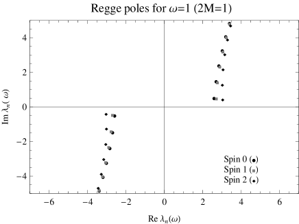
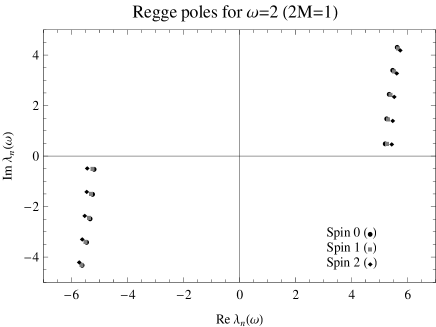
Figure 1: Regge pole distributions for $\omega=1$ and $\omega=2$ ($2M=1$). Scalar and electromagnetic fields as well as gravitational perturbations are considered.

For $\omega>0$, the Regge poles of the $S$-matrix are the complex values $\lambda$ for which, both $S_{\lambda-1/2}(\omega)$ and $T_{\lambda-1/2}(\omega)$ have a simple pole but $S_{\lambda-1/2}(\omega)/T_{\lambda-1/2}(\omega)$ is regular Décanini et al. (2003). They constitute a family $\lambda_{n}(\omega)$ with the index $n=1,2,\dots$ permitting us to distinguish between the different poles. The corresponding modes are the solutions of the radial wave equation (5) which are purely outgoing at infinity and purely ingoing at the horizon. They are the “Regge modes” of the Schwarzschild black hole. It should be noted that the QNMs of the Schwarzschild black hole and the associated complex frequencies are defined in an analogous way with moreover a fundamental difference. Indeed, they are obtained for fixed values of $\ell\in{\bf N}$ and exist only for complex values of $\omega$.

In Ref. Décanini et al. (2003), we have noted that the Regge poles can be determined by using, mutatis mutandis, the method developed by Leaver Leaver (1985) for the search of the QNM complex frequencies and we have furthermore numerically implemented this method from the Hill determinant approach of Majumdar and Panchapakesan Majumdar and Panchapakesan (1989). For the Regge poles lying close to the real axis of the CAM plane, the “exact” results we can obtain numerically are accurate ones. Figure 1 exhibits the distribution of Regge poles for two different values of the frequency $\omega$. On this figure, the splitting of the Regge poles with the spin $s$ and the index $n$ as well as the migration of the first Regge poles corresponding to spins 0, 1 and 2 can be observed. This migration can be more precisely described by studying the Regge trajectories, i.e., the curves traced out in the CAM plane by the functions $\lambda_{n}(\omega)$ for $\omega\in[0,+\infty[$. In Figs. 2-4 we have displayed the Regge trajectories for the first three Regge poles associated with the scalar field, the electromagnetic field and the gravitational perturbations. As we have already noted in Ref. Décanini et al. (2003), $\mathrm{Re}\,\lambda_{n}(\omega)$ and $\mathrm{Im}\,\lambda_{n}(\omega)$ respectively denote the azimuthal propagation constant (i.e., the dispersion relation) and the damping constant of the $n$th “surface wave” lying on the photon sphere. So Figs. 2-4 permit us to note that, at first sight, (i) the global behavior of these “surface waves” is rather independent of the spin considered (such result is only valid for high frequencies) and (ii) for a given spin, the dispersion relation seems to be independent of the “surface wave” considered (such result is also only valid for high frequencies) and the “surface wave” corresponding to the first Regge pole has the weakest attenuation and therefore must play the most important role in scattering and in radiative processes and must contribute significantly to the resonance mechanism.

Figure 2: Regge trajectories for the scalar field. The Regge poles $\lambda_{n}(\omega)$ ($n=1,2,3$) are followed for $\omega=0\to 5$ ($2M=1$).

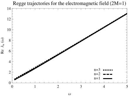
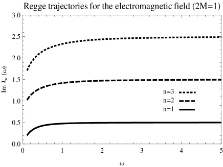
Figure 3: Regge trajectories for the electromagnetic field. The Regge poles $\lambda_{n}(\omega)$ ($n=1,2,3$) are followed for $\omega=0\to 5$ ($2M=1$).

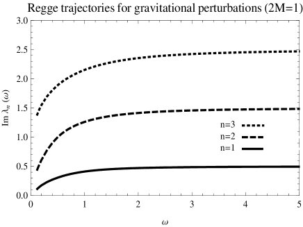
Figure 4: Regge trajectories for gravitational perturbations. The Regge poles $\lambda_{n}(\omega)$ ($n=1,2,3$) are followed for $\omega=0\to 5$ ($2M=1$).

The WKB approach developed in the context of the determination of the QNMs by Schutz and Will Schutz and Will (1985) and by Will and Iyer Iyer and Will (1987); Iyer (1987) (see also Ref. Bender and Orszag (1978)) can be easily adapted in order to obtain analytical approximations for the Regge poles. Indeed, as we have already noted, Regge modes and QNMs both satisfy the same wave equation and the same boundary conditions but with different interpretations for the angular momentum index and the frequency. By using third-order WKB approximations Iyer and Will (1987); Iyer (1987) for the Regge modes, we can find that the Regge poles $\lambda$ are the complex solutions of the equation

$$\omega^{2}=\left[V_{0}(\lambda)+{[-2V_{0}^{(2)}(\lambda)]}^{1/2}\,{\overline{\Lambda}}(\lambda,n)\right]$$

$$\qquad-i\,\alpha(n)\,{[-2V_{0}^{(2)}(\lambda)]}^{1/2}[1+{\overline{\Omega}}(\lambda,n)]$$ (9)

with $\omega>0$ and $n=1,2,3,\dots$. Here

$${\overline{\Lambda}}(\lambda,n)=\frac{1}{{[-2V_{0}^{(2)}(\lambda)]}^{1/2}}\left[\frac{1}{8}\frac{V_{0}^{(4)}(\lambda)}{V_{0}^{(2)}(\lambda)}\left(\frac{1}{4}+\alpha(n)^{2}\right)\right.$$

$$\qquad\left.-\frac{1}{288}\left(\frac{V_{0}^{(3)}(\lambda)}{V_{0}^{(2)}(\lambda)}\right)^{2}\left(7+60\,\alpha(n)^{2}\right)\right]$$ (10a)

and

$${\overline{\Omega}}(\lambda,n)=\frac{1}{[-2V_{0}^{(2)}(\lambda)]}\times$$

$$\qquad\left[\frac{5}{6912}\left(\frac{V_{0}^{(3)}(\lambda)}{V_{0}^{(2)}(\lambda)}\right)^{4}\left(77+188\,\alpha(n)^{2}\right)\right.$$

$$\qquad\left.-\frac{1}{384}\left(\frac{{[V_{0}^{(3)}(\lambda)]}^{2}V_{0}^{(4)}(\lambda)}{{[V_{0}^{(2)}(\lambda)]}^{3}}\right)\left(51+100\,\alpha(n)^{2}\right)\right.$$

$$\qquad\left.+\frac{1}{2304}\left(\frac{V_{0}^{(4)}(\lambda)}{V_{0}^{(2)}(\lambda)}\right)^{2}\left(67+68\,\alpha(n)^{2}\right)\right.$$

$$\qquad\left.+\frac{1}{288}\left(\frac{V_{0}^{(3)}(\lambda)V_{0}^{(5)}(\lambda)}{{[V_{0}^{(2)}(\lambda)]}^{2}}\right)\left(19+28\,\alpha(n)^{2}\right)\right.$$

$$\qquad\left.-\frac{1}{288}\left(\frac{V_{0}^{(6)}(\lambda)}{V_{0}^{(2)}(\lambda)}\right)\left(5+4\,\alpha(n)^{2}\right)\right].$$ (10b)

In Eqs. (II) and (10), we have introduced the notations

$$\alpha(n)=n-1/2$$ (11a)

and, for $$p\in{\bf N}$$,

$$V_{0}^{(p)}(\lambda)=\left.\frac{d^{p}}{{dr_{*}}^{p}}V_{\lambda-1/2}(r_{*})\right|_{r_{*}={(r_{*})}_{0}}$$ (11b)

with ${(r_{*})}_{0}$ which denotes the maximum of the function $V_{\lambda-1/2}(r_{*})$. We can solve Eq. (II) by assuming $|\lambda|\gg 1$ as well as $\mathrm{Re}\,\lambda\gg\mathrm{Im}\,\lambda$. Its solutions constitute a family $\lambda_{n}(\omega)$ with $n=1,2,3,\dots$, and we have the approximation

$$\lambda_{n}(\omega)\approx{[27(M\omega)^{2}+a_{n}+2(n-1/2)^{2}\epsilon_{n}(\omega)]}^{1/2}$$

$$\qquad\qquad+i\,(n-1/2)[1+\epsilon_{n}(\omega)]$$ (12)

where

$$a_{n}=\frac{2}{3}\left[\frac{5}{12}(n-1/2)^{2}+\frac{115}{144}-1+s^{2}\right]$$ (13)

and

$$\epsilon_{n}(\omega)=\frac{b_{n}}{27(M\omega)^{2}+a_{n}+(n-1/2)^{2}}$$ (14)

with

$$b_{n}=-\frac{4}{9}\left[\frac{305}{1728}(n-1/2)^{2}+\frac{5555}{6912}-1+s^{2}\right].$$ (15)

Equation (II) is the main result of our paper. It also provides expressions for the dispersion relation and the damping of the “surface waves” lying on/close the photosphere of the Schwarzschild black hole. It is important to note that the perturbation parameter of the WKB method leading to Eq. (II) is not $1/\omega$ with $\omega\to+\infty$ but, in some sense, the distance $\epsilon^{1/2}$ (with formally $\epsilon\to 0$) between the turning points of Eq. (5) [i.e., the roots of $Q(r^{\ast})=\omega^{2}-V_{\ell}(r^{\ast})$] and the location of the peak of $Q(r^{\ast})$ (see also Refs. Schutz and Will (1985); Iyer and Will (1987); Iyer (1987)). As a consequence, Eq. (II) is valid in a very large range of frequency values and not only for $\omega\to+\infty$. Of course, in order to solve Eq. (II) and to obtain the expression (II), we have furthermore assumed that $|\lambda|\gg 1$ as well as $\mathrm{Re}\,\lambda\gg\mathrm{Im}\,\lambda$. As a consequence, we can expect the accuracy to decrease for very low frequencies and for higher Regge poles.

Table 1: A sample of Regge pole values for the scalar field ($2M=1$): Exact versus WKB results.

		Exact	Exact	WKB	WKB
$n$	$\omega$	$\mathrm{Re}\,\lambda_{n}(\omega)$	$\mathrm{Im}\,\lambda_{n}(\omega)$	$\mathrm{Re}\,\lambda_{n}(\omega)$	$\mathrm{Im}\,\lambda_{n}(\omega)$
1	0.5	1.2828209	0.5159935	1.2809160	0.5180607
				(0.15 % )	( -0.40 % )
	1.0	2.5868446	0.5047360	2.5865154	0.5048769
				(0.013 % )	( -0.028 % )
	2.0	5.1900754	0.5012355	5.1900317	0.5012441
				(0.0008 % )	( -0.002 % )
	5.0	12.9878966	0.5002000	12.9878938	0.5002002
				(0.00002 % )	( -0.00004 % )
	8.0	20.7830530	0.5000782	20.7830523	0.5000783
				(0.000003 % )	( -0.00002 % )
2	0.5	1.4528181	1.4306871	1.4448341	1.4697683
				(0.55 % )	( -2.73 % )
	1.0	2.6883554	1.4795865	2.6829878	1.4858943
				(0.2 % )	( -0.43 % )
	2.0	5.2429941	1.4949257	5.2418734	1.4954987
				(0.02 % )	( -0.04 % )
	5.0	13.0092503	1.4992028	13.0091660	1.4992194
				(0.0006 % )	( -0.001 % )
	8.0	20.7964105	1.4996895	20.7963895	1.4996921
				(0.0001 % )	( -0.0002 % )
3	0.5	1.6413824	2.2423840	1.6616950	2.3943757
				(-1.24 % )	( -6.78 % )
	1.0	2.8430931	2.3914352	2.8296345	2.4309959
				(0.47 % )	( -1.65 % )
	2.0	5.3400891	2.4659363	5.3345383	2.4710894
				(0.10 % )	( -0.21 % )
	5.0	13.0513306	2.4941174	13.0507979	2.4942946
				(0.004 % )	( -0.007 % )
	8.0	20.8229704	2.4976812	20.8228335	2.4977092
				(0.0007 % )	( -0.001 % )

Table 2: A sample of Regge pole values for the electromagnetic field ($2M=1$): Exact versus WKB results.

		Exact	Exact	WKB	WKB
$n$	$\omega$	$\mathrm{Re}\,\lambda_{n}(\omega)$	$\mathrm{Im}\,\lambda_{n}(\omega)$	$\mathrm{Re}\,\lambda_{n}(\omega)$	$\mathrm{Im}\,\lambda_{n}(\omega)$
1	0.5	1.4815049	0.4253267	1.4883412	0.4258078
				(-0.46 % )	( -0.11 % )
	1.0	2.7053584	0.4754545	2.7068558	0.4752165
				(-0.06 % )	( 0.05 % )
	2.0	5.2528681	0.4932626	5.2531027	0.4932356
				(-0.004 % )	( 0.005 % )
	5.0	13.0134669	0.49889000	13.0134830	0.49888916
				(-0.0001 % )	( 0.0002 % )
	8.0	20.7990685	0.4995649	20.7990725	0.4995647
				(-0.00002 % )	( 0.00004 % )
2	0.5	1.5332591	1.3156541	1.5406267	1.3428745
				(-0.48 % )	( -2.07 % )
	1.0	2.7692625	1.4191713	2.7696511	1.4211866
				(-0.01 % )	( -0.14 % )
	2.0	5.2986954	1.4736965	5.2989080	1.4736729
				(-0.004 % )	( 0.002 % )
	5.0	13.0342937	1.4953538	13.0343184	1.4953500
				(-0.0002 % )	( 0.0003 % )
	8.0	20.8122949	1.4981621	20.8123014	1.4981614
				(-0.00003 % )	( 0.00005 % )
3	0.5	1.6777130	2.1559691	1.7082310	2.2924069
				(-1.82 % )	( -6.33 % )
	1.0	2.8922912	2.3300925	2.8852566	2.3612376
				(0.24 % )	( -1.34 % )
	2.0	5.3854965	2.4370870	5.3824034	2.4403495
				(0.06 % )	( -0.13 % )
	5.0	13.0753825	2.4879569	13.0751198	2.4880481
				(0.002 % )	( -0.004 % )
	8.0	20.8385991	2.4951766	20.8385333	2.4951904
				(0.0003 % )	( -0.006 % )

Table 3: A sample of Regge pole values for gravitational perturbations ($2M=1$): Exact versus WKB results.

		Exact	Exact	WKB	WKB
$n$	$\omega$	$\mathrm{Re}\,\lambda_{n}(\omega)$	$\mathrm{Im}\,\lambda_{n}(\omega)$	$\mathrm{Re}\,\lambda_{n}(\omega)$	$\mathrm{Im}\,\lambda_{n}(\omega)$
1	0.5	1.9892654	0.3065938	2.0250887	0.3116324
				(-1.80 % )	( -1.64 %)
	1.0	3.0310943	0.4112060	3.0434848	0.4109477
				(-0.41 % )	( 0.06 % )
	2.0	5.4358037	0.4714533	5.4381254	0.4713563
				(-0.04 % )	( 0.02 % )
	5.0	13.0897823	0.4950209	13.0899530	0.4950172
				(-0.001 % )	( 0.0007 % )
	8.0	20.8470170	0.4980343	20.8470594	0.4980337
				(-0.0002 % )	( 0.0001 % )
2	0.5	1.8354561	0.9996004	1.9133037	1.1052746
				(-4.24 % )	( -10.57 % )
	1.0	3.0182689	1.2608708	3.0358421	1.2696433
				(-0.58 % )	( -0.70 % )
	2.0	5.4634287	1.4143591	5.4679208	1.4135833
				(-0.08 % )	( 0.05 % )
	5.0	13.1090753	1.4839779	13.1095067	1.4839195
				(-0.003 % )	( 0.004 % )
	8.0	20.8598549	1.4936074	20.8599664	1.4935974
				(-0.0005 % )	( 0.0007 % )
3	0.5	1.806641	1.888817	1.929425	2.053332
				(-6.80 % )	( -8.71 % )
	1.0	3.0504514	2.1517280	3.0724443	2.1842791
				(-0.72 % )	( -1.51 % )
	2.0	5.5221237	2.3542390	5.5264762	2.3546842
				(-0.08 % )	( -0.02 % )
	5.0	13.1472705	2.4697252	13.1478689	2.4695873
				(-0.005 % )	( 0.006 % )
	8.0	20.8854004	2.4877063	20.8855672	2.4876795
				(-0.0008 % )	( 0.001 % )

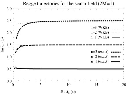
Figure 5: Regge trajectories spins 0, 1 and 2: Exact versus WKB calculations. For the Regge poles $\lambda_{n}(\omega)$ ($n=1,2,3$) followed for $\omega=0\to 8$ ($2M=1$), $\mathrm{Im}\,\lambda_{n}(\omega)$ is expressed as a function of $\mathrm{Re}\,\lambda_{n}(\omega)$.

Tables 1-3 present a sample of Regge pole positions calculated from the WKB result (II). The WKB results are better for high frequencies and for the first Regge pole. However, a comparison between the “exact” and the WKB results shows a good agreement even for low frequencies and for the second and third Regge poles. Formula (II) permit us also to describe very accurately the Regge trajectories of the Schwarzschild black hole [see Fig. 5 where, for clarity, we have considered the Regge trajectories in the form $\mathrm{Im}\,\lambda_{n}(\omega)$ as a function of $\mathrm{Re}\,\lambda_{n}(\omega)$]. It should be also noted that, in Ref. Glampedakis and Andersson (2003), Glampedakis and Andersson have developed a “quick and dirty” method which provides very accurate results for the Regge poles (see Table 4 in their article where the first three Regge poles associated with the scalar field are given). Their numerical method is certainly better than the WKB method we have considered. But it is only a purely numerical method used in order to approximate the exact results. Our WKB approach permits us to provide a simple and accurate analytical expression for the Regge poles. It would be also possible to improve considerably our WKB results by adapting the higher order WKB approach developed by Konoplya in Ref. Konoplya (2003). But we believe that the Konoplya approach could not provide a formula as simple as (II).

Figure 6: Regge trajectories (spin 2, $n=1$): Exact versus WKB calculations. The Regge pole $\lambda_{1}(\omega)$ followed for $\omega=0.12\to 1.83$ ($2M=1$).

It is moreover possible to simplify (II) and to write

$$\lambda_{n}(\omega)=\left[3\sqrt{3}\,M\omega+\frac{\sqrt{3}\,a_{n}}{18M\omega}\right]$$

$$\qquad+i\left(n-1/2\right)\left[1+\frac{b_{n}}{27(M\omega)^{2}}\right]+\underset{\omega\to+\infty}{\cal O}\left(\frac{1}{\omega^{3}}\right)$$

which is much more elegant. Of course, this alternative formula provides accurate results only at large $\omega$ and must not be used at low frequencies (see Fig. 6). It provides very simple expressions for the dispersion relation and the damping of the “surface waves” lying on the photosphere of the Schwarzschild black hole. The leading-order terms of Eq. (II) correspond to the expression (19) of Ref. Décanini et al. (2003). Of course, this expression is too coarse to take into account precisely the spin and index dependence which appear clearly in Fig. 1 and, furthermore, it does not emphasize the nonlinear behavior of the dispersion relations as well as the nonconstant behavior of the damping (see Figs. 2-4). As a consequence, the numerical calculations which use it are not accurate for low frequencies $\omega$, for high indices $n$ and for high spins $s$. For example, for $2M=1$, $\omega=1$, $n=3$, and $s=0$, the formula (19) of Ref. Décanini et al. (2003) leads to important errors about $8.6~{}\%$ for the real part of the Regge pole and $-4.5~{}\%$ for its imaginary part. For $s=1$ the errors are, respectively, about $10.0~{}\%$ and $-7.3~{}\%$, and for $s=2$ they are about $14.8~{}\%$ and $-16.2~{}\%$.

In a recent paper Dolan and Ottewill (2009) written after the first version of the present one, Dolan and Ottewill have greatly improved our high frequency approximation (II) by providing higher orders in $1/\omega$. But, as they have noted, their expansion is not as accurate as our formula (II) in the low-$\omega$ regime. This reinforces again our view that Eq. (II) is a very interesting result due to its large range of validity.

In Ref. Décanini et al. (2003), we have proven that the “surface waves” associated with the family of Regge poles propagate on the photon sphere of the Schwarzschild black hole at $r=3M$. We have established this connection by using the leading-order behavior of (II). It is therefore a semiclassical interpretation which is formally valid for $\omega\to+\infty$. In this context, we recall (see Ref. Décanini et al. (2003)) that the resonant part of the form factor of the Schwarzschild black hole is a superposition of terms like $\exp[i(\lambda_{n}(\omega)\theta-\omega t)]$ which can be also written in the form

$$\exp[-k^{\prime\prime}_{n}(\omega){\cal L}]\exp[i(k^{\prime}_{n}(\omega){\cal L}-\omega t)]$$ (17)

with ${\cal L}=(3M)\theta$ which denotes the arc length taken on the photon sphere. Here $k^{\prime}_{n}(\omega)=\mathrm{Re}\,\lambda_{n}(\omega)/(3M)$ represents the wavenumber of the $n$th “surface wave” lying on the photon sphere, or in other terms its dispersion relation, while $k^{\prime\prime}_{n}(\omega)=\mathrm{Im}\,\lambda_{n}(\omega)/(3M)$ is its damping constant. To the leading order, the dispersion relation is linear but if we go beyond this order, it is clearly nonlinear [see Eqs. (II) and (II)], and this last result could have important consequences in strong gravitational lensing. But the previous analysis could be also inexact: indeed, if we need to take into account the finite value of the photon frequency, the nonlinear corrections could also induce a shift for the location of the unstable circular orbit of the photon and it would be then necessary to slightly modify (17) and more particularly the expression of the arc length ${\cal L}$.

Finally, let us note that our WKB results permit us to recover from the semiclassical formulas (2) and (4) well-known analytical expressions for the QNM complex frequencies. Indeed, by inserting (II) into Eqs. (2) and (4), we obtain the well-known large $\ell$ behaviors [see Eq. (3.1) of Ref. Iyer (1987)]

$$\omega^{(o)}_{\ell n}=\frac{1}{3\sqrt{3}M}\left[(\ell+1/2)-\frac{a_{n}}{2\ell}+\frac{a_{n}}{4\ell^{2}}+\underset{\ell\to+\infty}{\cal O}\left(\frac{1}{\ell^{3}}\right)\right]$$

(18a)

$$\frac{\Gamma_{\ell n}}{2}=\frac{n-1/2}{3\sqrt{3}M}\left[1+\frac{c_{n}}{2\ell^{2}}+\underset{\ell\to+\infty}{\cal O}\left(\frac{1}{\ell^{3}}\right)\right]$$ (18b)

with $\ell\in{\bf N}$ and $n=1,2,\dots$. Here,

$$c_{n}=a_{n}+2b_{n}=-\frac{2}{9}\left[-\frac{235}{432}(n-1/2)^{2}+\frac{1415}{1728}-1+s^{2}\right].$$ (19)

Here, it is worth recalling that the leading order of (18) can be expressed in terms of the angular velocity at the unstable circular null geodesic, i.e. at $r=3M$, while the leading order of (18b) is related to the corresponding Lyapunov exponent (see Ref. Cardoso et al. (2009)).

III Conclusion

The success of the CAM method in physics is due to its ability to provide a clear description of a given scattering problem by extracting the physical information (linked to the geometrical and diffractive aspects of the scattering process) which is hidden in partial-wave representations. In the context of black hole physics, the CAM method has permitted us to clearly interpret the existence of the weakly damped QNM complex frequencies of the Schwarzschild black hole in terms of “surface waves” propagating on/close to its photon sphere Décanini et al. (2003); Andersson and Thylwe (1994); Andersson (1994) and, in the present paper, we have derived analytical expressions for the dispersion relation and the damping of these “surface waves” [see Eqs. (II) and (II)] or, equivalently, for the location in the CAM plane of the Regge poles of the Schwarzschild black hole associated with these “surface waves”.

The analytical expressions we have obtained for the Regge poles of the Schwarzschild black hole may be helpful in order to simplify considerably (i) the description of wave scattering from this gravitational background as well as (ii) the description of the gravitational radiation created in many black hole processes involving this gravitational background. In the former context, the approach initiated by Andersson and Thylwe Andersson and Thylwe (1994); Andersson (1994) is certainly the most promising way. In the latter one, a formalism based on the Regge pole machinery has not yet be developed and all the work remains to be done.

Our results could have also very important consequences and applications in the context of gravitational lensing. Indeed, until now the gravitational lens effects due to the Schwarzschild black hole have been only considered in the framework of geometrical optics where light propagation is described in terms of null geodesics. In this framework, photon dispersion is completely irrelevant. But, in the present paper, we have established from wave theoretical considerations the existence of dispersion relations for the photons propagating close to the photon sphere at $r=3M$ and it is well-known that this “surface plays” a crucial role in the context of the strong-deflection gravitational lensing (see, for example, Ref. Iyer and Petters (2007) and references therein). As a consequence, it seems to us very important to reexamine the theoretical analysis of gravitational lensing in the light of our new results. But even without doing such a work, we can already envision some of their possible observational consequences such as iridescence phenomenons for the images produced by the Schwarzschild lens, time delay for photons of different frequencies as well as a hyperfine structure in the system of images (due to the existence of an infinity of Regge poles).

In the sixties, high-energy physics was mainly based on the Regge pole approach of scattering processes (see, for example, Refs. Collins (1977); Gribov (2003) and references therein). Of course, after the discovery of quarks and the development of Yang-Mills theories, it has taken completely different paths. So, it is amazing to encounter again the Regge pole concept but now in the context of gravitation physics (see also Ref. Décanini and Folacci (2009) where Regge poles seem to play an important role in the context of the AdS/CFT correspondence). It is then rather natural to wonder if there could be something very fundamental behind this which, in particular, could be helpful in order to understand black holes and gravitation at the quantum level.